Relief Effects on the L-Band Emission of a Bare Soil

Abstract

In a combined experimental and model study, we investigated effects of surface topography (relief) on the thermal L-band emission of a sandy soil. To this end, brightness temperatures of two adjacent footprint areas were measured quasi-simultaneously with an L-band radiometer at the observation angle of 55° relative to nadir for one year. One footprint featured a distinct relief in the form of erosion gullies with steep slopes, whereas the surface of the second footprint was smooth. Additionally, hydrometeorological variables, in situ soil moisture and temperature were measured, and digital terrain models of the two scenes were derived from terrestrial laser scanning. A facet model, taking into account the topography of the footprint surfaces as well as the antenna’s directivity, was developed and brightness temperatures of both footprints were simulated based on the hydrometeorological and in situ soil data. We found that brightness temperatures of the footprint with the distinct surface relief were increased at horizontal and decreased at vertical polarization with respect to those of the plane footprint. The simulations showed that this is mainly due to modifications of local (facet) observation angles and due to polarization mixing caused by the pronounced relief. Measurements furthermore revealed that brightness temperatures of both areas respond differently to changing ambient conditions indicating differences in their hydrological properties.

1. Introduction

Within the last decades, microwave radiometry at L Band (1–2 GHz) has become a well-established method for the remote sensing of soil moisture [1,2]. It is currently being deployed, e.g., in the European Space Agency’s (ESA) Soil Moisture and Ocean Salinity (SMOS) mission, to globally monitor soil moisture with a spatial resolution of approximately 45 km and a revisit time of less than three days [3]. It was first suggested almost 30 years ago that soil moisture can be retrieved from remotely sensed thermal radiance measured by an L-band radiometer [4,5]. Since then, many methodological studies have attempted to improve the emission models applied to retrieve soil moisture from measured L-band brightness temperatures, and have investigated the influence of, e.g., vegetation [6,7], soil temperature [8,9], snow cover [10,11], soil frost [12,13,14] and surface roughness [15,16,17] on the microwave emission of land surfaces.

In most of these studies, the observed scene is considered to be a horizontal plane with uniform (effective) dielectric and thermal properties observed at the same observation angle throughout the entire footprint. This is an appropriate assumption when the antenna field of view is narrow and the observed surface has no pronounced surface relief. In a more rigorous description, however, different regions within the scene are observed at different observation angles even for a horizontal surface. When the scene furthermore features a distinct relief, the observed surface is no longer a horizontal plane, but consists of different surface patches (facets), which are tilted with respect to the horizontal. This causes an additional modification of local observation angles for those surface patches and leads to a rotation of the direction of linear polarization, depending on the slope and the orientation of the surface patch as well as on its position with respect to the main view direction of the radiometer antenna. The tilted surfaces furthermore imply a variable and elevated horizon that may obscure parts of the sky. Along these directions, the downwelling radiance incident on the ground is no longer the cold sky radiation (<10 K at the L band) but the much stronger radiation from the elevated landscape [18].

Only in recent years the effects of relief on passive microwave radiance have been increasingly addressed in scientific studies (e.g., [19,20,21,22,23,24]), and little appropriate experimental data is available to date [25]. Moreover, most of this research has concentrated on large-scale topographic effects, such as the impact of mountain slopes and valleys, and is mostly based on simulation results only. In this study, a combined experimental and modeling approach was developed to investigate the influence of much smaller surface features, namely erosion gullies, which are not accounted for in the studies mentioned above. The main objective of our work was the investigation and quantification of such relief effects on the L-band emission of a bare soil surface. This is achieved by means of tower-based radiometer measurements and concurrent brightness-temperature simulations.

To this end, brightness temperatures at 1.4 GHz of two adjacent footprint areas with similar soils but different relief characteristics were measured quasi-simultaneously for one year by an L-band radiometer mounted on a tower. The first observed footprint was crossed by distinct erosion gullies, whereas the surface of the second footprint can be regarded as being planar. In addition to the brightness temperatures, ancillary hydrometeorological variables, in situ soil moisture and temperature were measured, and digital terrain models of the footprint surfaces were derived from terrestrial laser scanning (Section 2).

In Section 3, we present the complete modeling chain used to simulate brightness temperatures of the two scenes for comparison with the tower-based radiometer measurements. To this end, we approximated the footprint surfaces by mosaics of planar surface elements (facets), corresponding to the pixels of the digital terrain models. Soil-moisture and temperature profiles were computed from the hydrometeorological and in situ soil data with a numerical soil-water and heat-transfer model. They were then used as input to a coherent radiative transfer model to calculate the reflectivity of each facet taking into account the local observation angles of the individual facets. From the angular dependent facet reflectivities, the contribution of each facet to the total emission of the scene was calculated with a radiative transfer scheme, considering for polarization mixing and shadowing effects, which are caused by the tilt of the facets. The local facet emissions were then summed up to total simulated antenna temperatures, taking into account projection effects as well as the antenna’s directivity.

Simulated and measured brightness temperatures were analyzed in conjunction with the hydrometeorological and in situ soil data to determine the impact of relief on L-band emission for a wide range of environmental conditions. Furthermore, footprint surface characteristics and their influence on local facet emission were analyzed in detail (Section 4).

2. Experimental Setup and Measurements

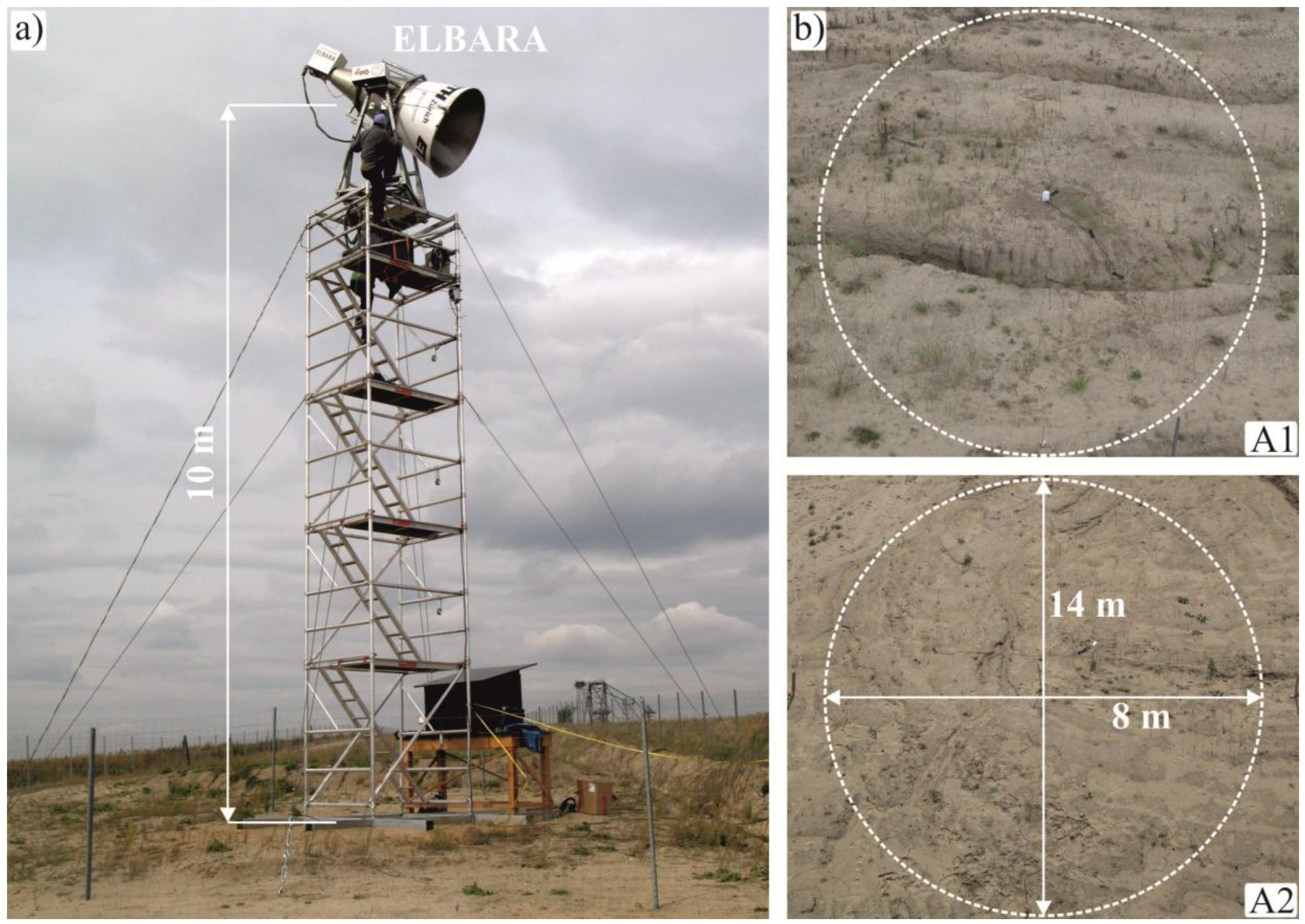
2.1. Investigation Area and General Setup

In the late summer of 2008, the ETH L-BAnd RAdiometer (ELBARA) [26] was installed in the artificial research catchment “Chicken Creek” [27,28], close to the city of Cottbus in Eastern Germany (51°36′N, 14°16′E; 130 m a.s.l.). This catchment area was established as a joint research site of the interdisciplinary research project “Structures and Processes of the Initial Ecosystem Development Phase in an Artificial Water Catchment” [29]. It was completed in 2005 and then left to allow an ecosystem to develop without further restrictions and with minimum interference. Shortly after its completion, distinct erosion gullies had begun to develop in the catchment area. They developed rapidly at first, but once the gully network had formed, they remained fairly stable over time. Due to these distinct erosion gullies in combination with the comprehensive monitoring network present, the catchment was considered to be well suited to investigate relief effects on L-band emission under natural, but well-characterized, conditions.

ELBARA was mounted on a tower at the southwestern boundary of the research catchment with the phase center of the receiving horn antenna approximately 10 m above the ground (Figure 1). The radiometer was equipped with an automated elevation stage [30], making it possible to change its view direction in elevation to perform regular sky measurements for calibration purposes. Furthermore, a revolving platform [31] enabled to change the radiometer’s view direction also in azimuth, and therewith to measure brightness temperatures of two footprints with different surface characteristics quasi-simultaneously.

Figure 1. (a) ELBARA, mounted on the tower and looking toward footprint A1 at the observation angle θ_RM = 55°. (b) The investigated areas A1 and A2. The dashed circles show approximately the −12 dB footprint areas and the arrows indicate their dimensions. The footprint ellipses appear as circles since the pictures were taken oblique to the surface from the top of the radiometer tower.

Figure 1. (a) ELBARA, mounted on the tower and looking toward footprint A1 at the observation angle θ_RM = 55°. (b) The investigated areas A1 and A2. The dashed circles show approximately the −12 dB footprint areas and the arrows indicate their dimensions. The footprint ellipses appear as circles since the pictures were taken oblique to the surface from the top of the radiometer tower.

Footprint Area 1 (A1, situated within the research catchment) was crossed by two very distinct parallel erosion gullies (≈0.5 m deep) with steep and differently oriented slopes. A third less distinct gully ran through A1 approximately midway between the other two. Footprint Area 2 (A2), situated just outside the catchment, was leveled and smoothed prior to beginning the measurements to restore the area to a state comparable to the initial state of the research catchment just after completion. No distinct gullies were therefore present in A2 at the start of the measurement campaign, and the surface can be regarded as smooth. Both areas were covered with only very sparse vegetation (A1) or none at all (A2), and its presence is assumed to have no significant influence on the L-band brightness temperatures measured. The soil material of both areas is a sandy substrate several meters thick, underlain by a layer of clay. The substrate is characterized as loamy sand with a bulk density of approximately 1700 kg∙m⁻³ and a porosity between 31% and 38% [27]. Neither the relief nor the vegetation cover in A1 changed significantly throughout the measurement campaign. In A2, a sparse vegetation cover similar to that in A1 developed in 2009, while the relief remained approximately the same during the campaign.

2.2. Brightness-Temperature Measurements

Brightness temperatures were measured with the ETH L-BAnd RAdiometer (ELBARA) [26]. This Dicke-type radiometer is equipped with a dual-mode Picket-horn antenna [32] with 23.5 dB gain and a −3 dB full beam width of ±6° around the antenna main direction. ELBARA measures brightness temperatures $T_{\text{B}}^p$ at horizontal (p = H) and vertical (p = V) polarization in the protected frequency range 1400–1427 MHz, corresponding to a vacuum wavelength of λ ≈ 0.21 m. All measurements are recorded with 12 s integration time, resulting in an absolute accuracy of the measured $T_{\text{B}}^p$ of around ±1 K and a sensitivity better than 0.1 K. Instrumental noise was estimated by comparing measured sky brightness temperatures with theoretical L-band sky brightness and corrected for in the $T_{\text{B}}^p$ measured according to [33].

Quasi-simultaneous $T_{\text{B}}^p$ measurements of the footprints A1 and A2 (Figure 1b) were carried out from October 2008 until the end of 2009. One complete measuring cycle consisted of 22 individual $T_{\text{B}}^p$ measurements. First, 16 measurements of A1 were carried out, before ELBARA rotated toward A2. Then, six $T_{\text{B}}^p$ measurements of A2 were taken, before ELBARA rotated back toward A1, and the measuring cycle started again. The individual $T_{\text{B}}^p$ measurements were initiated every five minutes, and a whole measuring cycle lasted 120 min. Both footprints were observed at the fixed radiometer observation angle θ_RM = 55° relative to the vertical direction. Sky measurements for external calibration were performed on a regular basis about once every month at θ_RM = 140°. Due to several failures of the power supply and a broken gear belt connecting the motor with the revolving stage, the time series of $T_{\text{B}}^p$ contains several gaps and after August 2009 only measurements of A1 are available. Nevertheless, measurements could be made during all seasons and from mid-February until mid-May 2009 an almost uninterrupted time series of $T_{\text{B}}^p$ measurements of both scenes was obtained.

2.3. Hydrometeorological and in situ Soil Measurements

Hydrometeorological measurements were carried out in the established monitoring network [34]. Meteorological variables (precipitation, air temperature, relative humidity, shortwave radiation and wind speed) were recorded by two standard weather stations every 10 min, and daily webcam images provided estimates of snow cover and snow depth. Groundwater level measurements were made manually at least once a month in groundwater observation pipes located on a 20 m × 20 m grid across the catchment. Volumetric soil-water content and soil temperature were recorded at numerous locations both inside and outside the gullies in the catchment area, and also specifically in the two footprints observed by the radiometer. We used ECH₂O EC-TM sensors from Decagon Devices [35], which were installed upright at 10–15 cm depth. For the sake of clarity it is mentioned here that these in situ measurements are used to calibrate the soil-water and heat-transfer model to estimate high resolution (2 mm) soil moisture and temperature profiles, ultimately used to simulate soil emissivities as will be described in Section 3.1.

2.4. Topography Measurements

To analyze the impact of surface relief on the $T_{\text{B}}^p$ measured, we relied on accurate Digital Terrain Models (DTM) of the two footprints A1 and A2. These were derived from terrestrial laser scanning, carried out with the time-of-flight laser scanner RIEGL LMS-Z420i [36] in August 2009. The scanner was mounted on the highest platform of the radiometer tower (≈3 m beneath the pivotal point of ELBARA), and had approximately the same view of the footprints as the radiometer. Additionally, two scans were made with the scanner set up on a mobile tower and looking toward ELBARA, to obtain information about the gully slopes facing away from the radiometer.

After a first post-processing of the raw scan data with the RiSCAN PRO 1.4.3 software package [36] (merging of the measurements from the radiometer tower with the measurements from the mobile tower, clipping of the data to the observed scenes, removal of measurement points related to vegetation), the resulting surface patches of both areas were converted to ESRI raster data sets for further manipulation in ArcGIS [37]. Above all, the irregularly spaced scan data were interpolated to a regular 5 cm × 5 cm grid using surface analysis tools of Arc-GIS (ESRI 2011. ArcGIS Desktop: Release 10. Environmental Systems Research Institute: Redlands, CA, USA), yielding the DTMs of the footprints A1 and A2. These DTMs consist of the spatial coordinates X = (x, y, z) of every grid cell, which describe the elevation z of 5 cm × 5 cm facets at position (x, y). Furthermore, the unit vectors $\widehat{n}=\nabla \cdot X/\left|X\right|$, normal to the facets’ surfaces, were calculated as the gradients ($\nabla =\left(\partial /\partial x,\partial /\partial y,\partial /\partial z\right)$) of the facet position vectors X using Arc-GIS. Facets that cannot be seen from the radiometer were identified and flagged as invisible. Finally, the facets of footprint A1 situated inside the erosion gullies were flagged as such, in order to discriminate between areas inside and outside the erosion gullies in the brightness-temperature simulations (Section 3).

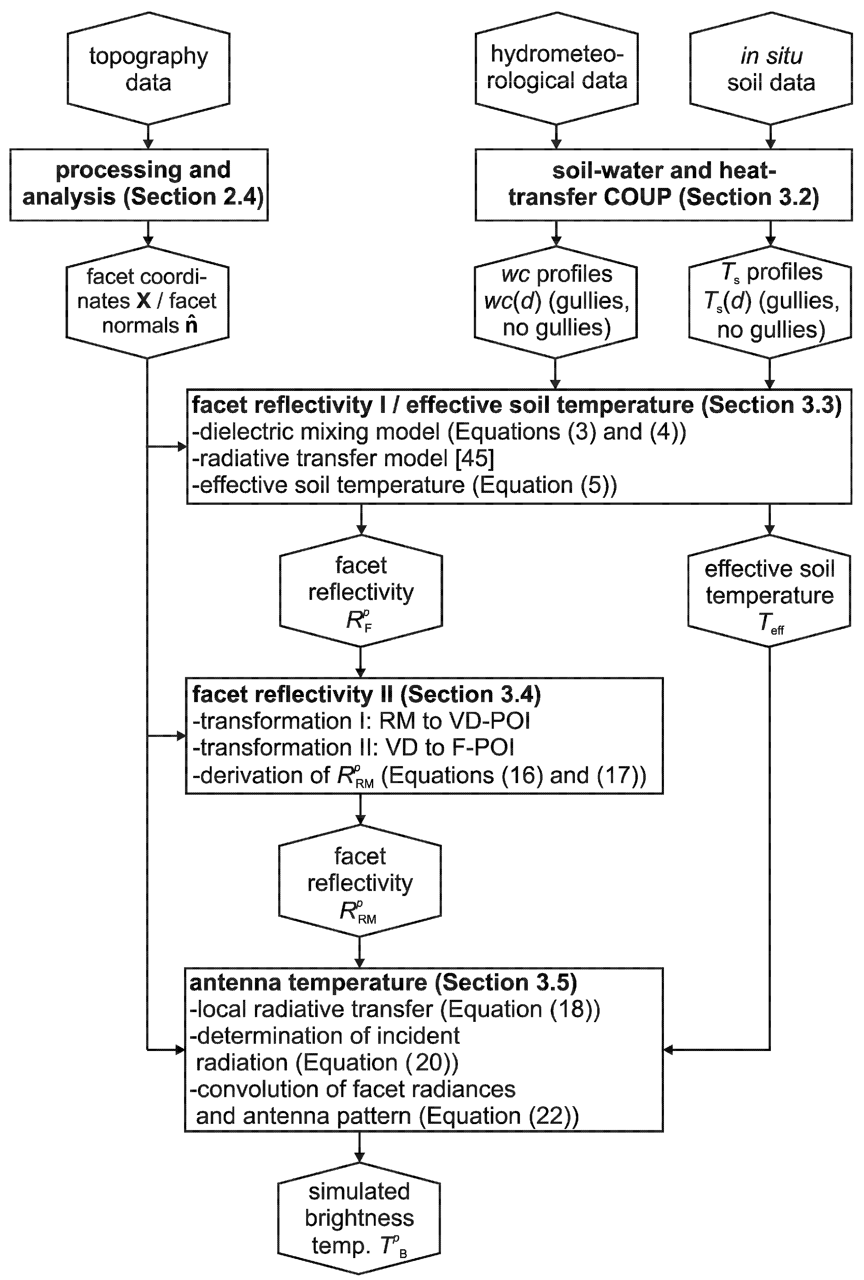
3. Brightness-Temperature Simulations

The radiance received by a microwave radiometer observing a land surface is composed of surface and atmospheric contributions, both of which depend, amongst other things, on the relief [38]. This relief-dependency is explicitly included in our emission model in order to relate differences observed between the emissions $T_{\text{B}}^p$ from footprints A1 and A2 to corresponding differences in their surface relief. That means the different local observation angles and orientations of the plane of linear polarization of different regions within the radiometer footprints are considered. Furthermore, the shadowing of some regions from the downwelling sky radiance by the surrounding elevated terrain is taken into account.

To this end, a facet model was implemented. The actual footprint surfaces were approximated by mosaics of small planar surface elements (facets), corresponding to the 5 cm × 5 cm pixels of the DTMs, which are tangent to the local surface. The locations of the individual facets are given by their spatial coordinates X, and the facets’ inclination (tilt) and orientation (aspect) are described by the associated surface normals $\widehat{n}$. The facets were assumed to be locally smooth and specularly reflecting. For assigning soil temperature and water content we discriminated between facets inside and outside the erosion gullies. Otherwise, soil temperature and water content were assumed as uniform within both footprint areas. In a first step, the radiative contribution of each individual facet to the emission of the full scene toward the radiometer is calculated. Subsequently, the total scene emission received by the radiometer was modeled as the convolution of the local facet emissions and the antenna’s directional sensitivity. Similar facet models were proposed, e.g., in [18,39], and have been used, e.g., to describe the microwave emission of a mountainous region in Northern Italy in [22], although for facet dimensions much larger than the observation wavelength. However, using facets with dimensions 5 cm × 5 cm smaller than the observation wavelength λ ≈ 21 cm, as we do in this study, is still appropriate since spatial gradients of facet emissions are in most cases very small, implying that local surfaces can be well approximated by tangent planes of dimensions of the observation wavelength (λ ≈ 21 cm). Accordingly, the incoherent superposition of electric fields emitted from 5 cm × 5 cm facets yields very much the same result as if electric fields emitted from 20 cm × 20 cm facet were summed up coherently. This was tested by evaluating our emission model for facets with dimensions 20 cm × 20 cm comparable with the observation wavelength (λ ≈ 21 cm), which were derived from the 5 cm × 5 cm facets by spatial smoothing (a 4 × 4 pixel window was applied). This exercise yielded almost unchanged results for the simulated total scene emission compared to using 5 cm × 5 cm facets. Beyond this model-based argumentation, the suitability of using facets with dimensions of 5 cm < λ ≈ 21 cm is also confirmed experimentally in [40], where microwave measurements at 2–12 GHz were successfully reproduced by a model also assuming incoherent superposition of radiances emitted from facets that are smaller than the observation wavelength.

3.1. General Modeling Approach

When calculating the emission from an individual facet toward the RadioMeter (RM), located at X_RM = (x_RM, y_RM, z_RM), one has to consider the tilt angle and orientation (aspect) of the facet as well as the deviation of the antenna main axis k_RM from the view direction k_F = X_RM − X from the Facet (F) toward the radiometer (Figure 2). For this reason, we introduce three Planes Of Incidence (POI) and corresponding elevation angles, as depicted in Figure 2.

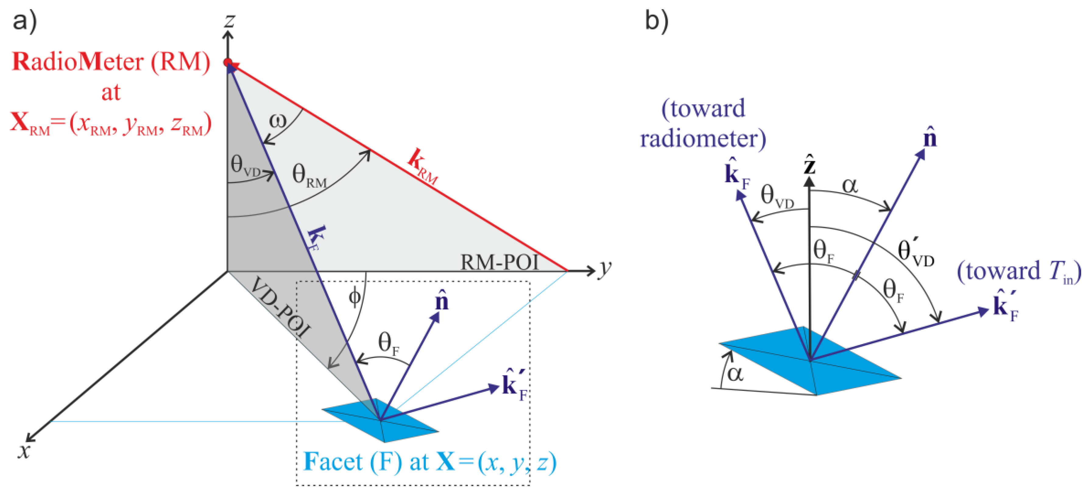
• The RadioMeter Plane Of Incidence (RM-POI) is normal to the xy-plane, and comprises the antenna main axis k_RM. Hence, it is spanned by the two unit vectors ${\widehat{k}}_{\text{RM}}=k_{\text{RM}}/\left|k_{\text{RM}}\right|$ and the vertical ẑ = (0, 0, 1). The corresponding radiometer elevation angle θ_RM = 55° is the nadir angle of the antenna main axis.
• The View-Direction Plane Of Incidence (VD-POI) of a Facet (F) is also normal to the xy-plane, but is spanned by the two unit vectors ${\widehat{k}}_{\text{F}}=k_{\text{F}}/\left|k_{\text{F}}\right|$ and ẑ, and is thus rotated in azimuth by the angle ϕ with respect to the RM-POI. The corresponding view-direction elevation angle θ_VD is the angle at which a facet is seen from the radiometer, and is given by the scalar product:

  $$\cos {\theta }_{\text{VD}}=\widehat{z}\cdot {\widehat{k}}_{\text{F}}$$

  (1)
• The local or Facet Plane Of Incidence (F-POI) is normal to the facet’s surface and is spanned by ${\widehat{k}}_{\text{F}}$ and the facet’s surface normal $\widehat{n}$. The corresponding facet elevation angle θ_F is the incidence angle of radiation incident on a facet that is reflected in the specular direction toward the radiometer. It is given by:

  $$\cos {\theta }_{\text{F}}=\widehat{n}\cdot {\widehat{k}}_{\text{F}}$$

  (2)

  and thus deviates from θ_VD for facet tilt angles α ≠ 0°.

Figure 2. (a) Illustration of the setup considered when calculating the reflection on and emission from a tilted facet. The RadioMeter (RM) is mounted at X_RM = (x_RM, y_RM, z_RM) with the observation angle θ_RM = 55° relative to the vertical, and the antenna main axis k_RM. The Facet (F) is at X = (x, y, z) and tilted with respect to the horizontal by the angle α. It is observed from the radiometer at the View-Direction (VD) elevation angle θ_VD, and k_F is the view direction from the facet to the radiometer. The facet’s surface normal is $\widehat{n}$ and θ_F is the facet elevation angle. The vector ${\widehat{k}}_{\text{F}}^{\prime }$ points toward the radiation T_in incident on the facet that is reflected toward the radiometer. Additionally, the angle ω between k_RM and k_F and the azimuth angle ϕ between the RM-POI and the VD-POI (grey-shaded areas) are shown. (b) Cut-out of the dotted box in (a) illustrating the relationship between the unit vectors ${\widehat{k}}_{\text{F}}$, ${\widehat{k}}_{\text{F}}^{\prime }$, ẑ, $\widehat{n}$ and the angles $\alpha$, ${\theta }_{\text{F}}$, ${\theta }_{\text{VD}}$, ${\theta }_{\text{VD}}^{\prime }$. The F-POI (not especially illustrated for the sake of better readability) comprises the vectors $\widehat{n}$, ${\widehat{k}}_{\text{F}}$ and ${\widehat{k}}_{\text{F}}^{\prime }$, but not necessarily the vertical ẑ.

Figure 2. (a) Illustration of the setup considered when calculating the reflection on and emission from a tilted facet. The RadioMeter (RM) is mounted at X_RM = (x_RM, y_RM, z_RM) with the observation angle θ_RM = 55° relative to the vertical, and the antenna main axis k_RM. The Facet (F) is at X = (x, y, z) and tilted with respect to the horizontal by the angle α. It is observed from the radiometer at the View-Direction (VD) elevation angle θ_VD, and k_F is the view direction from the facet to the radiometer. The facet’s surface normal is $\widehat{n}$ and θ_F is the facet elevation angle. The vector ${\widehat{k}}_{\text{F}}^{\prime }$ points toward the radiation T_in incident on the facet that is reflected toward the radiometer. Additionally, the angle ω between k_RM and k_F and the azimuth angle ϕ between the RM-POI and the VD-POI (grey-shaded areas) are shown. (b) Cut-out of the dotted box in (a) illustrating the relationship between the unit vectors ${\widehat{k}}_{\text{F}}$, ${\widehat{k}}_{\text{F}}^{\prime }$, ẑ, $\widehat{n}$ and the angles $\alpha$, ${\theta }_{\text{F}}$, ${\theta }_{\text{VD}}$, ${\theta }_{\text{VD}}^{\prime }$. The F-POI (not especially illustrated for the sake of better readability) comprises the vectors $\widehat{n}$, ${\widehat{k}}_{\text{F}}$ and ${\widehat{k}}_{\text{F}}^{\prime }$, but not necessarily the vertical ẑ.

With the different planes of incidence and corresponding elevation angles defined, we followed the course of action illustrated in Figure 3 to simulate the $T_{\text{B}}^p$ of the footprints A1 and A2. First, we calculated volumetric soil-water content and soil-temperature profiles for areas inside and outside gullies for the entire time span of the experiment with a numerical soil-water and heat-transfer model (Section 3.2). The soil-water content profiles were converted into soil-permittivity profiles and subsequently used as input to a coherent radiative transfer model for layered dielectric media. Evaluating this model yielded the facet reflectivities $R_{\text{F}}^p$ (θ_F) at polarization p = H, V with respect to the F-POI and at the elevation angle θ_F at the respective times of the radiometer measurements. Furthermore, also the effective soil temperatures T_eff(θ_F) were computed from the soil-temperature and soil-permittivity profiles (Section 3.3). In the next step, we performed a transformation from the F-POI to the RM-POI to derive the facets’ reflectivities $R_{\text{RM}}^p$ at polarization p = H, V with respect to the RM-POI (Section 3.4). This transformation accounts for the deviation of the facets’ view directions ${\widehat{k}}_{\text{F}}$ from the antenna main axis ${\widehat{k}}_{\text{RM}}$ as well as for the rotation of the direction of linear polarization resulting from the tilt of the facets.

The facet reflectivities $R_{\text{RM}}^p$ were then used in a simple radiative transfer model to calculate the radiances of the individual facets toward the radiometer. In doing so, shadowing effects caused by the relief were taken into account. The individual radiative contributions of all facets within the respective footprint were then summed up to provide the total simulated antenna temperatures for the two footprints, taking into account the antenna’s directivity as well as projection effects (Section 3.5). This yielded simulated brightness temperatures $T_{\text{B}}^p$ for the footprints A1 and A2 at all times of radiometer measurements to be directly compared to the measured time series of brightness temperatures of the two footprints.

Figure 3. Flowchart of the modeling chain followed to simulate brightness temperatures. Hexagons indicate model in- and outputs. Boxes show the different model components, which are explained in the sections indicated by the numbers in parentheses.

Figure 3. Flowchart of the modeling chain followed to simulate brightness temperatures. Hexagons indicate model in- and outputs. Boxes show the different model components, which are explained in the sections indicated by the numbers in parentheses.

3.2. Soil-Water Content and Soil-Temperature Profiles

The volumetric soil-water content wc(d) and soil-temperature T_s(d) (d = depth below surface) profiles were simulated at one-hour time intervals using the one-dimensional numerical soil-water and heat-transfer model COUP [14,41]. The model calculates the water and heat fluxes from the soil surface to a depth of 3 m for a layered vertical soil profile with predefined thermal and hydrological properties. The upper boundary conditions of the profile are governed by the soil-surface energy balance, which takes into account the evaporation fluxes and a potentially present snow cover. To this end, hourly measurements of precipitation, air temperature, relative humidity, shortwave radiation, and wind speed were used as the driving model variables. Furthermore, the monthly groundwater-level measurements were averaged across the investigated area, interpolated in time, and then used as the lower hydraulic boundary condition for the simulations. The vertical water flow in the unsaturated zone was calculated with the Richards equation [42], using water-retention curves (i.e., the relationship between soil suction and water content) parameterized according to Brooks and Corey [43] and the Mualem function [44] for unsaturated hydraulic conductivity. The applied parameter values (Table 1) were based on site-specific information on soil texture and in situ hydraulic conductivity measurements [27], and further tuned to give a best match with the in situ wc and T_s measurements at a depth of 10–15 cm.

Table 1. Soil parameter values used in the soil-water and heat-transfer model (COUP) for the simulation of the soil-water content and soil-temperature profiles (wc_sat = saturation water content, Ψ_a = air entry pressure, λ_p = pore size distribution index, wc_res = residual water content, k_sat^a and k_sat^b = saturated hydraulic conductivity including and excluding macropores).

Soil Depth (m)	wcsat(m3∙m−3)	Ψa (cm)	λp (−)	wcres (m3∙m−3)	ksata (mm∙d−1)	ksatb (mm∙d−1)
0–0.06	0.27	15	0.60	0.055	200	50
0.06–0.30	0.31	15	0.60	0.055	2500	250
0.30–0.70	0.28	10	0.15	0.080	4000	400
0.70–3.00	0.26	10	0.15	0.082	3000	300

Table 1. Soil parameter values used in the soil-water and heat-transfer model (COUP) for the simulation of the soil-water content and soil-temperature profiles (wc_sat = saturation water content, Ψ_a = air entry pressure, λ_p = pore size distribution index, wc_res = residual water content, k_sat^a and k_sat^b = saturated hydraulic conductivity including and excluding macropores).

Soil Depth (m)	wcsat(m3∙m−3)	Ψa (cm)	λp (−)	wcres (m3∙m−3)	ksata (mm∙d−1)	ksatb (mm∙d−1)
0–0.06	0.27	15	0.60	0.055	200	50
0.06–0.30	0.31	15	0.60	0.055	2500	250
0.30–0.70	0.28	10	0.15	0.080	4000	400
0.70–3.00	0.26	10	0.15	0.082	3000	300

The COUP model was first run to derive wc(d) and T_s(d) profiles for a typical location outside the erosion gullies. In a second model run, corresponding profiles for a typical gully were simulated by considering a ≈50 cm shorter distance to the groundwater table (as opposed to the first model run applied to locations outside erosion gullies), and thus a higher and more uniform water content close to the soil surface. The physical soil properties were assumed to be the same inside and outside gullies. The simulated wc(d) and T_s(d) profiles were subsequently used as inputs to the radiative transfer model applied to compute the facet reflectivities $R_{\text{F}}^p$ at local incidence angles θ_F as well as for the determination of the effective soil temperature T_eff (Section 3.3).

3.3. Facet Reflectivities with Respect to the F-POI and Effective Soil Temperatures

The facet reflectivities $R_{\text{F}}^p$ (θ_F) at polarization p = H, V with respect to the F-POI and at the elevation angle θ_F were computed with a coherent radiative transfer model for layered dielectric media [45]. The model is based on a matrix formulation of the boundary conditions at the layer interfaces derived from Maxwell’s Equations. Inputs to the model are the soil-permittivity profile ε(d), observation wavelength λ, polarization p, and the facet elevation angle θ_F. The model was evaluated for dielectric layers with a thickness of 2 mm << λ = 21 cm, and the total thickness of the dielectric stack corresponded with the profile depth of 3 m available from the COUP simulations.

The complex permittivity profiles ε(d) = ε′(d) + i ·ε″(d) were generated from the wc(d) profiles calculated by the COUP model (Section 3.2) as follows. First, simulated wc were linearly interpolated to the depths of the layers considered in the radiative transfer model (the soil depths indicated in Table 1 interpolated to 2 mm). Then, real parts ε′(d) were derived from wc(d) using the empirical mixing model [46], applicable to mineral soils with 0 m³∙m⁻³ ≤ wc ≤ 0.55 m³∙m⁻³:

$${\epsilon }^{\prime }\left(d\right)=3.03+9.3wc\left(d\right)+146.0w{c}^2\left(d\right)-76.7w{c}^3\left(d\right)$$

(3)

This purely empirical mixing model, doing without any additional soil-specific information, was chosen, as the soil material in the investigation area is a sandy substrate [27] rather than a naturally developed, undisturbed soil (Section 2.1). Imaginary parts ε″(d) were estimated as:

$${\epsilon }^{″}\left(d\right)={\epsilon }_{\text{w}}^{″}\cdot wc\left(d\right)$$

(4)

where ε_w″ is the imaginary part of the permittivity of water. To simulate ε_w″ at λ = 21 cm and soil temperature T_s, we used the model [47] and considered the soil’s salinity to be S = 5 ppt (parts per thousand by weight), which is a reasonable value for soil water [48].

The radiative transfer model [45] was evaluated for all dielectric profiles ε(d) derived from the simulated wc(d) profiles, yielding time series of facet reflectivities $R_{\text{F}}^p$ (θ_F) for locations inside and outside the erosion gullies at hourly intervals. Since the radiometer measurements were carried out at shorter intervals (≈5 min), we subsequently interpolated these values to the times of the radiometer measurements to derive the $R_{\text{F}}^p$ (θ_F) for all times when radiometer measurements were available.

Effective soil temperatures T_eff(θ_F), determining upwelling brightness temperatures emitted from the soil, were subsequently computed from the soil profiles ε(d) and T_s(d) using the approach described in, e.g., [49]:

$$\begin{array}{ll}{T}_{\text{eff}}\left({\theta }_{\text{F}}\right)={\displaystyle {\int }_0^{\infty }{T}_{\text{s}}\left(d\right)\cdot \frac{\gamma \left(d\right)}{\cos \theta \left(d\right)}\cdot \exp \left[-\tau \left(d\right)\right]\cdot dd}\hfill & \text{with}\hfill \\ \theta \left(d\right)=\arcsin \left(\frac{\sin {\theta }_{\text{F}}}{\mathrm{Re}\left(\sqrt{\epsilon \left(d\right)}\right)}\right);\gamma \left(d\right)=\frac{4\pi }{\lambda }\cdot \mathrm{Im}\left(\sqrt{\epsilon \left(d\right)}\right);\hfill & \tau \left(d\right)={\displaystyle {\int }_0^d\frac{\gamma \left(d^{\prime }\right)}{\cos \theta \left(d^{\prime }\right)}\cdot d{d}^{\prime }}\hfill \end{array}$$

(5)

where γ(d) is the depth profile of power absorption coefficients that result from dielectric losses in the soil, τ(d) is the associated optical-thickness profile, and θ(d) are the propagation angles in the soil at depth d. Using Equation (5), effective temperatures T_eff(θ_F) were computed for locations inside and outside erosion gullies, and subsequently also interpolated to the times of the radiometer measurements.

3.4. Facet Reflectivities with Respect to the RM-POI

The facet reflectivities $R_{\text{RM}}^p$ at polarization p = H, V and at the local incidence angle with respect to the RM-POI (Figure 2) were derived from the previously calculated $R_{\text{F}}^p$ (θF). To this end and in accordance with Kirchhoff’s law (e.g., [50]), we reversed the field propagation directions and considered the radiometer to be a “transmitter” of p-polarized radiation with the unit field vector ${\widehat{E}}_{\text{RM}}^p$ with $\left|{\widehat{E}}_{\text{RM}}^p\right|=1$. Of course, the reciprocity of Maxwell’s equations is the fundamental physical justification permitting the reversal of the field propagation directions. Furthermore, the sky was regarded as a “receiver” absorbing the total energy carried by the field E_ref reflected along the forward direction on the facet. This implies that $R_{\text{RM}}^p$ is the ratio between the reflected energy carried by E_ref and the incident energy transmitted by the radiometer. As the energy carried by an electric field is proportional to its squared field amplitude, the reflectivity $R_{\text{RM}}^p$ is defined as:

$$R_{\text{RM}}^p\equiv \frac{{\left|E_{\text{ref}}\right|}^2}{{\left|{\widehat{E}}_{\text{RM}}^p\right|}^2}$$

(6)

To determine |E_ref| = E_ref, the transmitted field ${\widehat{E}}_{\text{RM}}^p$ was first decomposed into its horizontal and vertical components ${\mathbf{E}}_{\text{F}}^{\text{H}}$ and ${\mathbf{E}}_{\text{F}}^{\text{V}}$ with respect to the F-POI, which are reflected on the facet with the reflectivities $R_{\text{F}}^{\text{H}}$ (θ_F) and $R_{\text{F}}^{\text{V}}$ (θ_F), respectively. This means, once the fields ${\mathbf{E}}_{\text{F}}^p$ incident on the facet are known, the reflectivities $R_{\text{F}}^p$ (θ_F) computed beforehand (Section 3.3) can be used to calculate E_ref and, in turn, $R_{\text{RM}}^p$ using Equation (6). Determining ${\mathbf{E}}_{\text{F}}^P$ from ${\widehat{E}}_{\text{RM}}^p$ requires the following steps: (1) Calculation of the field ${\widehat{E}}_{\text{RM}}^p$ transmitted by the radiometer at the location of each individual facet within the footprints, as the antenna main axis $-{\widehat{k}}_{\text{RM}}$ deviates from the antenna’s view direction $-{\widehat{k}}_{\text{F}}$ toward the facet (Figure 2); and (2) determining the components ${\mathbf{E}}_{\text{F}}^{\text{H}}$ and ${\mathbf{E}}_{\text{F}}^{\text{V}}$ from ${\widehat{E}}_{\text{RM}}^p$, which are p-polarized with respect to the F-POI.

3.4.1. Transformation I: RM-POI to VD-POI

To determine the polarization unit vectors ${\widehat{E}}_{\text{RM}}^p$ (p = H, V) for each individual facet, we use the Ludwig-2 definition [51], stating that the two cross polarization directions are tangent to a spherical surface. Figuratively speaking, this corresponds to considering the radiometer to be the sum of many infinitesimal radiometers looking towards each individual facet along $-{\widehat{k}}_{\text{F}}$. The direction of H-polarization for each infinitesimal radiometer is normal to both ${\widehat{k}}_{\text{F}}$ and the vertical $\widehat{z}$, and thus parallel to $\widehat{z}\times {\widehat{k}}_{\text{F}}$. Consequently, ${\widehat{E}}_{\text{RM}}^{\text{H}}$ is given by:

$${\widehat{E}}_{\text{RM}}^{\text{H}}=\frac{\widehat{z}\times {\widehat{k}}_{\text{F}}}{\left|\widehat{z}\times {\widehat{k}}_{\text{F}}\right|}$$

(7)

Similarly, ${\widehat{E}}_{\text{RM}}^{\text{V}}$ is determined from ${\widehat{E}}_{\text{RM}}^{\text{H}}$ and ${\widehat{k}}_{\text{F}}$ as:

$${\widehat{E}}_{\text{RM}}^{\text{V}}=\frac{{\widehat{E}}_{\text{RM}}^{\text{H}}\times {\widehat{k}}_{\text{F}}}{\left|{\widehat{E}}_{\text{RM}}^{\text{H}}\times {\widehat{k}}_{\text{F}}\right|}$$

(8)

3.4.2. Transformation II: VD-POI to F-POI

The electric field ${\widehat{E}}_{\text{RM}}^p$ incident on a tilted facet is p-polarized with respect to the VD-POI, but not with respect to the facet’s surface (Figure 2). It is rotated by an angle φ with respect to the facet surface in a plane perpendicular to the incidence direction, because the facet’s surface normal $\widehat{n}$ deviates from the vertical $\widehat{z}$. To derive the locally, i.e., with respect to the F-POI p’-polarized components ${\mathbf{E}}_{\text{F}}^{p{p}^{’}}$ from ${\widehat{E}}_{\text{RM}}^p$, we projected ${\widehat{E}}_{\text{RM}}^p$ onto the polarization directions p’ = H, V with respect to the F-POI, given by the two unit vectors:

$$\begin{array}{ll}{\widehat{E}}_{\text{F}}^{\text{H}}=\frac{\widehat{n}\times {\widehat{k}}_{\text{F}}}{\left|\widehat{n}\times {\widehat{k}}_{\text{F}}\right|}\hfill & \text{for }{p}^{\prime }=\text{H, and}\hfill \\ {\widehat{E}}_{\text{F}}^{\text{V}}=\frac{{\widehat{E}}_{\text{F}}^{\text{H}}\times {\widehat{k}}_{\text{F}}}{\left|{\widehat{E}}_{\text{F}}^{\text{H}}\times {\widehat{k}}_{\text{F}}\right|}\hfill & \text{for }{p}^{\prime }=\text{V}\hfill \end{array}$$

(9)

Projecting ${\widehat{E}}_{\text{RM}}^{\text{H}}$ onto the two directions given by Equation (9) yields the two field vectors:

$$\begin{array}{l}{E}_{\text{F}}^{\text{HH}}=\left({\widehat{E}}_{\text{RM}}^{\text{H}}\cdot {\widehat{E}}_{\text{F}}^{\text{H}}\right){\widehat{E}}_{\text{F}}^{\text{H}}\\ E_{\text{F}}^{\text{HV}}=\left({\widehat{E}}_{\text{RM}}^{\text{H}}\cdot {\widehat{E}}_{\text{F}}^{\text{V}}\right){\widehat{E}}_{\text{F}}^{\text{V}}\end{array}$$

(10)

and proceeding equally for ${\widehat{E}}_{\text{RM}}^{\text{V}}$ yields:

$$\begin{array}{l}{E}_{\text{F}}^{\text{VH}}=\left({\widehat{E}}_{\text{RM}}^{\text{V}}\cdot {\widehat{E}}_{\text{F}}^{\text{H}}\right){\widehat{E}}_{\text{F}}^{\text{H}}\\ E_{\text{F}}^{\text{VV}}=\left({\widehat{E}}_{\text{RM}}^{\text{V}}\cdot {\widehat{E}}_{\text{F}}^{\text{V}}\right){\widehat{E}}_{\text{F}}^{\text{V}}\end{array}$$

(11)

The angle φ of polarization rotation is the angle between ${\widehat{E}}_{\text{RM}}^{\text{H}}$ and ${\widehat{E}}_{\text{F}}^{\text{H}}$, and is determined from their scalar product:

$$\cos \phi ={\widehat{E}}_{\text{RM}}^{\text{H}}\cdot {\widehat{E}}_{\text{F}}^{\text{H}}$$

(12)

3.4.3. Derivation of $R_{\text{RM}}^p$

Using the calculations described above, we now determine $R_{\text{RM}}^p$ in the RM-POI as follows: The electric field ${\widehat{E}}_{\text{RM}}^{\text{H}}$ transmitted by the radiometer and incident on a facet is expressed by means of the two orthogonal fields ${\mathbf{E}}_{\text{F}}^{\text{HH}}$ and ${\mathbf{E}}_{\text{F}}^{\text{HV}}$ (Equation (10)), which are H- and V-polarized, respectively, with respect to the F-POI:

$${\widehat{E}}_{\text{RM}}^{\text{H}}=E_{\text{F}}^{\text{HH}}+E_{\text{F}}^{\text{HV}}$$

(13)

The energies propagated by these fields are reflected on the facet with $R_{\text{F}}^{\text{H}}$ and $R_{\text{F}}^{\text{V}}$, respectively, yielding the following expression for the magnitudes of the reflected fields:

$${\left|E_{\text{F, ref}}^{p{p}^{\prime }}\right|}^2=R_{\text{F}}^{p^{\prime }}{\left|E_{\text{F}}^{p{p}^{\prime }}\right|}^2$$

(14)

The total field E_ref reflected on the facet (as used in Equation (6)) is the linear combination of all the reflected fields ${\mathbf{E}}_{\text{F,ref}}^{p{p}^{’}}$. Thus using Equation (14), we can write for the magnitude E_ref = |E_ref|:

$${\left({\text{E}}_{\text{ref}}\right)}^2={\left|E_{\text{ref}}\right|}^2=R_{\text{F}}^{\text{H}}{\left|E_{\text{F}}^{\text{HH}}\right|}^2+R_{\text{F}}^{\text{V}}{\left|E_{\text{F}}^{\text{HV}}\right|}^2$$

(15)

Inserting Equation (15) into Equation (6) and substituting $\left|{\widehat{E}}_{\text{RM}}^{\text{H}}\right|=1$, we eventually get:

$$R_{\text{RM}}^{\text{H}}=R_{\text{F}}^{\text{H}}{\left|E_{\text{F}}^{\text{HH}}\right|}^2+R_{\text{F}}^{\text{V}}{\left|E_{\text{F}}^{\text{HV}}\right|}^2$$

(16)

for the facet reflectivity $R_{\text{RM}}^{\text{H}}$ at horizontal polarization with respect to the RM-POI.

Following the corresponding procedure for a transmitted field ${\widehat{E}}_{\text{RM}}^{\text{V}}$ and thereby using Equation (11) to derive the field components ${\mathbf{E}}_{\text{F}}^{p{p}^{’}}$ yields:

$$R_{\text{RM}}^{\text{V}}=R_{\text{F}}^{\text{H}}{\left|E_{\text{F}}^{\text{VH}}\right|}^2+R_{\text{F}}^{\text{V}}{\left|E_{\text{F}}^{\text{VV}}\right|}^2$$

(17)

for the facet reflectivity $R_{\text{RM}}^{\text{V}}$ at vertical polarization with respect to the RM-POI.

3.5. Antenna Brightness Temperature

Knowing the facet reflectivities $R_{\text{RM}}^p$ at polarization p = H, V and at the local incidence angle with respect to the RM-POI, the brightness temperature radiated by each individual facet in direction ${\widehat{k}}_{\text{F}}$ toward the radiometer was calculated with:

$$T_{\text{B},f}^p=\left(1-R_{\text{RM}}^p\right)T_{\text{eff}}+R_{\text{RM}}^p{T}_{\text{in}}$$

(18)

This simple radiative transfer model fulfills Kirchhoff’s law, and describes the p-polarized brightness temperature $T_{\text{B},f}^p$ radiated from a facet with reflectivity $R_{\text{RM}}^p$ and effective physical temperature T_eff as the sum of the radiation emitted from the facet and the fraction of radiation T_in incident on the facet that is reflected toward the radiometer. For facets illuminated by the sky, the radiation T_in is the sky radiation T_sky, which is computed as the sum of downwelling atmosphere emission and cosmic background attenuated by the atmosphere, which depend on air temperature profile, elevation above sea level and angle of incidence according to the statistical parameterization given in the Appendix of [52]. For facets, which are obscured from the sky by their surroundings, T_in is set to T_in = T_eff, implying that the surroundings are considered as black-body radiator at effective physical temperature T_eff.

To assign T_in, we first determined the direction ${\widehat{k}}_{\text{F}}^{\prime }=\left(2\cos {\theta }_{\text{F}}\cdot \widehat{n}\right)-{\widehat{k}}_{\text{F}}$ toward T_in, which follows from the relationship ${\widehat{k}}_{\text{F}}+{\widehat{k}}_{\text{F}}^{\prime }=\cos {\theta }_{\text{F}}\left|{\widehat{k}}_{\text{F}}\right|\widehat{n}+\cos {\theta }_{\text{F}}\left|{\widehat{k}}_{\text{F}}^{\prime }\right|\widehat{n}$ between ${\widehat{k}}_{\text{F}}$, ${\widehat{k}}_{\text{F}}^{\prime }$ and $\widehat{n}$ (Figure 2b). Then, we computed the polar angle ${\theta }_{\text{VD}}^{\prime }$ between the vertical $\widehat{z}$ and ${\widehat{k^{\prime }}}_{\text{F}}$ from the scalar product:

$$\cos {\theta }_{\text{VD}}^{\prime }={\widehat{k}}_{\text{F}}^{\prime }\cdot \widehat{z}$$

(19)

and assuming a flat horizon (i.e., facets with ${\theta }_{\text{VD}}^{\prime }\le 90°$ are illuminated by the sky, whereas facets with ${\theta }_{\text{VD}}^{\prime }>90°$ are obscured from the sky by their surroundings) we assigned:

$$T_{\text{in}}=\{\begin{array}{cc}{T}_{\text{sky}}\hfill & \text{for facets with }{\theta }_{\text{VD}}^{\prime }\le 90°\hfill \\ T_{\text{eff}}\hfill & \text{for facets with }{\theta }_{\text{VD}}^{\prime }>90°\hfill \end{array}$$

(20)

On the one hand, this simple criterion is, in the vast majority, valid to distinguish between facets illuminated by the sky or by surrounding facets. On the other hand it is simple enough to avoid excessive computational demand, which would result when applying e.g., a ray-tracing approach.

With $R_{\text{RM}}^p$, T_eff, and T_in known for each individual facet, we calculated the contributions $T_{\text{B},f}^p$ of all visible facets within a footprint (f = 1,…,n, where n denotes the total number of all facets visible from the radiometer) to the total radiance received by the radiometer by Equation (18). Subsequently, these contributions $T_{\text{B},f}^p$ were summed up to the total radiance $T_{\text{B}}^p$ received by the radiometer antenna, taking into account the antenna’s directivity D(ω) as well as the fact that the facets appear enlarged or reduced in size, depending on their elevation angle θ_F and slope α (projection effect). The directivity D(ω) of ELBARA’s horn antenna can be approximated by D(ω) = exp(−0.01781 ω²) [33], where ω is the polar angle (in units of degrees) between the antenna main axis k_RM and the view direction of a facet k_F. The projection effect is taken into account by means of the solid angle Ω at which a facet appears as seen from the antenna position X_RM:

$$\mathrm{\Omega }=A\cdot \frac{\cos {\theta }_{\text{F}}}{r^2}=\frac{A^{\text{h}}}{\cos \alpha }\cdot \frac{\cos {\theta }_{\text{F}}}{r^2}$$

(21)

where A is the true area of the facet, A^h = (5 × 5) cm² is the projection of A onto a horizontal plane, and r is the distance between the facet and the antenna. The slope α of the facet is the same as the tilt angle between its surface normal $\widehat{n}$ and the vertical $\widehat{z}$ and is calculated from the scalar product as $\cos \alpha =\widehat{z}\cdot \widehat{n}$. Finally, the total radiance $T_{\text{B}}^p$ received by the radiometer antenna was calculated as the beam-weighted sum of the radiances $T_{\text{B},f}^p$ from all visible facets f = 1,…,n within the footprint area:

$$T_{\text{B}}^p=\frac{{\displaystyle \sum _{f=1}^n{D}_f{T}_{\text{B},f}^p{\mathrm{\Omega }}_f}}{{\displaystyle \sum _{f=1}^n{D}_f{\mathrm{\Omega }}_f}}$$

(22)

4. Results

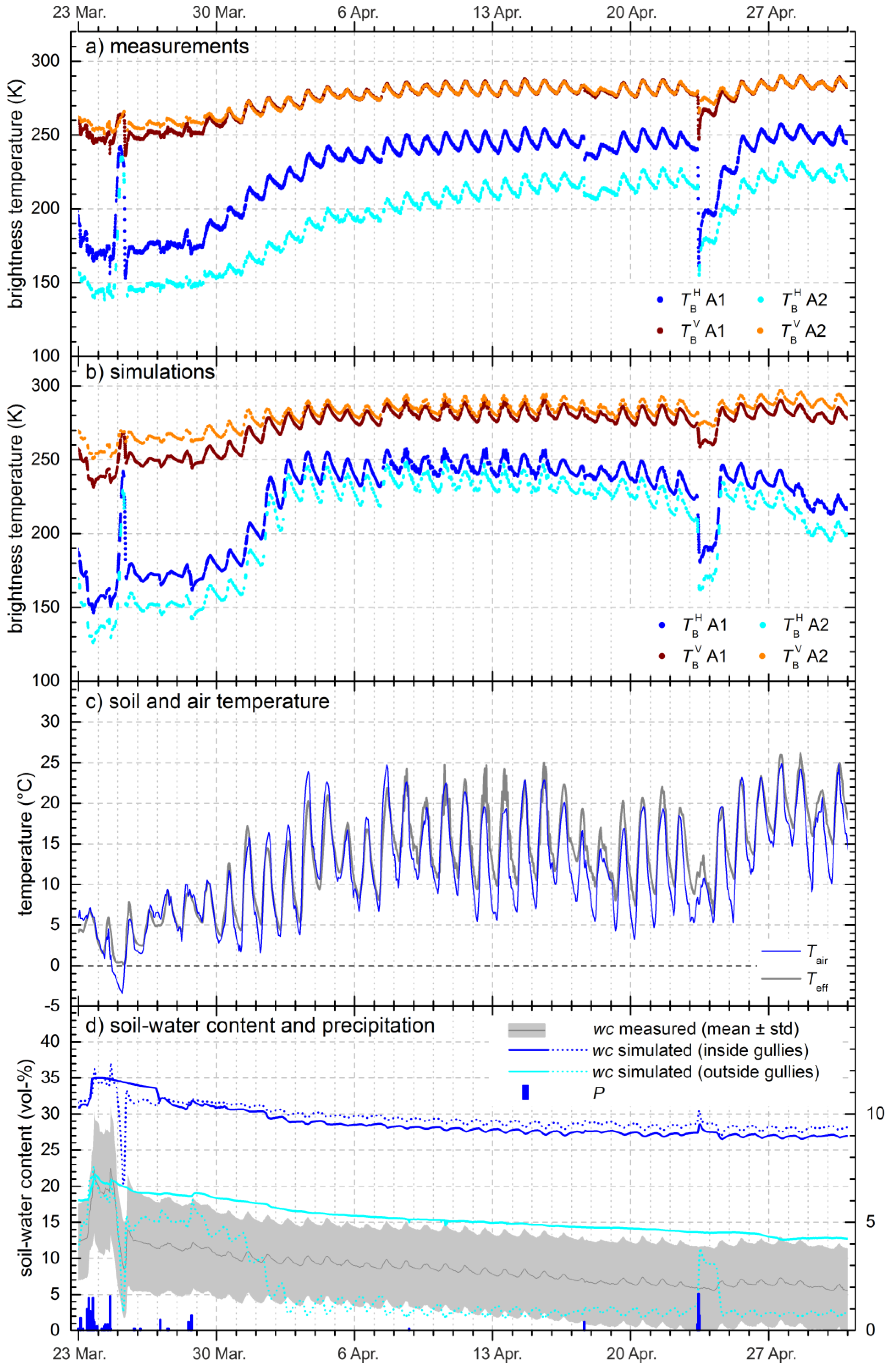
4.1. Meteorological Conditions

During the measurement campaign from October 2008 to December 2009, the meteorological station in the research catchment recorded 778 mm of precipitation, which is close to the long-term average [27]. Several intense rainfall events occurred in autumn 2008, with the most intense rainfall on 29 and 30 October (40 mm in two days), while spring 2009 was very dry. During April and the first half of May, hardly any precipitation at all was recorded. The most intense rainfall events in summer 2009 were 20 mm on 1 July and 17 mm on 4 July, both lasting less than one hour. Early autumn 2009 was again drier than in typical years.

Both winters (2008/2009 and 2009/2010) were colder than average. The soil was snow-covered for approximately half of the time from mid-November 2008 to the end of February 2009. On some days, however, only the gullies were filled with snow, while the other areas were mostly snow-free. During the first half of January and the second half of February 2009, when most snow (5–10 cm) was observed, the footprint areas were entirely snow-covered, with large spatial differences in snow depth due to wind drift. In winter 2009/2010, an intermittent snow cover was observed after 12 December.

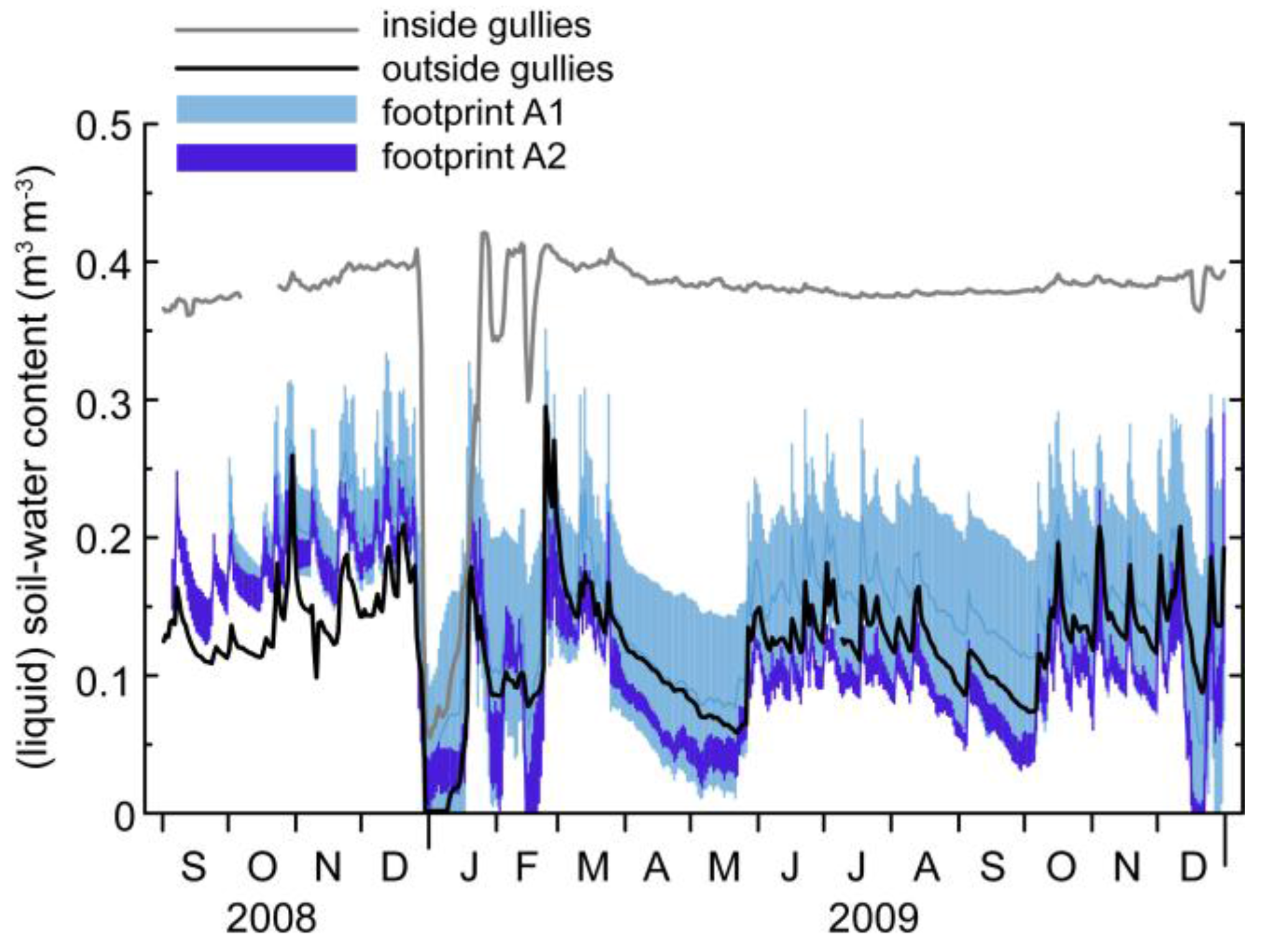
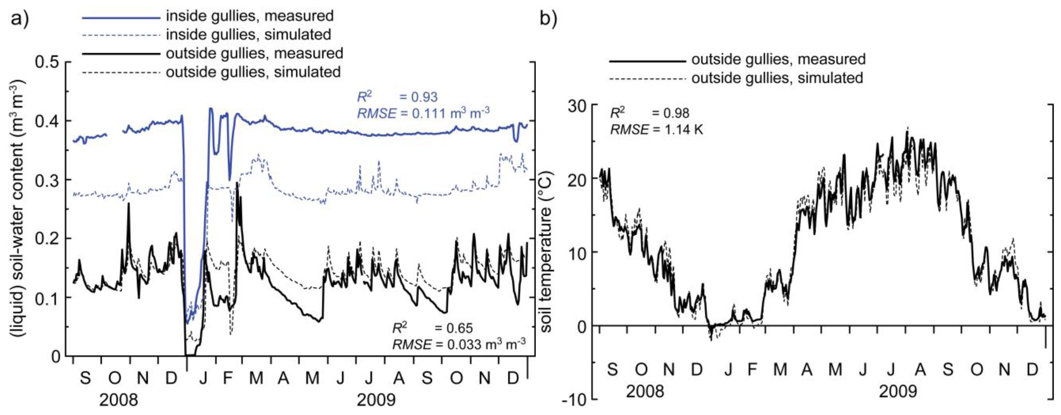
4.2. Measured and Simulated Soil-Water Content and Soil-Temperature Dynamics

The in situ measurements of the liquid soil-water content wc were distinctly different for locations inside and outside the erosion gullies (Figure 4). Inside the gullies (grey line), wc was generally higher, with little temporal change except for January and February 2009 when the soil was freezing. Outside the gullies (black line), wc showed much more short-term dynamics, clearly responding to individual events, such as rainfall and snowmelt as well as the freezing/thawing and drying of the soil.

Figure 4. Liquid soil-water content wc measured at a depth of 10–15 cm. The grey line represents the mean wc of the five sensors distributed inside of erosion gullies within the footprint area A1 shown in Figure 1. The black line shows the mean wc of the 15 sensors installed outside of erosion gullies within the areas A1 and A2. Light blue and dark blue areas indicate the mean wc ± standard deviation of the five measurements each, carried out specifically within footprint A1 (representing areas both inside and outside gullies) and within footprint A2 (no gullies present), respectively. The very low values in January, February and December 2009 are due to soil freezing.

Figure 4. Liquid soil-water content wc measured at a depth of 10–15 cm. The grey line represents the mean wc of the five sensors distributed inside of erosion gullies within the footprint area A1 shown in Figure 1. The black line shows the mean wc of the 15 sensors installed outside of erosion gullies within the areas A1 and A2. Light blue and dark blue areas indicate the mean wc ± standard deviation of the five measurements each, carried out specifically within footprint A1 (representing areas both inside and outside gullies) and within footprint A2 (no gullies present), respectively. The very low values in January, February and December 2009 are due to soil freezing.

The wc measurements within the leveled footprint A2 (dark blue area) showed a rather narrow range of spatial variation and were similar to the measurements outside the erosion gullies elsewhere in the catchment. In contrast, the five sensors in the footprint A1 with the gullies detected much more spatial variation since they represent areas both inside and outside the gullies (light blue area). The presence of gullies in A1 led also to a higher mean wc in A1 than in A2.

After the calibration of the COUP model (Section 3.2), wc simulated for areas outside the gullies correlated well with the corresponding measurements (Figure 5a, black lines). Overall, an R²-value of 0.65 and a root-mean-square error (RMSE) of 0.03 m³∙m^–3 attest a good model performance for these areas. The temporal variation of wc inside the gullies was somewhat overestimated by the model, whereas the absolute values were underestimated by approximately 0.1 m³∙m^–3 for almost the entire measurement campaign (blue lines). Soil temperatures T_s at the depth 10–15 cm were reproduced very well by the COUP simulations (Figure 5b), suggesting that the surface energy balance and the vertical heat flux in the soil (which depends on wc, amongst other things) are appropriately simulated. The difference in T_s for areas inside and outside the gullies was very small and the correspondence between the simulations and the measurements was similar for both (R² = 0.98, RMSE = 1.14 K).

The satisfactory agreement of simulations and in situ measurements for the 10–15 cm soil layer suggests that these model results are a reasonable choice as input to the reflectivity and local radiative transfer model applied (Section 3.3 and Section 3.5) to simulate brightness temperatures in a forward approach for comparison with the radiometer measurements.

Figure 5. (a) Measured and simulated time series of liquid soil-water content wc at a depth of 10–15 cm. For the measurements, the mean wc of 15 sensors located outside the gullies (solid black line) and the mean wc of five sensors representing typical gully locations (solid blue line) are displayed. (b) Corresponding time series of soil temperatures T_s for areas outside the gullies. Soil temperatures T_s inside the gullies were very similar and are not shown for the sake of clarity.

Figure 5. (a) Measured and simulated time series of liquid soil-water content wc at a depth of 10–15 cm. For the measurements, the mean wc of 15 sensors located outside the gullies (solid black line) and the mean wc of five sensors representing typical gully locations (solid blue line) are displayed. (b) Corresponding time series of soil temperatures T_s for areas outside the gullies. Soil temperatures T_s inside the gullies were very similar and are not shown for the sake of clarity.

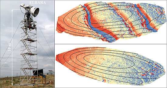
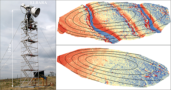
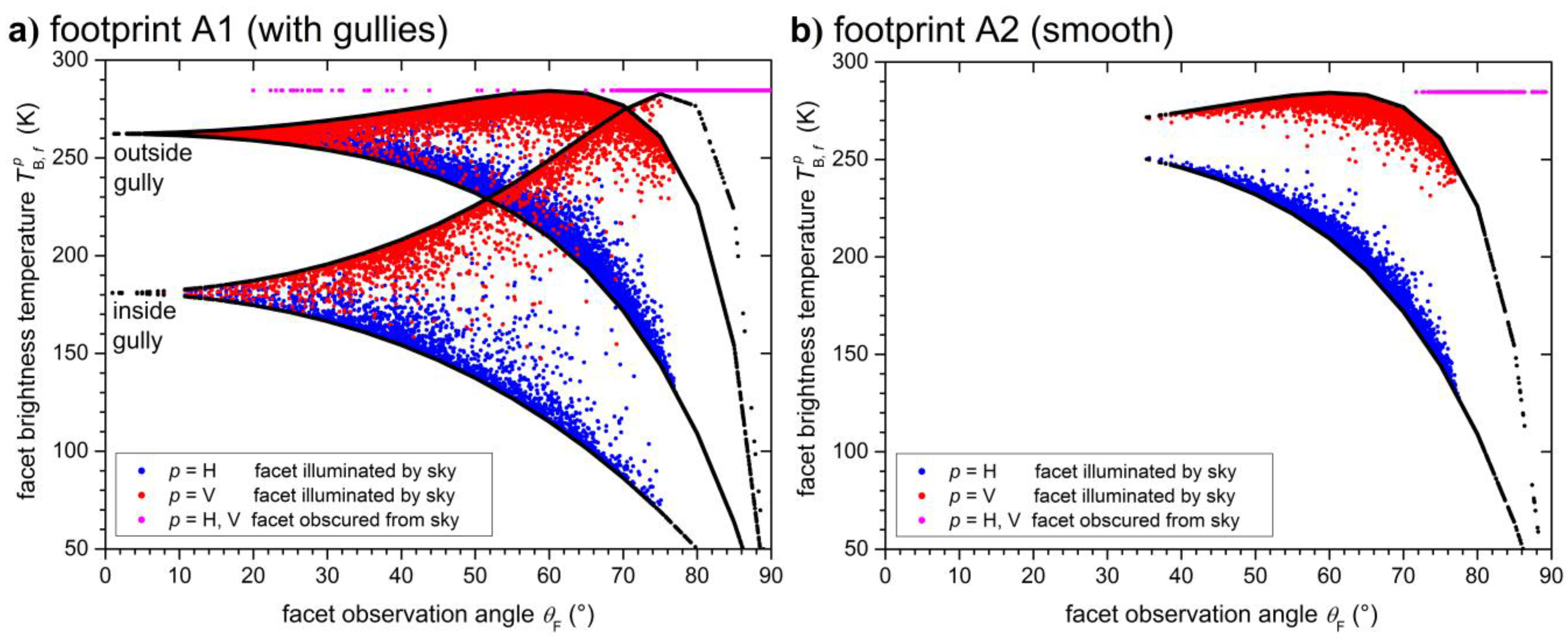
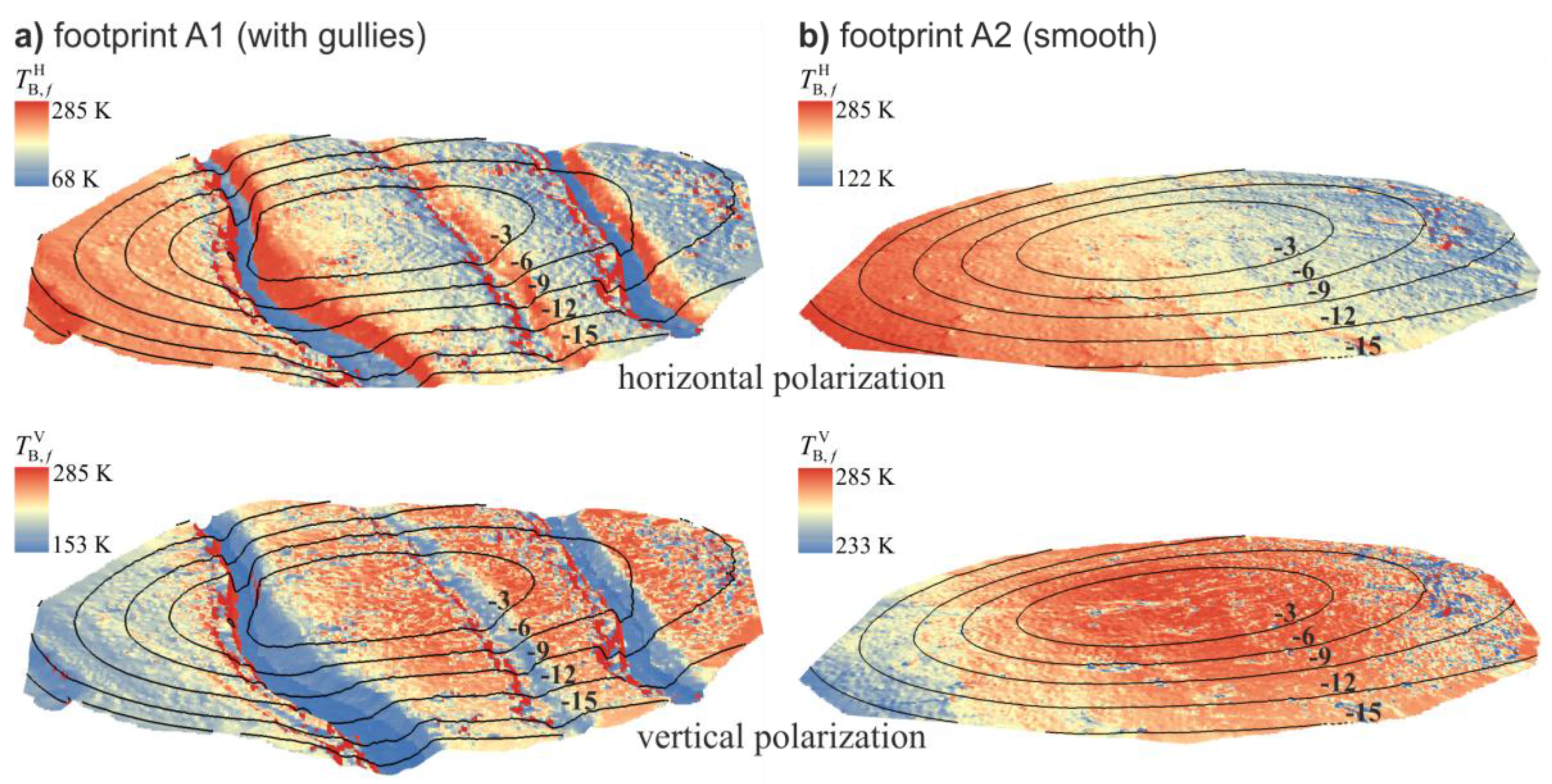
4.3. Footprint Topographies and Exemplary Brightness-Temperature Simulation

Table 2 gives a summary of the geometrical parameters (defined in Figure 2) relevant for the emission of the observed footprints. These parameters were derived from the DTMs of the footprints A1 (with gullies) and A2 (smooth surface) and the viewing configuration of the radiometer. The angles ϕ, ω, and θ_VD represent the deviation of the VD-POI from the RM-POI of the different facets within A1 and A2. Since the DTMs cover about the same fraction of both footprint areas, the ranges of ϕ, ω, and θ_VD are approximately the same for both. The angles α, θ_F, and φ, on the other hand, illustrate above all the different surface characteristics (relief) of both footprints. Due to the steep slopes of the gullies in A1 the ranges of tilt angles α and, consequently, also of facet elevation angles θ_F are much wider in A1 than in A2. Low values of θ_F in A1 are mostly associated with facets in gully slopes facing the radiometer, whereas facets in slopes facing away from the radiometer usually exhibit values θ_F > 90°. The range of θ_F encountered in the smooth footprint A2, however, mainly resembles differences caused by the different locations of the facets within the footprint area. This is in accordance with the fact that, in A2, the range of θ_F is not much wider than the range of θ_VD, whereas in A1 the difference between both is substantial. Correspondingly, the angle of polarization rotation φ spans the whole range between 0° and 90° in A1, but is always smaller than 40° in A2.

Due to the gullies in A1, about 6% of the facets (mainly situated in gully slopes facing away from the radiometer) were invisible for ELBARA, whereas in A2 almost all facets were visible. Furthermore, the range of elevation angles θ′_VD of the radiation incident on the facets is much wider in A1 than in A2, and much more facets are obscured from the sky and illuminated by the surrounding landscape in A1 (≈7%) than in A2 (<1%).

Table 2. Geometrical parameters (symbols are defined in Figure 2) determining the relief-dependent emission behavior of the footprints A1 and A2. Numbers in parentheses show the respective values just for the facets visible for ELBARA.

Parameter	Footprint A1	Footprint A2
total number n of facets/area of footprint	48,529/121 m2	60,089/150 m2
number of invisible facets	3077	99
number of facets in gullies	3666 (2546)	0
number of facets receiving radiation from the surrounding landscape	3466 (1619)	445 (380)
distance r between radiometer and facets	13.18 m ≤ r ≤ 25.26 m	14.22 m ≤ r ≤ 29.64 m
azimuth angle ϕ between ${\widehat{k}}_{\text{RM}}$ and ${\widehat{k}}_{\text{F}}$	0° ≤ ϕ ≤ 23°	0° ≤ ϕ ≤ 21°
polar angle ω between ${\widehat{k}}_{\text{RM}}$ and ${\widehat{k}}_{\text{F}}$	0° ≤ ω ≤ 19°	0° ≤ ω ≤ 18°
view-direction elevation angle θVD	36° ≤ θVD ≤ 66°	39° ≤ θVD ≤ 66°
slope (tilt angle) α	0° ≤ α ≤ 75°	0° ≤ α ≤ 43°
facet elevation angle θF	1° ≤ θF ≤ 127°	35° ≤ θF ≤ 97°
angle φ of polarization rotation	0° ≤ φ ≤ 90°	0° ≤ φ ≤ 40°
elevation angle θ’VD of radiation incident on the facets	1° ≤ θ’VD ≤ 179°	14° ≤ θ’VD ≤ 129°

Table 2. Geometrical parameters (symbols are defined in Figure 2) determining the relief-dependent emission behavior of the footprints A1 and A2. Numbers in parentheses show the respective values just for the facets visible for ELBARA.

Parameter	Footprint A1	Footprint A2
total number n of facets/area of footprint	48,529/121 m2	60,089/150 m2
number of invisible facets	3077	99
number of facets in gullies	3666 (2546)	0
number of facets receiving radiation from the surrounding landscape	3466 (1619)	445 (380)
distance r between radiometer and facets	13.18 m ≤ r ≤ 25.26 m	14.22 m ≤ r ≤ 29.64 m
azimuth angle ϕ between ${\widehat{k}}_{\text{RM}}$ and ${\widehat{k}}_{\text{F}}$	0° ≤ ϕ ≤ 23°	0° ≤ ϕ ≤ 21°
polar angle ω between ${\widehat{k}}_{\text{RM}}$ and ${\widehat{k}}_{\text{F}}$	0° ≤ ω ≤ 19°	0° ≤ ω ≤ 18°
view-direction elevation angle θVD	36° ≤ θVD ≤ 66°	39° ≤ θVD ≤ 66°
slope (tilt angle) α	0° ≤ α ≤ 75°	0° ≤ α ≤ 43°
facet elevation angle θF	1° ≤ θF ≤ 127°	35° ≤ θF ≤ 97°
angle φ of polarization rotation	0° ≤ φ ≤ 90°	0° ≤ φ ≤ 40°
elevation angle θ’VD of radiation incident on the facets	1° ≤ θ’VD ≤ 179°	14° ≤ θ’VD ≤ 129°

To show the influence of surface relief on L-band emission, on the one hand, and to illustrate the modeling chain described in Section 3, on the other, we show the detailed results of a brightness-temperature simulation for one single time step in Figure 6 and Figure 7. The effective soil temperature T_eff = 11.4 °C was approximately the same everywhere in A1 and A2 at that time, whereas the soil-moisture difference for areas inside (wc = 0.27 m³∙m⁻³) and outside the gullies (wc = 0.14 m³∙m⁻³) was at a maximum. The simulated brightness temperatures were $T_{\text{B}}^{\text{H}}$ = 224.8 K and $T_{\text{B}}^{\text{V}}$ = 274.6 K for footprint A1 and $T_{\text{B}}^{\text{H}}$ = 210.0 K and $T_{\text{B}}^{\text{V}}$ = 281.9 K for footprint A2.

Figure 6 shows the facet brightness temperatures $T_{\text{B},f}^p$ at p = H, V of all facets f = 1, …, n in A1 and A2 computed with Equation (18). To this end, the wc(d) profiles simulated with the COUP model (Section 3.2) and the facet elevation angles θ_F derived from the DTMs of the footprint surfaces (Section 2.4) were used in the coherent radiative transfer model (Section 3.3) to compute the facet reflectivities $R_{\text{F}}^p$ (θ_F) with respect to the F-POI. Subsequently, the facet reflectivities $R_{\text{RM}}^p$ with respect to the RM-POI needed in Equation (18) were derived from $R_{\text{F}}^p$ by considering the rotation of the direction of linear polarization for the tilted facets (Section 3.4.1 and Section 3.4.2). Furthermore, the criterion Equation (20) was used to determine the radiation T_in that is incident on the facets and reflected towards the radiometer. Blue and red dots show the resulting $T_{\text{B},f}^p$ of facets illuminated by the sky. They are in the range 66.5 K ≤ $T_{\text{B},f}^{\text{H}}$ ≤ 277.6 K and 147.3 K ≤ $T_{\text{B},f}^{\text{V}}$ ≤ 284.2 K for A1, and 125.8 K ≤ $T_{\text{B},f}^{\text{H}}$ ≤ 251.5 K and 231.5 K ≤ $T_{\text{B},f}^{\text{V}}$ ≤ 284.2 K for A2. The magenta dots denote the $T_{\text{B},f}^p$ of facets obscured from the sky and receiving radiation from the surrounding landscape at the effective temperature T_eff = 284.5 K.

Figure 6. Brightness temperatures $T_{\text{B},f}^p$ (p = H, V) of all facets in footprint (a) A1 and (b) A2 calculated with the facet model for 23 April 2009, 9:12 a.m. Blue and red dots are $T_{\text{B},f}^p$ at horizontal and vertical polarization, respectively, of facets illuminated by the sky. Magenta dots show $T_{\text{B},f}^p$ at both polarizations of facets obscured from sky radiance, and thus receiving radiation from the surrounding landscape. To demonstrate the impact of polarization mixing and shadowing on facet emission, additionally facet $T_{\text{B},f}^p$ are shown, which were calculated neglecting these effects (black dots).

Figure 6. Brightness temperatures $T_{\text{B},f}^p$ (p = H, V) of all facets in footprint (a) A1 and (b) A2 calculated with the facet model for 23 April 2009, 9:12 a.m. Blue and red dots are $T_{\text{B},f}^p$ at horizontal and vertical polarization, respectively, of facets illuminated by the sky. Magenta dots show $T_{\text{B},f}^p$ at both polarizations of facets obscured from sky radiance, and thus receiving radiation from the surrounding landscape. To demonstrate the impact of polarization mixing and shadowing on facet emission, additionally facet $T_{\text{B},f}^p$ are shown, which were calculated neglecting these effects (black dots).

Figure 7. Facet brightness temperatures $T_{\text{B},f}^p$ from Figure 6 overlain on the DTMs of footprint (a) A1 and (b) A2 at p = H (top) and p = V (bottom). The DTMs are shown so that the view direction toward ELBARA (situated to the left and above) is approximately the same for both. The isolines show the directivity D(ω) of the ELBARA antenna in dB projected onto the DTMs.

Figure 7. Facet brightness temperatures $T_{\text{B},f}^p$ from Figure 6 overlain on the DTMs of footprint (a) A1 and (b) A2 at p = H (top) and p = V (bottom). The DTMs are shown so that the view direction toward ELBARA (situated to the left and above) is approximately the same for both. The isolines show the directivity D(ω) of the ELBARA antenna in dB projected onto the DTMs.

To demonstrate the impact of polarization mixing and shadowing on facet emission, additionally $T_{\text{B},f}^p$ are shown, where only the different observation angles θ_F of the facets were considered in the calculations (black dots). To this end, the reflectivity term $R_{\text{RM}}^p$ in Equation (18) was replaced with the facet reflectivities $R_{\text{F}}^p$ (θ_F) and all facets were assigned T_in = T_sky regardless of whether they are illuminated by the sky or not. The comparison with the previously calculated values illustrates the distinct influence of polarization mixing (resulting from the rotation of the direction of linear polarization) on facet emission. Values, obtained with polarization mixing included in the calculations, are significantly increased at p = H (blue dots) and decreased at p = V (red dots) compared to the values calculated neglecting this effect (black dots). Moreover, it can be seen that the impact of polarization mixing is more pronounced in footprint A1 with the distinct relief. Furthermore, considerably more facets in A1 receive radiation from the surrounding landscape than in footprint A2, where the surface is smooth.

In Figure 7, the facet radiances $T_{\text{B},f}^p$ shown in Figure 6 are overlain on the DTMs of A1 and A2 to give an impression of the dependence of the $T_{\text{B},f}^p$ on the facets’ locations within the footprint, on the one hand, and the tilt of the facets, on the other. In both footprints, we see a decrease (p = H) or increase (p = V) in $T_{\text{B},f}^p$ in the direction away from ELBARA (toward the right) for facets situated outside the erosion gullies. This change in the $T_{\text{B},f}^p$ corresponds to the differing elevation angles θ_F of these facets, which range roughly from 40° (left) to 70° (right). At vertical polarization, $T_{\text{B},f}^{\text{V}}$ actually start to decrease again for large θ_F exceeding the Brewster angle at approximately 65°, which can be observed to some extent in the illustration for p = V (bottom).

At the bottom of the gullies in A1, $T_{\text{B},f}^p$ are colder than in the surroundings at both polarizations, as a result of the generally higher wc within the gullies. The elevation angles θ_F of the gully slopes facing the radiometer (toward left) are approximately in the range 10° ≤ θ_F ≤ 30°, resulting in rather high (p = H) and low (p = V) values, respectively, for the $T_{\text{B},f}^p$ of these slopes. For most of the slopes facing away from the radiometer (toward the right), θ_F is larger than 60°. This leads to significantly colder $T_{\text{B},f}^{\text{H}}$ and slightly warmer $T_{\text{B},f}^{\text{V}}$ than in the surroundings. Due to their steepness, however, most of these slopes receive radiation from the surrounding landscape and display therefore the highest $T_{\text{B},f}^p$ within both areas.

4.4. Brightness-Temperature Time Series

Figure 8 shows the measurement and simulation results for the time period from 23 March to 1 May 2009. Several distinctive weather conditions occurred in this representative period, making it well suited to investigate process-driven brightness-temperature variations and their dependence on the footprints’ surface characteristics for a wide range of environmental conditions. The first two days of the selected time period were rainy and cold, and were then followed by a brief frost event with soil freezing. Afterwards, there was no significant precipitation for four weeks and it gradually became warmer, resulting in an extended drying period for the soil. This dry spell was interrupted by two rainfall events, which differed in duration as well as in the amount of precipitation. At the end of the period shown, dry and warm conditions prevailed again (the complete time series of measurement and simulation results from October 2008 until the end of 2009 are provided as Supplementary Material, pp. 2–9)

4.4.1. Measurements

In general, brightness temperature $T_{\text{B}}^p$ (p = H, V) measured (Figure 8a) clearly reflect the weather and soil conditions prevailing at the time. First of all, $T_{\text{B}}^p$ follow the dynamics of the effective soil temperature T_eff, which in turn is correlated with the air temperature T_air (Figure 8c). This is most obvious in the diurnal $T_{\text{B}}^p$ variations, corresponding to the diurnal cycle of temperature and solar irradiation. Superimposed on this underlying trend are more rapid changes in $T_{\text{B}}^p$ due to short-term changes in ambient conditions (e.g., the onset of precipitation or soil frost) and rather long-term trends in $T_{\text{B}}^p$ due to more gradual changes, such as soil drying.

Precipitation leads to an increase in soil-water content wc shortly after the onset of precipitation (Figure 8d), which, in turn, results in decreasing $T_{\text{B}}^p$ . This can be observed, e.g., on 23/24 March. The moderate but steady rainfall (11 mm in two days), accompanied by low air and soil temperatures, resulted in an increase in measured wc and a decrease in $T_{\text{B}}^p$ . At both polarizations, this $T_{\text{B}}^p$ decrease was more pronounced in footprint A1, featuring the distinct relief in the form of erosion gullies, than in the smooth footprint A2.

After precipitation stops, $T_{\text{B}}^p$ usually start to increase again with decreasing wc. In the example period shown, this effect was even further enhanced by soil freezing. Soil freezing leads to a sudden loss of liquid wc, as most water in the soil-pore spaces freezes, which, in turn, lowers soil permittivity significantly and hence increases the microwave emission [14,53,54]. During the brief soil-frost event shown in Figure 8, T_air dropped below 0 °C and T_eff reached the freezing point in the night of 24 to 25 March. This resulted in a pronounced decrease in the wc measured as well as an abrupt increase in $T_{\text{B}}^p$.

Shortly after, the soil thawed again leading to a renewed wc increase and a sudden drop in $T_{\text{B}}^p$ . Corresponding sharp spikes are visible in the $T_{\text{B}}^p$ of both footprints. At p = V, these changes were more pronounced in A1, whereas at p = H the changes in $T_{\text{B}}^{\text{H}}$ associated with soil freezing and thawing were somewhat more pronounced in A2.

In prolonged periods of prevailing warm and dry conditions $T_{\text{B}}^p$ gradually increase as the soil’s temperature rises and the soil dries out, whereas the rate of this $T_{\text{B}}^p$ increase often differs for both footprints. For example, during the almost three-week long dry spell starting on 29 March, the initial increase in $T_{\text{B}}^{\text{V}}$ at p = V was somewhat greater in A1 than in A2, so that the $T_{\text{B}}^{\text{V}}$ of both areas approached each other and were then almost identical for several weeks. At p = H, the initial increase in $T_{\text{B}}^{\text{H}}$ was more pronounced in A1 as well. After 8 April, however, the $T_{\text{B}}^{\text{H}}$ of A1 remained approximately stationary, whereas the $T_{\text{B}}^{\text{H}}$ of A2 was still increasing.

In addition, the following decrease in $T_{\text{B}}^p$ associated with the small rainfall event on 17 April was more pronounced in A1 than in A2 at both polarizations, and the same general behavior was observed after the more intense rainfall on 23 April, whereas the associated $T_{\text{B}}^p$ decrease was much larger. Quite peculiar to note in this context is that neither the very small rainfall on 17 April (0.4 mm in 1 h) nor the larger rainfall on 23 April (3 mm in 2 h) are visible in the wc measured, but nevertheless led to noticeable drops in $T_{\text{B}}^p$ (except for $T_{\text{B}}^{\text{V}}$ in A2 on 17 April).

Figure 8. Measured and simulated $T_{\text{B}}^p$ for the observation angle θ_RM = 55° for 23 March to 1 May 2009. (a) Measured $T_{\text{B}}^p$ (p = H, V) of footprints A1 (with gullies) and A2 (smooth); (b) corresponding $T_{\text{B}}^p$ simulated for A1 and A2; (c) air temperature T_air and effective soil temperature T_eff; and (d) lines indicate liquid soil-water content wc simulated for areas inside and outside erosion gullies for the 0–3 cm (dotted lines) and 10–15 cm (solid lines) soil layer. The grey-shaded area is the range mean ± standard deviation of the ten in situ wc sensors at depth 10–15 cm in A1 and A2. Blue bars are precipitation P.

Figure 8. Measured and simulated $T_{\text{B}}^p$ for the observation angle θ_RM = 55° for 23 March to 1 May 2009. (a) Measured $T_{\text{B}}^p$ (p = H, V) of footprints A1 (with gullies) and A2 (smooth); (b) corresponding $T_{\text{B}}^p$ simulated for A1 and A2; (c) air temperature T_air and effective soil temperature T_eff; and (d) lines indicate liquid soil-water content wc simulated for areas inside and outside erosion gullies for the 0–3 cm (dotted lines) and 10–15 cm (solid lines) soil layer. The grey-shaded area is the range mean ± standard deviation of the ten in situ wc sensors at depth 10–15 cm in A1 and A2. Blue bars are precipitation P.

Immediately after the rainfall on 23 April, $T_{\text{B}}^p$ increased very fast in both footprints, but again more strongly in A1 than in A2, and after four days they had reached approximately the same values as before the rainfall. This initial strong increase was then followed by a more gradual increase in $T_{\text{B}}^p$ during the last days of April. Such behavior is typical for situations with precipitation after long rainless periods when the soil is dry prior to the onset of precipitation. After precipitation stops, $T_{\text{B}}^p$ increase very fast initially as the surface runoff stops and the uppermost soil layers dry out quickly, which is then usually followed by a more gradual increase related to the subsequent drying of the deeper soil. However, again the wc measurements do not show much change except for a slight decline at an approximately constant rate.

Hardest to interpret are times with precipitation falling at air and soil temperatures close to the freezing point. This leads to highly transient changes in wc conditions, as precipitation sometimes falls as snow and sometimes as water, snow melt leads to infiltration and increasing wc, whereas soil freezing decreases the liquid wc again. This, in turn, results in very heterogeneous soil (surface) properties and highly complex temporal changes in the $T_{\text{B}}^p$, which were observed, e.g., in January and February 2009 (cf. Supplementary Material).

Comparing the $T_{\text{B}}^p$ measurements over the footprints A1 (with gullies) and A2 (smooth) with each other, distinct differences are observed. At vertical polarization, $T_{\text{B}}^{\text{V}}$ is generally lower in A1 than in A2, with a mean difference of $\Delta {\overline{T}}_{\text{B}}^{\text{V}}=-4.4\text{ K}$ (Table 3). Moreover, $T_{\text{B}}^{\text{V}}$ measured in A1 is usually more sensitive to changes in wc and T_eff than it is in A2. That means, on the one hand, that the decrease in $T_{\text{B}}^{\text{V}}$ with increasing wc is often more pronounced in A1 than in A2, resulting in larger Δ$T_{\text{B}}^{\text{V}}$ after precipitation and snow/soil melt. On the other hand, with decreasing wc due to soil drying or freezing, $T_{\text{B}}^{\text{V}}$ increases more strongly in A1 than in A2, and Δ$T_{\text{B}}^{\text{V}}$ becomes smaller. When the soil is very dry, both areas show almost identical $T_{\text{B}}^{\text{V}}$ at times. At horizontal polarization, $T_{\text{B}}^{\text{H}}$ is almost always distinctly higher in A1 than in A2 with a mean difference of $\Delta {\overline{T}}_{\text{B}}^{\text{H}}=25.8\text{ K}$ (Table 3). Also at p = H, the response of $T_{\text{B}}^{\text{H}}$ to changes in environmental conditions seems to be faster and slightly more distinct in A1 than in A2, whereas the difference in the behavior of both areas is not as pronounced and apparent as at p = V.

Table 3. Mean brightness temperatures ${\overline{T}}_{\text{B,A1}}^p$ and ${\overline{T}}_{\text{B,A2}}^p$ of footprints A1 (with gullies) and A2 (smooth) and mean difference $\Delta {\overline{T}}_{\text{B}}^p={\overline{T}}_{\text{B,A1}}^p-{\overline{T}}_{\text{B,A2}}^p$ between both footprints for measurements and simulations for the time period between October 2008 and mid-August 2009 when both footprints were measured quasi-simultaneously.

	Measurements			Simulations
Polarization	${\overline{T}}_{\text{B,A1}}^p$ (K)	${\overline{T}}_{\text{B,A2}}^p$ (K)	$\Delta {\overline{T}}_{\text{B}}^p$ (K)	${\overline{T}}_{\text{B,A1}}^p$ (K)	${\overline{T}}_{\text{B,A2}}^p$ (K)	$\Delta {\overline{T}}_{\text{B}}^p$ (K)
p = H	200.6	174.8	25.8	195.9	178.5	17.4
p = V	260.0	264.4	−4.4	259.4	270.5	−11.1

Table 3. Mean brightness temperatures ${\overline{T}}_{\text{B,A1}}^p$ and ${\overline{T}}_{\text{B,A2}}^p$ of footprints A1 (with gullies) and A2 (smooth) and mean difference $\Delta {\overline{T}}_{\text{B}}^p={\overline{T}}_{\text{B,A1}}^p-{\overline{T}}_{\text{B,A2}}^p$ between both footprints for measurements and simulations for the time period between October 2008 and mid-August 2009 when both footprints were measured quasi-simultaneously.

	Measurements			Simulations
Polarization	${\overline{T}}_{\text{B,A1}}^p$ (K)	${\overline{T}}_{\text{B,A2}}^p$ (K)	$\Delta {\overline{T}}_{\text{B}}^p$ (K)	${\overline{T}}_{\text{B,A1}}^p$ (K)	${\overline{T}}_{\text{B,A2}}^p$ (K)	$\Delta {\overline{T}}_{\text{B}}^p$ (K)
p = H	200.6	174.8	25.8	195.9	178.5	17.4
p = V	260.0	264.4	−4.4	259.4	270.5	−11.1

4.4.2. Simulations

The general behavior of the $T_{\text{B}}^p$ in response to changing ambient conditions was reproduced well with the simulations. As was the case for the measured microwave radiances (Figure 8a), the diurnal changes of T_eff and T_air are reflected in the corresponding daily fluctuations of the simulated $T_{\text{B}}^p$ (Figure 8b). Likewise, the more rapid changes in $T_{\text{B}}^p$ due to precipitation and soil-freezing/thawing events, as well as the more gradual changes in $T_{\text{B}}^p$ associated with, e.g., soil drying or the seasonal temperature cycle, clearly emerge from the simulations. (For an easier visual comparison of simulated and measured $T_{\text{B}}^p$, cf. Supplementary Material, p. 10.)

The observed $T_{\text{B}}^p$ decrease due to the rainfall and ensuing increase in wc on 23–24 March was reproduced in the simulations, but was partly overestimated, especially for footprint A1. The subsequent frost event on 24–25 March led to a distinct drop in the wc simulated for the uppermost soil layers inside and outside of gullies, but does not show in the wc simulated for the 10–15 cm soil layer. Nevertheless, the sudden increase in $T_{\text{B}}^p$ associated with soil freezing is represented well in the simulations of both areas. The subsequent decrease in $T_{\text{B}}^p$ associated with the thawing of the soil and the renewed wc increase was also simulated, but is underestimated in all cases. As a result, the simulated $T_{\text{B}}^p$ were somewhat larger than the measured $T_{\text{B}}^p$ of A1 and A2 at the beginning of the dry spell.

During the long rainless period, the simulated and measured $T_{\text{B}}^p$ in A1 correspond remarkably well. Especially at p = V, simulated $T_{\text{B}}^{\text{V}}$ matches the measurements very well. At p = H, the increase in the simulated $T_{\text{B}}^{\text{H}}$ slightly lags behind the measurements initially (30–31 March), and is overestimated compared to the later measurements (1–6 April). This change from under- to overestimation coincides with the abrupt drop in the wc simulated for the uppermost soil layer outside the gullies, which is not visible in the measured wc. This implies that the initial decline in wc is underestimated in the COUP simulations, whereas the following drying of the uppermost soil happens too fast. This is further corroborated by the fact that after 6 April, the simulated $T_{\text{B}}^{\text{H}}$ remained approximately stationary, whereas measured $T_{\text{B}}^{\text{H}}$ was still rising, indicating a more gradual drying of the uppermost soil than was simulated. After 3 April, the simulated wc remained constantly very low, whereas measured wc was still slowly decreasing.

In A2, the overall behavior of the simulated $T_{\text{B}}^p$ during the dry spell is the same, but the differences between measurements and simulations are more distinct than in A1. The simulated $T_{\text{B}}^p$ already exceeded the measured $T_{\text{B}}^p$ at the beginning of the dry spell, mainly still because of the underestimation of the $T_{\text{B}}^p$ decrease after the frost event. Furthermore, the overestimation of the $T_{\text{B}}^{\text{H}}$ increase after 31 March is very pronounced in A2, leading to a large deviation between measured and simulated $T_{\text{B}}^{\text{H}}$. After 6 April, simulated and measured $T_{\text{B}}^p$ started to converge again as a result of the same behavior already observed for A1. Measured $T_{\text{B}}^p$ still increased, whereas simulations remained approximately stationary or even started to decrease again after 13 April.

The slight rainfall on 17 April is neither visible in the simulated wc nor in the $T_{\text{B}}^p$ simulations. The stronger rainfall on 23 April, however, led to a pronounced increase in wc simulated for the uppermost soil layer (0–6 cm) outside gullies and a small increase at both depths inside gullies. This is accompanied by a considerable drop in the simulated $T_{\text{B}}^p$. In both footprints, however, the $T_{\text{B}}^p$ decrease is underestimated and the subsequent renewed increase is overestimated compared to the measurements. This indicates an initial underestimation of the wc increase near the surface (and possibly surface runoff) after precipitation, which is then followed again by too fast soil drying in the COUP simulations.

In the last week of April, simulated $T_{\text{B}}^p$ remained approximately stable at p = V, and decreased distinctly in both areas at p = H. At the end of the time period shown, simulations and measurements agree well for $T_{\text{B}}^{\text{V}}$, whereas simulated $T_{\text{B}}^{\text{H}}$ underestimate corresponding observations.

The differences between the $T_{\text{B}}^p$ of both footprints were reproduced reasonably by the simulations. At p = V, simulated $T_{\text{B}}^{\text{V}}$ are always lower in footprint A1 (with gullies) than in footprint A2 (smooth), and at p = H, simulated $T_{\text{B}}^{\text{H}}$ for A1 always exceed those of A2, whereas the mean difference $\Delta {\overline{T}}_{\text{B}}^p={\overline{T}}_{\text{B,A1}}^p-{\overline{T}}_{\text{B,A2}}^p$ between both footprints is more pronounced at p = H. However, the absolute values of $\Delta {\overline{T}}_{\text{B}}^p$ were somewhat overestimated at p = V ($\Delta {\overline{T}}_{\text{B}}^{\text{V}}=-11.1\text{ K}$) and underestimated at p = H ($\Delta {\overline{T}}_{\text{B}}^{\text{H}}=17.4\text{ K}$) compared to the measurements (Table 3). The different response of the $T_{\text{B}}^p$ of both footprints to changing ambient conditions is not as distinct in the simulations as in the measurements. Nevertheless, at p = V, the temporal change in the difference Δ$T_{\text{B}}^{\text{V}}$ between both areas observed in the measurements was reproduced reasonably well. Above all, $T_{\text{B}}^{\text{V}}$ of A1 showed a higher sensitivity to wc changes in the simulations as well, and consequently Δ$T_{\text{B}}^{\text{V}}$ became smaller with decreasing wc due to soil drying or freezing, and increased again after precipitation and soil thawing when wc was rising. At p = H, the simulated $T_{\text{B}}^{\text{H}}$ of A1 and A2 behave similarly most of the time. Therefore, Δ$T_{\text{B}}^{\text{H}}$ does not change significantly with time in the simulations, and no evident connection between differences in the behavior of $T_{\text{B}}^{\text{H}}$ of both footprints and changing ambient conditions can be identified.

4.4.3. Simulation Performance

Bias B, root-mean-square error RMSE, and the coefficient of determination R² for the $T_{\text{B}}^p$ simulations discussed above are given in Table 4, column 2. To test whether the differences in the emission behavior of both footprints, observed in the measurements as well as in the simulations, can indeed be attributed to relief effects, we performed additional simulations, where simple planes fitted through the DTM of the respective area (i.e., flat trend surfaces) were used to approximate the footprint surfaces in the facet model. The corresponding values B, RMSE, and R² are given in column 3.

Table 4. Bias B, root-mean-square error RMSE and coefficient of determination R² for (column 2) $T_{\text{B}}^p$ simulations considering the “real”, i.e., the measured topographies of footprints A1 and A2 as derived from the DTMs and for (column 3) $T_{\text{B}}^p$ simulations with the footprint surfaces approximated by simple, tilted planes fitted through the DTMs.

Footprint, Polarization	Measured Topography			Tilted Planes
	B (K)	RMSE (K)	R2	B (K)	RMSE (K)	R2
A1, H-pol.	−4.7	18.8	0.71	−11.2	22.7	0,70
A1, V-pol.	−0.6	7.1	0.82	7.2	9.7	0.82
A2, H-pol.	3.7	25.0	0.56	2.8	25.0	0.56
A2, V-pol.	6.1	8.7	0.78	7.1	9.5	0.78

Table 4. Bias B, root-mean-square error RMSE and coefficient of determination R² for (column 2) $T_{\text{B}}^p$ simulations considering the “real”, i.e., the measured topographies of footprints A1 and A2 as derived from the DTMs and for (column 3) $T_{\text{B}}^p$ simulations with the footprint surfaces approximated by simple, tilted planes fitted through the DTMs.

Footprint, Polarization	Measured Topography			Tilted Planes
	B (K)	RMSE (K)	R2	B (K)	RMSE (K)	R2
A1, H-pol.	−4.7	18.8	0.71	−11.2	22.7	0,70
A1, V-pol.	−0.6	7.1	0.82	7.2	9.7	0.82
A2, H-pol.	3.7	25.0	0.56	2.8	25.0	0.56
A2, V-pol.	6.1	8.7	0.78	7.1	9.5	0.78

Approximating the surface of A1 (with gullies) by a plane led to a significant deterioration in the simulation results. This is most obvious in the much larger biases B, but also the RMSE increased at both polarizations. The R²-values, however, were almost the same as before, indicating that the temporal changes in $T_{\text{B}}^p$ were simulated with approximately the same quality. Approximating the surface of A2 (without gullies) by a simple plane yielded almost identical results as the simulations with the measured topography. This is as expected and confirms our supposition that, due to the lack of erosion gullies, this area can be considered to be smooth.

5. Discussion

The presented measurement results demonstrate the distinct influence of the relief of a soil surface on its thermal emission at L-band frequencies. At horizontal polarization, the brightness temperatures $T_{\text{B}}^{\text{H}}$ of footprint A1 with the pronounced surface relief generally clearly exceed the emission of the almost smooth area A2, whereas, at vertical polarization, the $T_{\text{B}}^{\text{V}}$ of A1 are usually smaller than those of A2. The difference between the $T_{\text{B}}^p$ of both areas is much more distinct at horizontal polarization. This furthermore implies that the polarization difference $T_{\text{B}}^{\text{V}}$ – $T_{\text{B}}^{\text{H}}$ is more pronounced for A2 than for A1.

This general behavior was reproduced well by the simulations and can mostly be explained by means of the analysis of the footprint topographies in Section 4.3. Due to the distinct relief in A1, the range of facet elevation angles θ_F is much larger in A1 than in A2 (Table 2). In particular, significantly more regions of A1 are observed under very small angles. Emission from these regions is effectively lower at vertical polarization and higher at horizontal polarization compared to the emission of regions observed under larger angles. This can be seen in Figure 6 when the facet radiances $T_{\text{B},f}^p$ of A1 and A2 are compared to each other. Another effect of relief is polarization mixing due to local surface tilting and the ensuing rotation of the plane of linear polarization, resulting in a decrease in $T_{\text{B},f}^{\text{V}}$ and increase in $T_{\text{B},f}^{\text{H}}$ of tilted facets compared to the radiance of a level surface. Also polarization mixing is increased in A1, leading to larger deviations of the facet radiances $T_{\text{B},f}^p$ (red and blue dots in Figure 6) from the corresponding radiances of a level surface (black dots), which, in turn, produces an additional decrease in $T_{\text{B}}^{\text{V}}$ and increase in $T_{\text{B}}^{\text{H}}$ of A1 compared to A2. This effect is additionally enhanced at p = H, but partly compensated for at p = V by the enhanced $T_{\text{B},f}^p$ of facets shielded from the cold sky and illuminated by their surroundings (magenta dots).

The prevailing stronger response of the $T_{\text{B}}^p$ of A1 to changing ambient conditions, which was observed in the measurements as well as in the simulations, can to some extent also be attributed to the pronounced polarization mixing in A1. Due to its distinct relief, polarization crosstalk from horizontal to vertical polarization is enhanced in A1 compared to the smooth footprint A2. Consequently, $T_{\text{B}}^{\text{V}}$ of A1 react more sensitive to changes in soil moisture wc because emission at horizontal polarization shows more variability with wc than emission at vertical polarization, as is obvious from Figure 8. The differing response of the $T_{\text{B}}^p$ of both areas furthermore suggests differences in the hydrological characteristics of both footprints, which, in turn, lead to different soil-moisture dynamics. It seems reasonable to assume that the hydrology of A1 is strongly affected by the presence of the erosion gullies. On the one hand, gullies lead to more and faster surface runoff in A1 since they are close to saturation most of the time, and also because water from upstream in the catchment area gets funneled into the gullies. This results in a faster and more pronounced wc increase in A1 than in A2 after the onset of precipitation. On the other hand, surface runoff may stop rather soon after precipitation, and the areas outside the erosion gullies will dry quite fast, as the soil water can drain via the gullies. Following this argumentation, the overall increase in wc is less pronounced in the footprint A2 without gullies, but subsequently the soil dries more gradually. This hypothesis would explain the observations that the $T_{\text{B}}^p$ measured in A1 react faster and more distinct to changing meteorological conditions, initially increase faster after the end of precipitation, and cease to increase in times of intense soil drying when the $T_{\text{B}}^p$ of A2 are still rising. It furthermore explains why this behavior is not as apparent in the simulated $T_{\text{B}}^p$. In the simulations, differences in the hydrological properties of the two areas were not specifically considered (Table 1), and consequently soil-water content and soil temperature used in the $T_{\text{B}}^p$ simulations were identical everywhere in both footprints except for the erosion gullies.

The hypothesis of different wc dynamics of both areas cannot be corroborated by the in situ wc measurements, however. On the one hand, the in situ measurements allow no clear conclusions about the general wc behavior of both areas due to their large spatial variation and, on the other hand, they yield only inaccurate information about the wc near the soil surface, which is the soil layer that affects $T_{\text{B}}^p$ the most. To turn the argument on its head, this shows the advantage of using microwave radiometry for the retrieval of near-surface soil moisture. This is also nicely illustrated by the two precipitation events of April 2009, which are not visible in the wc measured in situ, but nevertheless led to distinct changes in $T_{\text{B}}^p$ (Section 4.4.1).

Some of the deviations between the measurements and the model results cannot be explained conclusively due to the complexity of the model and the simplifying assumptions that were made. Critical assumptions made in the developed emission model (Section 3.3 , Section 3.4 and Section 3.5) are:

• The observed scene is approximated by a mosaic of planar facets, which means small-scale surface roughness and diffuse scattering are ignored.
• Facet contributions are added incoherently, even though facet dimensions (5 cm × 5 cm) are smaller than the L-band observation wavelength λ ≈ 21 cm (the corresponding justification is provided in Section 3).
• The dielectric mixing model (Equations (3) and (4)) applied to derive soil permittivity from soil-water content does not take into account any soil-specific dielectric properties of the investigated footprints.
• When distinguishing facets obscured from the cold sky by their surroundings, we assumed a flat horizon and represented such facets as black-body radiators in the radiative transfer model Equation (18).

Crucial points regarding the soil parameterization and the COUP model, used to compute soil-water content and soil-temperature profiles (Section 3.2), are:

• The COUP model uses a one-dimensional approach that does not take into account lateral water and heat flow.
• The thermal and hydrological soil properties were assumed to be identical everywhere laterally, and only four different parameterizations were used in vertical direction (Table 1). Temporal variations in soil properties caused, e.g., by a redistribution of the different soil fractions were neglected.
• The soil parameterization is based on soil texture and in situ measurements within the research catchment. Differences in soil properties arising from the different histories of both footprint areas (especially the initial leveling of footprint A2) are not considered.

It can be assumed that most errors in the simulations introduced through the assumptions made in the emission model affect both footprints rather similarly and result mostly in offsets between measured and simulated $T_{\text{B}}^p$. Errors arising from the soil parameterization and the hydrological modeling (COUP) may affect $T_{\text{B}}^p$ of both areas differently and furthermore change with time and prevailing meteorological conditions. This is, e.g., corroborated by the fact that the simulation results are more accurate for footprint A1 situated within the research catchment, where the soil parameterization in the COUP model is expected to perform better. Furthermore, major deviations in the overall behavior of the $T_{\text{B}}^p$ measured and simulated mostly followed pronounced changes in the meteorological conditions and can often be linked to peculiarities in the wc simulations (Section 4.4).

6. Summary and Conclusions

The work presented provides a comprehensive data set of brightness temperatures, which allowed us to analyze and quantify relief effects on the decimeter to meter scale by directly comparing brightness temperatures of an almost flat area with those of an area with a distinct surface relief. Brightness temperatures of the two areas were measured by a tower-based L-band radiometer, and concurrently simulated by a facet model that explicitly takes into account the topography of the two areas. We found that brightness temperatures of the soil surface with a distinct relief are increased at horizontal polarization and decreased at vertical polarization with respect to those of the plane surface, whereas this effect is more pronounced at horizontal polarization. The brightness-temperature differences found in the measurements and the simulations are given in Table 3.

This was shown in the measurements and well reproduced by the simulations (Table 3 and Table 4), indicating that our facet model is able to account for the main processes controlling the thermal emission at 1.4 GHz. By analyzing the footprint topographies together with the radiances simulated for the individual facets, we were able to show that these effects are mainly due to the large range of observation angles and to polarization mixing caused by the surface relief. At horizontal polarization, these effects are further enhanced, and at vertical polarization, they are partly compensated for by the increased emission of areas that are shielded from the cold sky and illuminated by the surrounding elevated terrain instead.

Comparing the measured $T_{\text{B}}^p$ of both areas showed that the two areas respond differently to changing meteorological conditions. Consequently, differences between the $T_{\text{B}}^p$ of both areas changed with time, which was only partly reproduced in the simulations. This might indicate that the different responses of the brightness temperatures $T_{\text{B}}^p$ of both areas are mainly caused by differing soil characteristics and infiltration, runoff and soil drying behavior, which are not considered in the simulations.

Comparing the measurements with the simulation results showed that the developed facet model is capable of explaining the prominent relief-related brightness-temperature differences between both areas, and that the model performance is not seriously limited by the simplifying assumptions made in the emission model. The major deviations between the simulation and measurement results could, to a large degree, be attributed to an erroneous representation of the hydrological behavior of both areas in the COUP model. A more complex (two-dimensional) hydrological model and a better knowledge of the soil characteristics would be necessary to better account for this. Reversing this chain of argumentation implies that using a facet model, calibrated to the specific investigation site, in an inversion scheme to retrieve soil moisture from brightness-temperature measurements can result in a significant improvement of the retrievals for areas with a distinct surface relief.

References

1. Wagner, W.; Bloschl, G.; Pampaloni, P.; Calvet, J.C.; Bizzarri, B.; Wigneron, J.-P.; Kerr, Y. Operational readiness of microwave remote sensing of soil moisture for hydrologic applications. Nord. Hydrol. 2007, 38, 1–20. [Google Scholar] [CrossRef]
2. Schmugge, T.J.; Kustas, W.P.; Ritchie, J.C.; Jackson, T.J.; Rango, A. Remote sensing in hydrology. Adv. Water Res. 2002, 25, 1367–1385. [Google Scholar] [CrossRef]
3. Kerr, Y.H.; Waldteufel, P.; Wigneron, J.-P.; Delwart, S.; Cabot, F.; Boutin, J.; Escorihuela, M.J.; Font, J.; Reul, N.; Gruhier, C.; et al. The SMOS mission: New tool for monitoring key elements of the global water cycle. Proc. IEEE 2010, 98, 666–687. [Google Scholar] [CrossRef] [Green Version]
4. Schmugge, T. Remote sensing of soil moisture. In Encyclopedia of Hydrological Forecasting; Anderson, M.G., Burt, T., Eds.; Wiley: Chichester, UK, 1985; pp. 101–124. [Google Scholar]
5. Shutko, A.M. Microwave radiometry of lands under natural and artificial moistening. IEEE Trans. Geosci. Remote Sens. 1982, GE-20, 18–26. [Google Scholar] [CrossRef]
6. Guglielmetti, M.; Schwank, M.; Mätzler, C.; Oberdörster, C.; Vanderborght, J.; Flühler, H. FOSMEX: Forest soil moisture experiments with microwave radiometry. IEEE Trans. Geosci. Remote Sens. 2008, 46, 727–735. [Google Scholar] [CrossRef]
7. Wigneron, J.-P.; Kerr, Y.H.; Waldteufel, P.; Saleh, K.; Escorihuela, M.-J.; Richaume, P.; Ferrazzoli, P.; Rosnay, P.D.; Gurney, R.; Calvet, J.-C.; et al. L-band microwave emission of the biosphere (L-MEB) model: Description and calibration against experimental data sets over crop fields. Remote Sens. Environ. 2007, 107, 639–655. [Google Scholar] [CrossRef]
8. Choudhury, B.J.; Schmugge, T.; Mo, T. A parameterization of effective soil temperature for microwave emission. J. Geophys. Res. 1982, 87, 1301–1304. [Google Scholar] [CrossRef]
9. Wigneron, J.-P.; Chanzy, A.; Rosnay, P.D.; Rüdiger, C.; Calvet, J.-C. Estimating the effective soil temperature at L-band as a function of soil properties. IEEE Geosci. Remote Sens. Lett. 2008, 46, 797–807. [Google Scholar] [CrossRef]
10. Wiesmann, A.; Mätzler, C. Microwave emission model of layered snowpacks. Remote Sens. Environ. 1999, 70, 307–316. [Google Scholar] [CrossRef]
11. Mätzler, C. Passive microwave signatures of landscapes in winter. Meteorol. Atmos. Phys. 1994, 54, 241–260. [Google Scholar] [CrossRef]
12. Rautiainen, K.; Lemmetyinen, J.; Schwank, M.; Kontu, A.; Ménard, C.B.; Mätzler, C.; Drusch, M.; Wiesmann, A.; Ikonen, J.; Pulliainen, J. Detection of soil freezing from L-band passive microwave observations. Remote Sens. Environ. 2014, 147, 206–218. [Google Scholar] [CrossRef]
13. Schwank, M.; Rautiainen, K.; Mätzler, C.; Stähli, M.; Lemmetyinen, J.; Pulliainen, J.; Vehviläinen, J.; Kontu, A.; Ikonen, J.; Ménard, C.B.; et al. Model for microwave emission of a snow-covered ground with focus on L band. Remote Sens. Environ. 2014, 154, 180–191. [Google Scholar] [CrossRef]
14. Schwank, M.; Stähli, M.; Wydler, H.; Leuenberger, J.; Mätzler, C.; Flühler, H. Microwave L-band emission of freezing soil. IEEE Trans. Geosci. Remote Sens. 2004, 42, 1252–1261. [Google Scholar] [CrossRef]
15. Schneeberger, K.; Schwank, M.; Stamm, C.; Rosnay, P.d.; Mätzler, C.; Flühler, H. Topsoil structure influencing soil water retrieval by microwave radiometry. Vadose Zone J. 2004, 3, 1169–1179. [Google Scholar] [CrossRef]
16. Schwank, M.; Völksch, I.; Wigneron, J.-P.; Kerr, Y.H.; Mialon, A.; Rosnay, P.D.; Mätzler, C. Comparison of two bare-soil reflectivity models and validation with L-band radiometer measurements. IEEE Trans. Geosci. Remote Sens. 2010, 48, 325–337. [Google Scholar] [CrossRef]
17. Wigneron, J.-P.; Laguerre, L.; Kerr, Y.H. A simple parameterization of the L-band microwave emission from rough agricultural soils. IEEE Trans. Geosci. Remote Sens. 2001, 39, 1697–1707. [Google Scholar] [CrossRef]
18. Mätzler, C.; Standley, A. Technical note: Relief effects for passive microwave remote sensing. Int. J. Remote Sens. 2000, 21, 2403–2412. [Google Scholar] [CrossRef]
19. Kerr, Y.H.; Secherre, F.; Lastenet, J.; Wigneron, J.-P. SMOS: Analysis of perturbing effects over land surfaces. In Proceedings of the International Geoscience and Remote Sensing Symposium, Toulouse, France, 21–25 July 2003; pp. 908–910.
20. Monerris, A.; Benedicto, P.; Vall-Ilossera, M.; Camps, A.; Santanach, E.; Piles, M.; Prehn, R. Assessment of the topography impact on microwave radiometry at L-band. J. Geophys. Res. 2008, 113, B12202. [Google Scholar] [CrossRef]
21. Utku, C.; le Vine, D.M. Topographic signatures in aquarius radiometer and scatterometer response. IEEE Trans. Geosci. Remote Sens. 2014, 52, 4141–4154. [Google Scholar] [CrossRef]
22. Pierdicca, N.; Pulvirenti, L.; Marzano, F.S. Simulating topographic effects on spaceborne radiometric observations between L and X frequency bands. IEEE Trans. Geosci. Remote Sens. 2010, 48, 273–282. [Google Scholar] [CrossRef]
23. Pulvirenti, L.; Pierdicca, N.; Marzano, F.S. Prediction of the error induced by topography in satellite microwave radiometric observations. IEEE Trans. Geosci. Remote Sens. 2011, 49, 3180–3188. [Google Scholar] [CrossRef]
24. Utku, C.; le Vine, D.M. A model for prediction of the impact of topography on microwave emission. IEEE Trans. Geosci. Remote Sens. 2011, 49, 395–405. [Google Scholar] [CrossRef]
25. Monerris, A.; Benedicto, P.; Vall-Hossera, M.; Camps, A.; Piles, M.; Santanach, E.; Prehn, R. Topography effects on the L-band emissivity of soils: TuRTLE 2006 field experiment. In Proceedings of the International Geoscience and Remote Sensing Symposium, Barcelona, Spain, 23–28 July 2007; pp. 2244–2247.
26. Mätzler, C.; Weber, D.; Wüthrich, M.; Schneeberger, K.; Stamm, C.; Wydler, H.; Flühler, H. ELBARA, the ETH L-band radiometer for soil-moisture research. In Proceedings of the International Geoscience and Remote Sensing Symposium, Toulouse, France, 21–25 July 2003; pp. 3058–3060.
27. Gerwin, W.; Schaaf, W.; Biemelt, D.; Fischer, A.; Winter, S.; Hüttl, R.F. The artificial catchment “Chicken Creek” (Lusatia, Germany)—A landscape laboratory for interdisciplinary studies of initial ecosystem development. Ecol. Eng. 2009, 35, 1786–1796. [Google Scholar] [CrossRef]
28. Gerwin, W.; Schaaf, W.; Biemelt, D.; Elmer, M.; Maurer, T.; Schneider, A. The artificial catchment “Hühnerwasser” (Chicken Creek): Construction and initial properties. In Ecosystem Development; Hüttel, R.F., Schaaf, W., Biemelt, D., Gerwin, W., Eds.; BTU Cottbus: Cottbus, Germany, 2010; Volume 1, Available online: http://opus4.kobv.de/opus4-btu/files/2008/Ecol_Dev_Vol_1_2010.pdf (accessed on 2 September 2014).
29. SFB/TRR 38. Available online: http://www.tu-cottbus.de/fzlb_intern/Freigabe/sites/SFBTR_38/index.htm (accessed on 2 September 2014).
30. Guglielmetti, M.; Schwank, M.; Mätzler, C.; Oberdörster, C.; Vanderborght, J.; Flühler, H. Measured microwave radiative transfer properties of a deciduous forest canopy. Remote Sens. Environ. 2007, 109, 523–532. [Google Scholar] [CrossRef]
31. De Jeu, R.A.M.; Holmes, T.; Owe, M. Deriving land surface parameters from 3 different vegetated sites with the ELBARA 1.4-GHz passive microwave radiometer. In Proceedings of Remote Sensing of Agriculture, Ecosystems, and Hydrology V, Barcelona, Spain, 24 February 2004.
32. Pickett, H.M.; Hardy, J.C.; Farhoomand, J. Characterization of a dual-mode horn for submillimeter wavelengths. IEEE Trans. Microw. Theory Tech. 1984, MTT-32, 936–937. [Google Scholar] [CrossRef]
33. Schwank, M.; Wiesmann, A.; Werner, C.; Mätzler, C.; Weber, D.; Murk, A.; Völksch, I.; Wegmüller, U. ELBARA II, an L-band radiometer system for soil moisture research. Sensors 2010, 10, 584–612. [Google Scholar] [CrossRef] [PubMed]
34. Schaaf, W.; Biemelt, D.; Hüttl, R.F. Initial development of the artificial catchment “Chicken Creek”-monitoring program and survey 2005–2008. In Ecosystem Development; Hüttel, R.F., Schaaf, W., Biemelt, D., Gerwin, W., Eds.; BTU Cottbus: Cottbus, Germany, 2010; Volume 2, Available online: http://opus4.kobv.de/opus4-btu/files/2009/Ecol_Dev_Vol_2_2010.pdf (accessed on 2 September 2014).
35. ECH2O-TE. Available online: http://www.decagon.com/products/discontinued-products/ech2o-te/ingo (accessed on 2 September 2014).
36. LMS-Z420i. Available online: http://www.riegl.com/nc/products/terrestrial-scanning/produktdetail/product/scanner/4/ (accessed on 2 September 2014).
37. ArcGIS. Available online: http://www.esri.com/software/arcgis/index.html (accessed on 2 September 2014).
38. Mätzler, C. Relief effects for microwave radiometry. In Thermal Microwave Radiation—Applications for Remote Sensing; Mätzler, C., Ed.; The Institution of Engineering and Technology (IET): London, UK, 2006; Volume 52, pp. 240–249. [Google Scholar]
39. Schanda, E. Backscattering from rough surfaces. In Physical Fundamentals of Remote Sensing; Springer: Berlin, Germany, 1986; pp. 120–135. [Google Scholar]
40. Wegmüller, U. The effect of freezing and thawing on the microwave signatures of bare soil. Remote Sens. Environ. 1990, 33, 123–135. [Google Scholar] [CrossRef]
41. Jansson, P.-E.; Moon, D. A coupled model of water, heat and mass transfer using object orientation to improve flexibility and functionality. Environ. Model. Softw. 2001, 16, 37–46. [Google Scholar] [CrossRef]
42. Richards, L.A. Capillary conduction of liquids through porous mediums. Physics 1931, 1, 318–333. [Google Scholar] [CrossRef]
43. Brooks, R.H.; Corey, A.T. Hydraulic properties of porous media. In Hydrology Papers Colorado State University; Colorado State University: Fort Collins, CO, USA, 1964; pp. 1–25. [Google Scholar]
44. Mualem, Y. A new model for predicting the hydraulic conductivity of unsaturated porous media. Water Resour. Res. 1976, 12, 513–522. [Google Scholar] [CrossRef]
45. Dobrowolski, J.A. Optical properties of films and coatings. In Handbook of Optics, 2nd ed.; Bass, M., Stryland, E.W.V., Williams, D.R., Wolfe, W.L., Eds.; McGraw-Hill: New York, NY, USA, 1995; Volume 1, pp. 42.41–42.130. [Google Scholar]
46. Topp, G.C.; Davis, J.L.; Annan, A.P. Electromagnetic determination of soil water content: Measurements in coaxial transmission lines. Water Resour. Res. 1980, 16, 574–582. [Google Scholar] [CrossRef]
47. Stogryn, A.P.; Bull, H.T.; Rubayi, K.; Iravanchy, S. The Microwave Permittivity of Sea and Fresh Water; Aerojet Internal Report; Aerojet: Sacramento, CA, USA, 1995. [Google Scholar]
48. Schwank, M.; Green, T.R. Simulated effects of soil temperature and salinity on capacitance sensor measurements. Sensors 2007, 7, 548–577. [Google Scholar] [CrossRef]
49. Chanzy, A.; Kerr, Y.H.; Wigneron, J.-P.; Calvet, J.-C. Soil moisture estimation under sparse vegetation using microwave radiometry at C-band. In Proceedings of the International Geoscience and Remote Sensing Symposium, Singapore, Singapore, 3–8 August 1997; pp. 1090–1092.
50. Mätzler, C. Kirchhoff’s law of thermal radiation. In Thermal Microwave Radiation—Applications for Remote Sensing; Mätzler, C., Ed.; The Institution of Engineering and Technology (IET): London, UK, 2006; Volume 52, pp. 5–7. [Google Scholar]
51. Ludwig, A.C. The definition of cross polarization. IEEE Trans. Antennas Propag. 1973, 21, 116–119. [Google Scholar] [CrossRef]
52. Pellarin, T.; Wigneron, J.-P.; Calvet, J.-C.; Berger, M.; Douville, H.; Ferrazzoli, P.; Kerr, Y.H.; Lopez-Baeza, E.; Pulliainen, J.; Simmonds, L.P.; et al. Two-year global simulation of L-band brightness temperatures over land. IEEE Trans. Geosci. Remote Sens. 2003, 41, 2135–2139. [Google Scholar] [CrossRef]
53. Rautiainen, K.; Lemmetyinen, J.; Pulliainen, J.; Vehviläinen, J.; Drusch, M.; Kontu, A.; Kainulainen, J.; Seppänen, J. L-band radiometer observations of soil processes in boreal and subarctic environments. IEEE Trans. Geosci. Remote Sens. 2012, 50, 1483–1497. [Google Scholar] [CrossRef]
54. Mätzler, C. Dielectric properties of natural media. In Thermal Microwave Radiation—Applications for Remote Sensing; Mätzler, C., Ed.; The Institution of Engineering and Technology (IET): London, UK, 2006; Volume 52, pp. 427–505. [Google Scholar]