Article

A Natural-Rule-Based-Connection (NRBC) Method for River Network Extraction from High-Resolution Imagery

1
Department of Geography, University of Western Ontario, London, ON N6A 5C2, Canada
2
Fluvial Systems Research Inc., White Rock, BC V4B 0A7, Canada
3
Aquatic Research and Monitoring Section, Ontario Ministry of Natural Resources and Forestry, Trent University, Peterborough, ON K9J 7B8, Canada
*
Author to whom correspondence should be addressed.
Remote Sens. 2015, 7(10), 14055-14078; https://doi.org/10.3390/rs71014055
Submission received: 19 August 2015 / Revised: 19 September 2015 / Accepted: 10 October 2015 / Published: 26 October 2015
(This article belongs to the Special Issue Remote Sensing of Water Resources)

Abstract

:
This study proposed a natural-rule-based-connection (NRBC) method to connect river segments after water body detection from remotely sensed imagery. A complete river network is important for many hydrological applications. While water body detection methods using remote sensing are well-developed, less attention has been paid to connect discontinuous river segments and form a complete river network. This study designed an automated NRBC method to extract a complete river network by connecting river segments at polygon level. With the assistance of an image pyramid, neighbouring river segments are connected based on four criteria: gap width (Tg), river direction consistency (Tθ), river width consistency (Tw), and minimum river segment length (Tl). The sensitivity of these four criteria were tested, analyzed, and proper criteria values were suggested using image scenes from two diverse river cases. The comparison of NRBC and the alternative morphological method demonstrated NRBC’s advantage of natural rule based selective connection. We refined a river centerline extraction method and show how it outperformed three other existing centerline extraction methods on the test sites. The extracted river polygons and centerlines have a multitude of end uses including rapidly mapping flood extents, monitoring surface water supply, and the provision of validation data for simulation models required for water quantity, quality and aquatic biota assessments. The code for the NRBC is available on GitHub.

Graphical Abstract

1. Introduction

Rivers sustain a large percentage of the world’s population through their provision of ecosystem services, their supply of water for consumption, food production, energy generation, and industrial processes, and their cultural significance. Resource managers require efficient means of routinely monitoring river flows over large regions to help anticipating changes in the frequency of extreme events, and to both document and project long-term alterations to the rivers flow regime (e.g., [1,2,3]). Remote sensing is an efficient and inexpensive approach for the detection and monitoring of water bodies over large areas, relative to ground based survey methods.
There have been many methods developed for water body extraction (e.g., [4,5,6,7]) and method comparison [8,9,10,11]. Water body detection methods include thresholding of water indices, edge detection and region growth, classification methods, and their combinations [12,13,14,15]. Popular water indexes include normalized difference water index (NDWI) [16], the modified NDWI (MNDWI) [17], water index (WI), land surface water index (LSWI), automated water extraction index (AWEI) [9,18,19], and indexes based on image texture and local entropy [20]. Thresholding of water indexes is an intuitive and concise approach (e.g., [21]) but the resulting water masks tend to include a lot of misclassified regions. Edge detection methods, such as the active contour method (e.g., [22]), trace the image contrast at riverbanks to delineate water bodies. Classification methods separate water from land using a feature space (e.g., [7]). Supervised classification methods rely on subjectively pre-defined training samples in the image, while unsupervised classification methods allow the classifier to determine the optimal separation between classes [23]. Supervised classification methods are limited by their transferability and the level of automation.
While water body detection methods are well-developed, less attention has been paid to build complete river networks from the resulting patchwork of water polygons. Rivers are usually bisected by natural obstacles (e.g., shadows) and man-made infrastructure (e.g., bridges and dams). Consequently, a river appears as many discontinuous segments. It is important to connect discontinuous, broken-down river segments for further hydrological modeling. Existing methods connect river networks in a one-pixel wide centerline format [14,24]. For example, one method [25] connected the endpoints of many broken centerline segments. The connection rule involved searching along segments in a similar direction to the axis of the object within a specified distance. Mason et al. [26] linked river centerlines using search triangles at river centerline endpoints that were restricted by terrain information and flow path direction. To detect river network from remotely sensed imagery, a recent method [27] used a Gabor filter to enhance river cross-sections first and then used path opening to lengthen the river channel continuity and suppress noise. These methods were designed to connect river segments represented by one-pixel wide lines. In very-high resolution images, however, rivers usually appear as polygons rather than polylines.
In summary, previous studies helped identify where key methodological advancement can be made to extract a complete river network:
(a) Discontinuous river segments. It is crucial that river segments are connected in order to create topologically correct river networks. Although some methods consider the linkage of discontinuous river features into a network [24,25], these methods connect single pixel wide rivers, rather than connecting water polygons of varying shape and size. The main objective of this study is to design an automatic method to connect river segments at polygon-level.
(b) Problematic river centerlines. In order to extract centerlines, morphology algorithms [28] are often used to skeletonize segments, such as road surfaces [29]. The problem with using morphology algorithms to skeletonize river segments is mainly the resulting unnecessary short centerline branches (or “spurs”). Spurs undermine centerline conciseness. This study will improve the classic morphological method by removing the isolated edges and spurs.

2. Methodology

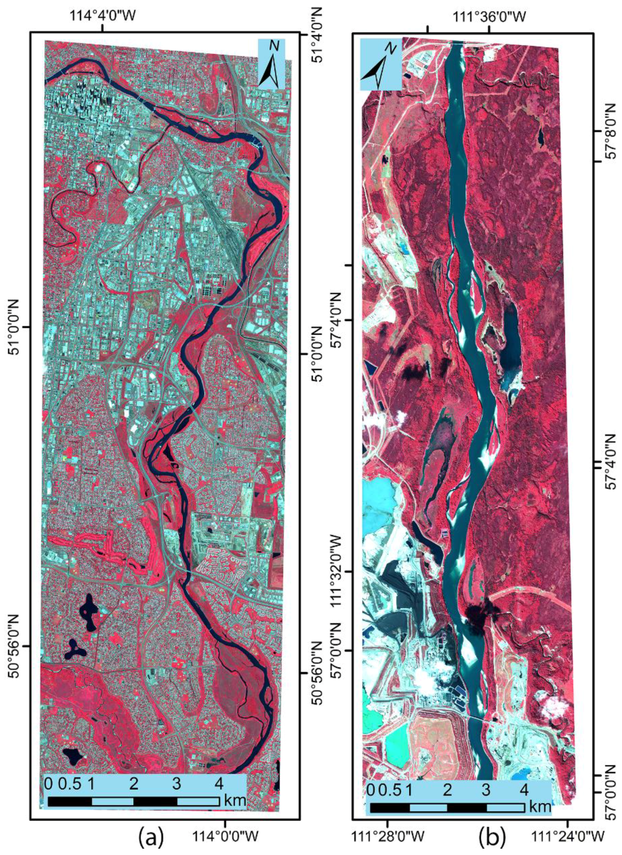
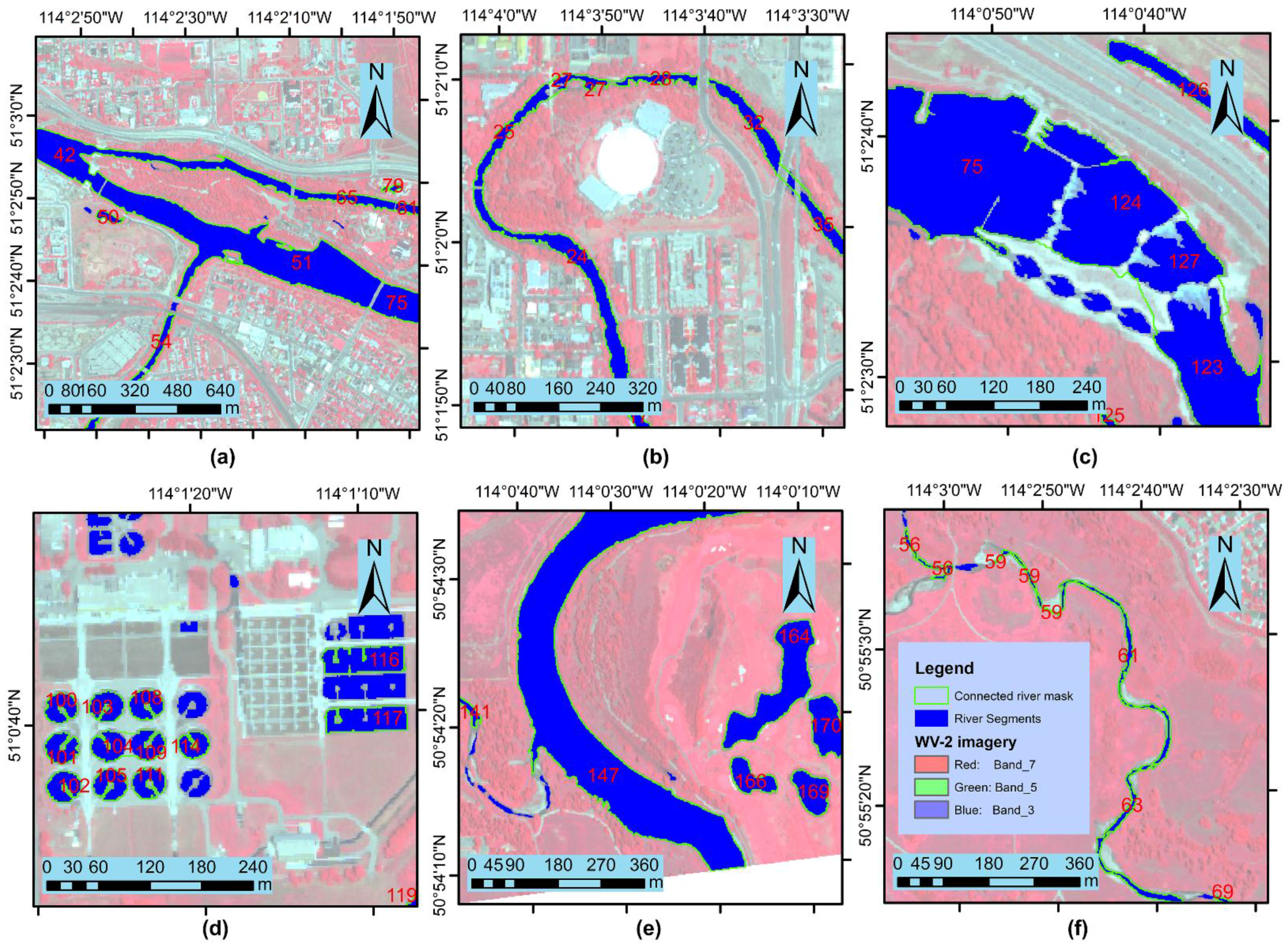
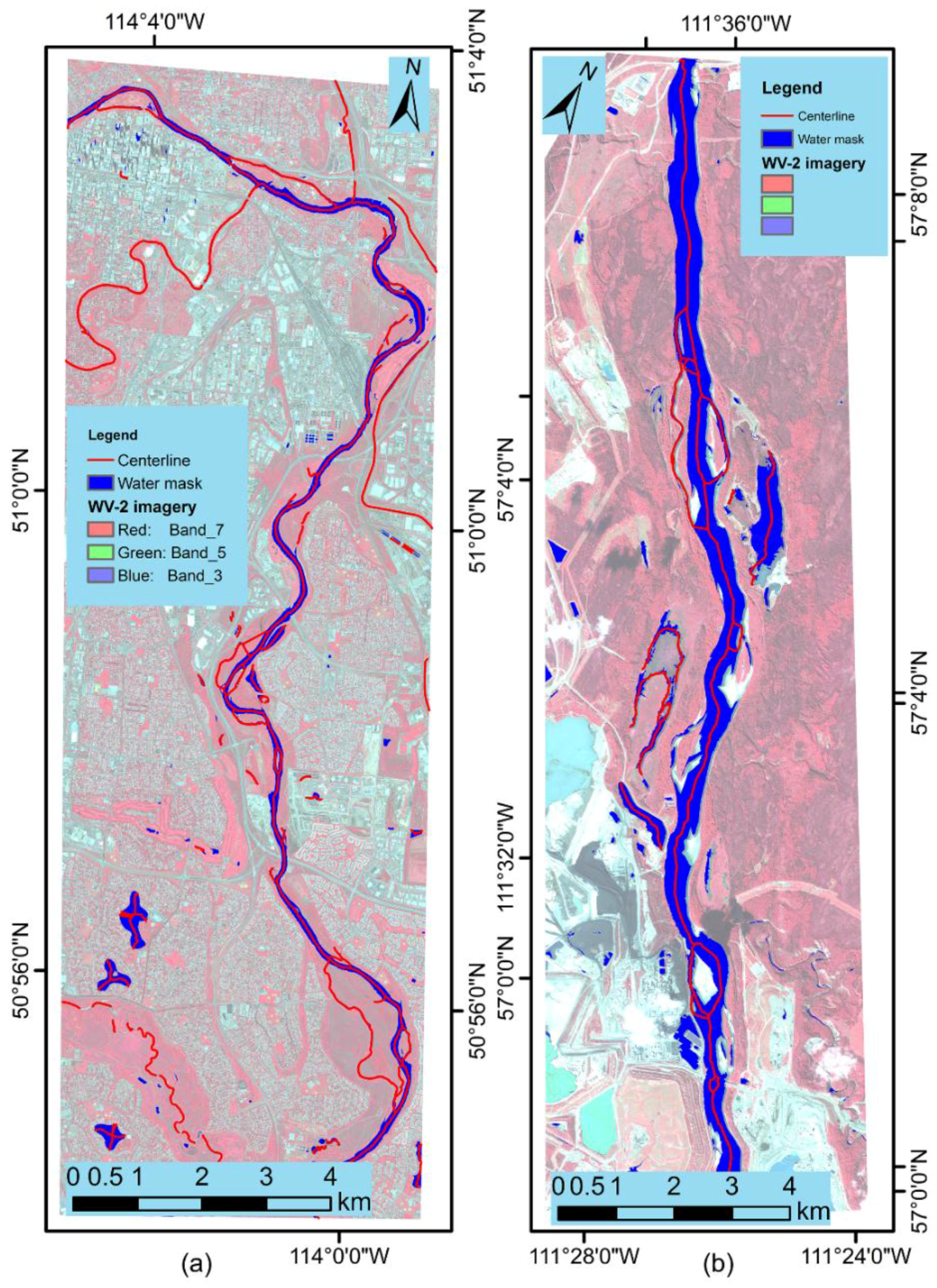
2.1. The Study Site and Imagery

An overview of the study sites of two river sections in Alberta, Canada is given in Figure 1. The first site is the Bow River, which bisects Downtown Calgary, Alberta. It is a typical urban river scene with complex ground features and many bridges over the river. In contrast, the other site of Athabasca River is mainly a natural scene with less human activity. Most experiments are conducted at the Bow River site, while the Athabasca River site is the first of a series of sites that will be used to validate the proposed algorithm. High-resolution Worldview-2 (WV-2) optical imagery was collected at these two study sites. The satellite image parameters are given in Table 1. The false-colour optical images (bands 7, 5, and 3 as R, G, and B, respectively) are shown in Figure 1 for both sites.
Table 1. The specific parameters of input images.
WV-2 ParametersBow River SiteAthabasca River Site
Central location50.973N, 114.036W57.063N, 111.524W
Acquisition time1 August 201213 September 2013
Image size (pixel) *3965 × 90696959 × 9902
Sun elevation angle56.0°36.3°
Spatial resolution1 Pan-band: 0.5m; 8 Multi-spectral bands: 2m
* The image size is the multi-spectral bands at 2 m spatial resolution.

2.2. The Framework of Water Body Detection

The proposed framework of water body detection and connection is designed to solve or mitigate the methodological challenges discussed in Section 1. First, to improve the level of automation, unsupervised classification is adopted where the parameters of image clustering and water class selection will be self-tuning, without subjective training sample collection. Second, to overcome the problem of discontinuous water bodies, a robust river segment connection method is designed to connect river polygons and generate topologically correct rivers. It is comprehensive polygon connection methods according to rivers’ natural attributes. Finally, a refined river centerline method is implemented based on the traditional morphologically method. River polygons are thinned first, edges are organized, and then algorithms are implemented to remove spurs and isolated edges to produce a concise and meaningful river centerline.
The flowchart of the automatic water body detection, connection, and centerline detection is given in Figure 2. In the left column, there are three stages for the water body detection method: (a) initial water body detection from WV-2 stereo imagery pair; (b) water body mask after river connection; and (c) morphological filtering to remove noise and produce a final water mask. With other steps are extensively discussed in existing literature, this paper is focused on the water mask connection stage.
Figure 1. The study sites: The false-colour (band 7, 5, and 3) of WV-2 images for the Bow River site (a) and the Athabasca River site (b). Both river sections are in Albert, Canada.
Remotesensing 07 14055 g001
Figure 2. The flowchart of water body detection and connection.
Remotesensing 07 14055 g002

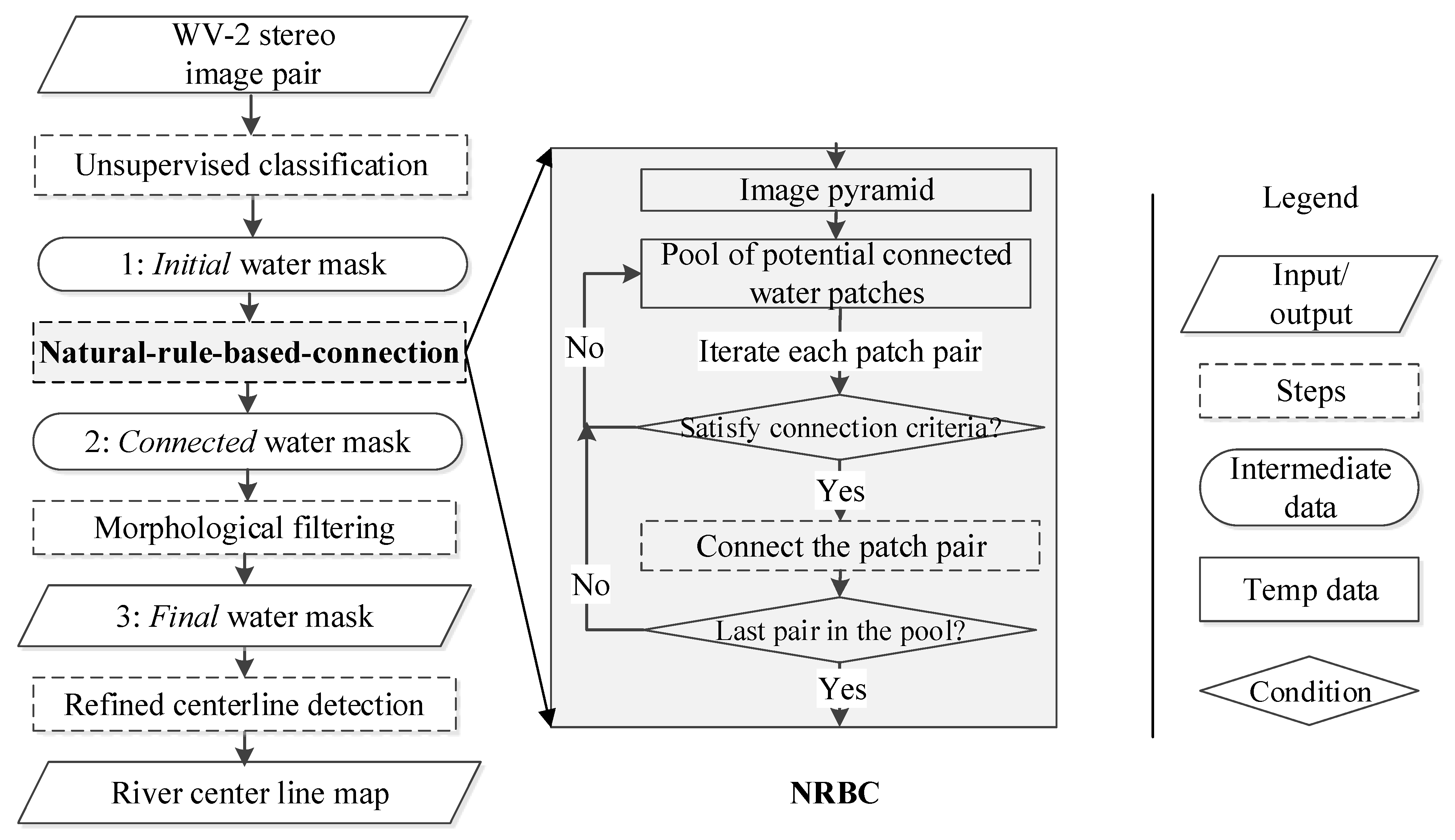
2.3. Unsupervised Classification

As the philosophy of water body detection in this study is to be concise, automatic, and transferable, this study avoids supervised classification or scene-specified rules. A simple unsupervised classification method, the Iterative Self-Organizing Data Analysis (ISODATA) [30], requires only a few parameters as input [23] and it is applied in this study. Unsupervised classification is suitable to separate water from land, due to the unique spectral curve of water vs. other ground features.
After ISODATA clustering, clusters (classes) that represent water are adaptively selected based on physical attributes of water. As water has low reflectance at optical bands, the water classes located close to the origin of the clustering feature space. The adaptive water class selection method searches a small group of classes in the dendrogram [31] that have the shortest individual distances toward the feature space origin. Water is unique in the feature space and usually represented by two to three clusters after ISODATA.

3. Natural Rule Based Connection (NRBC)

With an initial water mask after unsupervised classification, an important task and the focus of this paper is how to connect discontinuous river segments. Natural rule based connection (NRBC) connects discontinuous river segments based on a group of natural rules, with the detailed steps given in middle column of Figure 2. An image pyramid is used to search for candidate pairs of water segments that may connect to each other. For each candidate pair, a series of criteria are tested. A successful candidate pair that satisfies all the criteria will be connected by filling the gap between the pair. After all the pairs are tested and filled (if succeed), a connected water mask is achieved.

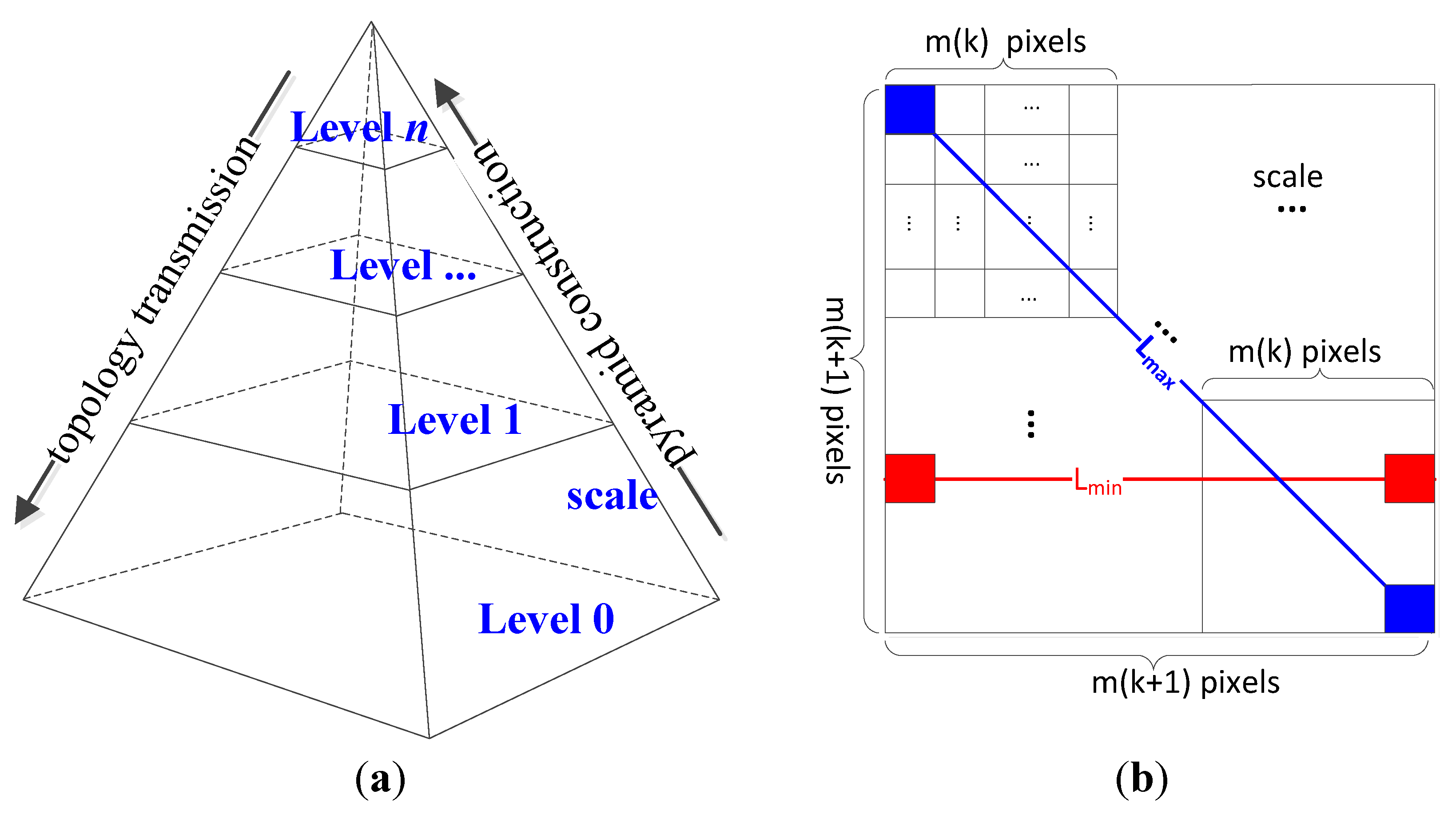
3.1. Image Pyramid Construction

An image pyramid increases pixel (cell) size when moving upward, fills gaps between neighbouring river segments at upper levels, and generates a pool of connectable river segment candidates. A conceptual image pyramid is illustrated in Figure 3a. Given a scale factor (s), an s by s pixel block in current level is aggregated as one pixel in the upper level. After compared with the Gaussian and Laplacian kernels [32], a simple Mean value kernel satisfies the gap connection in this study. The aggregated pixel at upper level is set as 1 if any pixel in the s by s pixel block is 1; otherwise the pixel value is set as 0. The spatial resolution of the image at level k (mk) is given in Equation (1).
As illustrated in Figure 3b, two pixels at level k will be connected in level k+1 if their distance is less than Lmin. They will not be connected if their distance is larger than Lmax. They have a chance to be connected in distance between Lmin and Lmax, depending on their direction difference with pyramid construction direction. The Lmin and Lmax are defined in Equations (2) and (3). It is desirable to design an image pyramid that is expected to fill gaps up to the length of Lmin , with cell size of the top level image equals to or slightly larger than Lmin.
Figure 3. The structure of the image pyramid and the illustration of image resolutions. (a) The image pyramid from level 0 (original water mask) to level n, with scale factor s between each level. (b) The image spatial resolution change from level k to level k+1 in the image pyramid, and minimum and maximum distances that neighbours will be connected at level k+1.
Remotesensing 07 14055 g003
m k = s k
L m i n ( k + 1 ) = m k + 1 = s k + 1
L m a x ( k + 1 ) = 2 L m i n ( k + 1 ) = 2 × s k + 1
The topology of connected segments at the top level of the image pyramid is transmitted to lower levels gradually (mentioned as “topology transmission”). In contrast to the image pyramid construction process, each pixel in the binary mask at level k+1 is assigned to a s by s pixel block in level k. This inverse process is constrained by NDVI [23], where a pixel at level k will not be assigned as potential connectable area if that pixel is dense vegetation. After this inverse process, a new water mask maintains the topology at level n, but with spatial resolution the same as level 0 (original water mask). A pool of potential connectable river segment pairs is detected in this new water mask after image pyramid. Figure 4 is an example of the image “pyramid construction” and “topology transmission” for a part of the Bow River site.
Figure 4. An example of image pyramid construction and topology transmission for river segments. (a)–(c) Image pyramid construction: images at level 0, 2, and 4 with pixel size at 1, 4, and 16 times of the original water mask, respectively; (d)–(f) illustrate river segments topology transmission: the topology of river segments at top level (level 4) in (d) is inherited by images at level 3, level 2 in (e), level 1, and finally to level 0 in (f); and (a,f) have the same spatial resolution.
Remotesensing 07 14055 g004

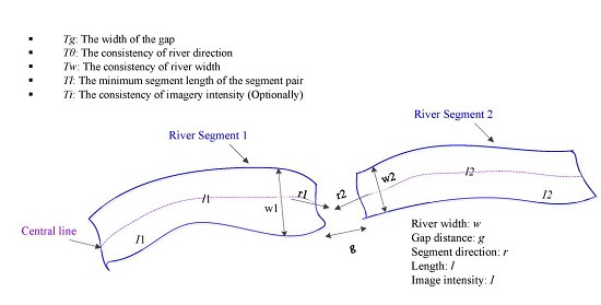
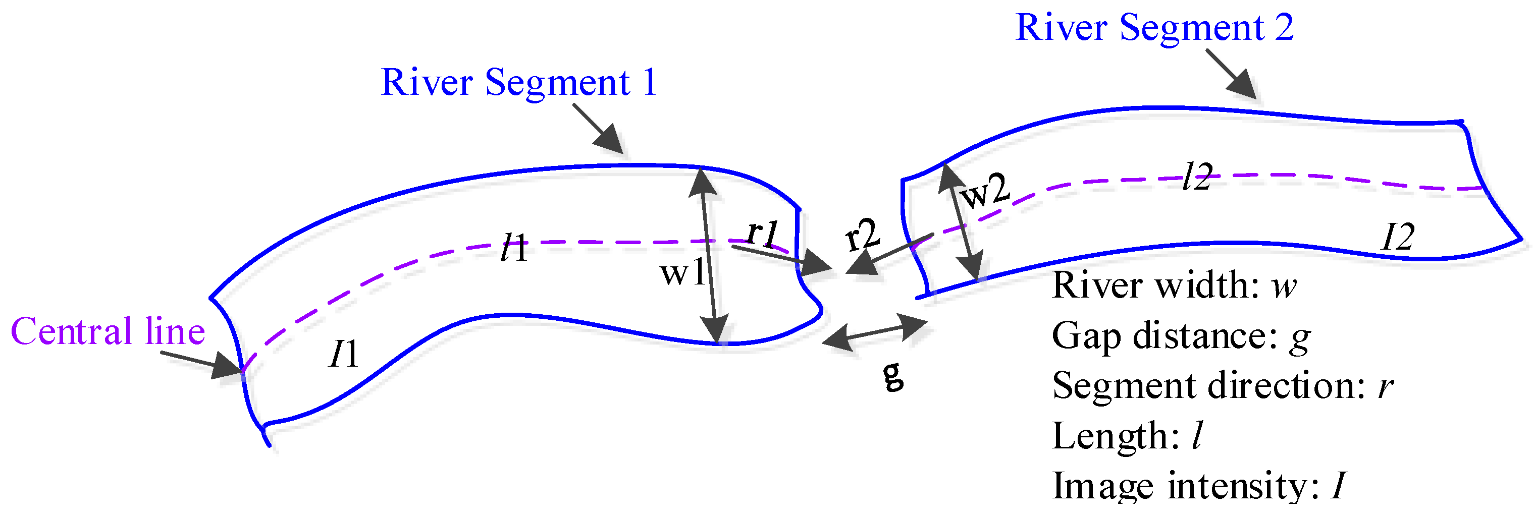
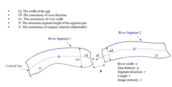
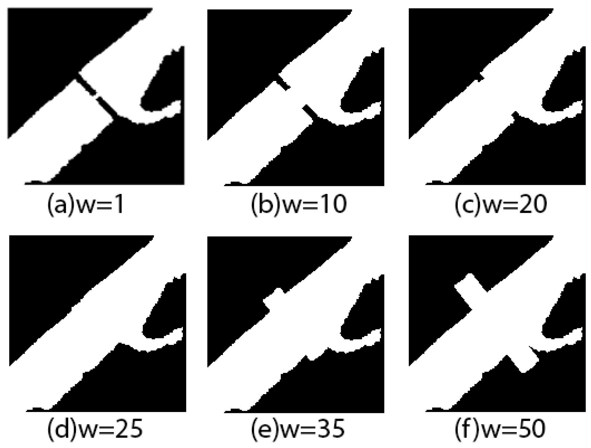
3.2. Rules to Connect River Segments

For each pair of river segments in the pool of potential connectable segments that are adjacent to each other, a set of rules is tested to determine whether that pair of river segments is qualified to be connected. The most popular connection criteria are the centerline direction consistency, the distance (gap) between the two segments, and flow path direction [14,24,25,26]. This study avoids the method dependence on external terrain data, but develops method directly based on the water mask. After evaluating criteria that can infer the consecutiveness of two neighbouring segments, a list of most effective criteria is summarized, as illustrated in Figure 5 and listed as follows:
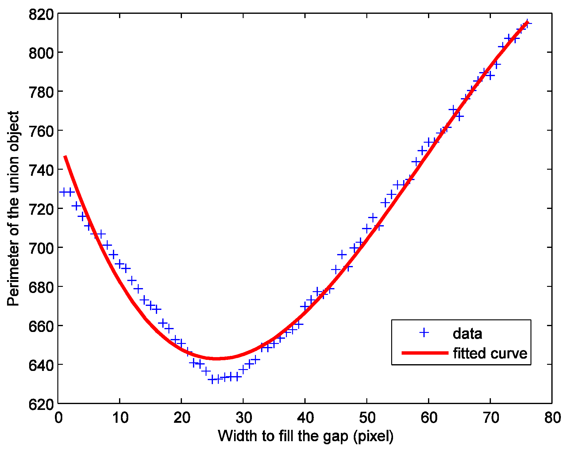
  • Tg: The width of the gap
  • : The consistency of river direction
  • Tw: The consistency of river width
  • Tl: The minimum segment length of the segment pair
  • Ti: The consistency of imagery intensity (optionally)
Figure 5. The conceptual model of river segment connection. The conditions that can infer the consecutiveness of two river segments include the gap width, the river direction consistency, the river width consistency, the minimum river length, and the image intensity consistency.
Remotesensing 07 14055 g005
The gap width between a segment pair should be less than a distance threshold. This distance threshold is applied to image pyramid construction, where segments further than the gap threshold will not be connected at the top level of the image pyramid. Due to the nature of rivers, river channels meander gently in most cases. Thus, two neighbouring segments of the same river should have consistent width and flow path direction. In most cases, rivers are different from other water bodies (e.g., lakes and ponds) and have a long thin shape. A minimum length is used to prevent other water bodies, such as the sewage treatment ponds in Figure 6d from being connected. Finally, neighbouring river segments should appear to be consistent in imagery. The last rule did not apply to this study site, since the first few rules already provided satisfactory results.
Practically, gap width (Tg) is defined before image pyramid construction. Tg is set as 32 m in this study; then an image pyramid with 5 levels (from level 0 at bottom to level 4 at top) with scale factor 2 is built according to Equation 1. Tg may require slight adjustments to satisfy different image scenes and image resolutions. River segment direction difference () is set as 90°, based on the assumption that two neighbouring river segments will have channel direction change that is less than a right angle. The segment width consistency threshold (Tw) is given by the ratio of maximum width and minimum width of the two segments, given in Equation (4). As the width may vary along a river segment, the average width near the broken end is used to represent a segment’s width. The ratio for Tw is set as 3 in this study, which means the maximum and minimum width should be less than three times. The minimum length threshold (Tl) relies on the gap width between the pair, and the minimum length of a segment along the centerline direction should at least double the length of the gap, as defined in this study. Finally, the intensity difference (Ti) can be defined as the Mean or Mahalanobis distance [23] of image intensity between two segments, where intensity can be colour in optical imagery or backscatter value in SAR imagery. A pair is labelled as connected only if it satisfies all the rules at the same time.
T w = max ( width 1 , width 2 ) min ( width 1 , width 2 )
Example scenarios of river segments from the Bow River site are given in Figure 6. There are simple scenarios, where river segments are broken down by bridges and dams, with consistent direction and width, such as in Figure 6a,b. There are also complicated cases, where river segments are broken down by waves or noise, with problematic centerlines and misleading directions, such as in Figure 6c. There are even some cases of non-continuous rivers, such as the sewage treatment ponds in Figure 6d. The proposed NRBC method can tackle complex cases such as in Figure 6c, where pixel-level tracing method relied on the centerline will be invalid.
Figure 6. Four examples of river segment connection scenarios. The blue mask is the river segments, while the over-draped red lines are centerlines extracted from the new water mask after image pyramid. (a) and (b) Simple scenarios: river segments discontinued by bridges; (c) Difficult scenario: river segments discontinued by a dam and waves; (d) Incorrected scenario: sewage treatment ponds.
Remotesensing 07 14055 g006

3.3. River Segment Connection Method

If a segment pair successfully passes all criteria and is qualified to be connected, the gap between the two segments is filled using a region growth strategy. The two segments can be connected by the centerline after image pyramid and topological transmission. The centerline pixels in the gap are used as seeds to grow and fill the gap. As shown in Figure 7, a connected river segment includes the two original river segments and the growing centerline object filling the gap. As shown in Figure 8, the perimeter of this connected river segment will first decrease then increase after it reaches a perimeter minima point. The growing centerline first fills the gap and reduces the perimeter until the width of the centerline object equals the width of the river itself, as illustrated in Figure 7a–d. After this perimeter minima point, the perimeter increases due to the growing width expanding out of the gap, as in Figure 7e–f. The perimeters associated with each centerline width produces a curve given in Figure 8. A local minimum in Figure 8 represents the point where the centerline growing width is close to the river width. To make the curve’s local minimum more stable, a fitted curve is used to replace the discrete values. The perimeter is minimized at the optimal width for simple scenarios. In complex scenarios with distracting factors that will generate a perimeter length curve with multiple local minimums, either the first local minimum or the overall minimum is selected, according to their corresponding shape similarity between filled area and the image pyramid.
Figure 7. The growing centerline width to fill the gap between a river segment pair, with the centerline grows from width 1 (original mask), 10, 20, 25 (ideal width), 35, and 50 pixels in (a)–(f), respectively.
Remotesensing 07 14055 g007
Figure 8. The perimeter of the connected river segment changes as the gap been filled with growing width centerline. The data in this Figure is related to Figure 7.
Remotesensing 07 14055 g008

4. Post-Processing and River Centerline Extraction

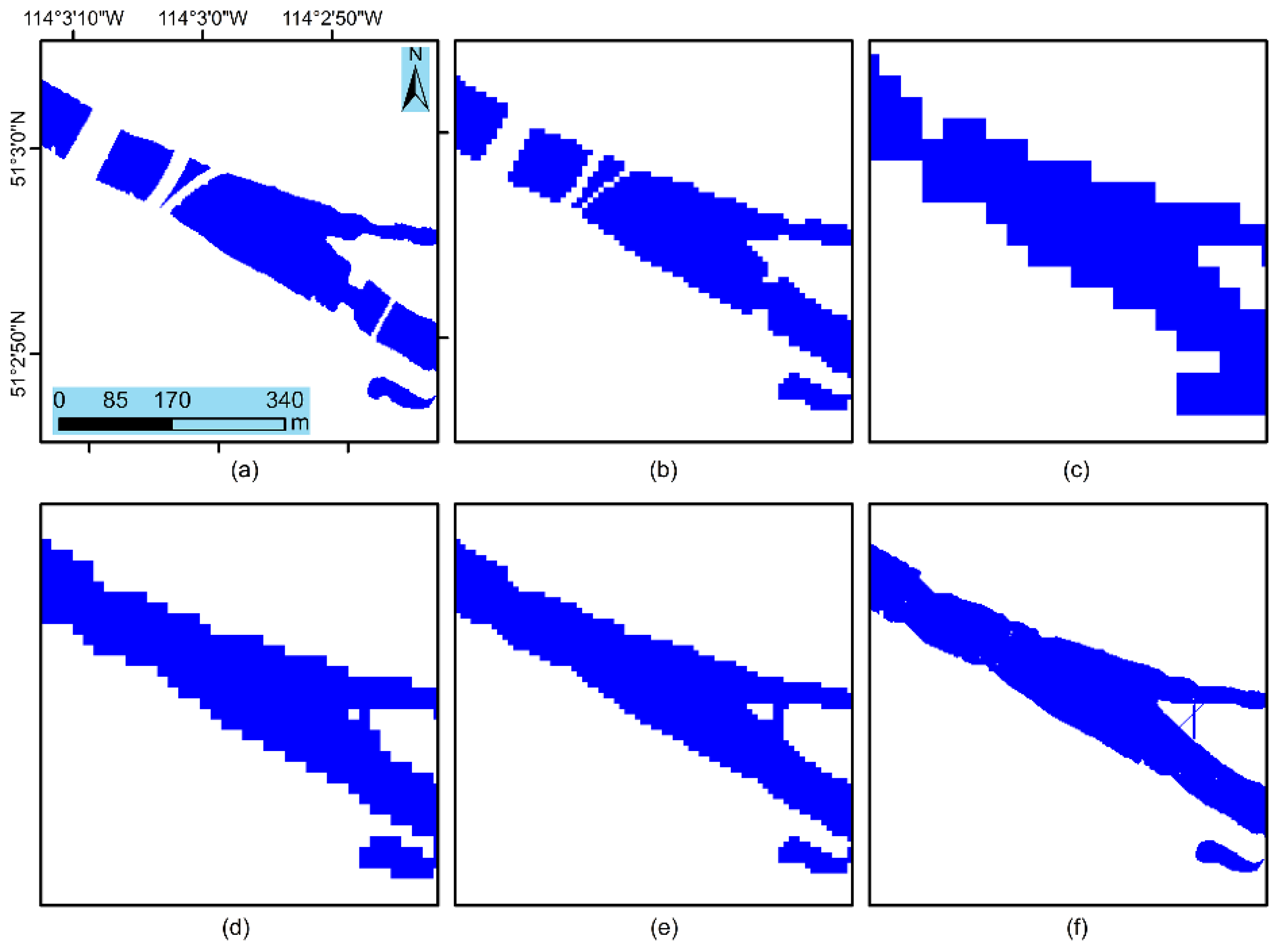
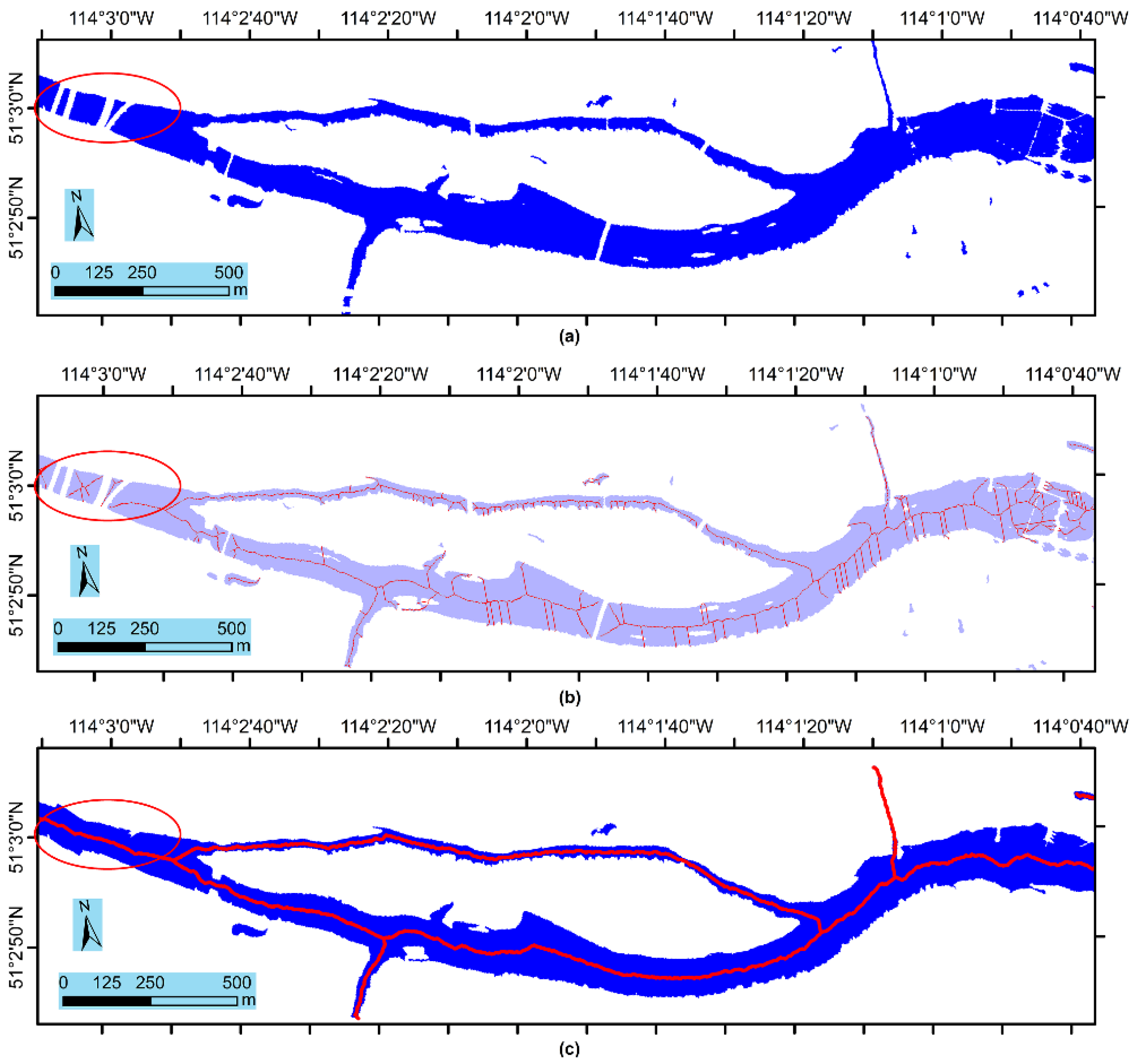
4.1. The Final Water Mask after River Segment Connection

After river segment connection, path opening or closing morphological filtering [33] is employed to generate the final water mask. The morphological direction path open and close filters use a set of four different adjacency graphs corresponding to the four classical orientations as four structuring elements: one graph for horizontal lines, one that produces approximately vertical lines, and two that create approximately diagonal lines. According to these four adjacencies, path opening is equivalent to the supremum of all the openings. Furthermore, a final optional step is to apply a minimum area constraint (Area < 25 m2 in this case) and to remove tiny segments and clean the water mask.
Figure 9. Centerline extraction and refinement using the morphological algorithm: (a) The water mask before river segment connection; (b) The centerline after thinning the refined water mask using morphological methods. This centerline is discontinuous and has many spurs; (c) The centerline extracted from the final water mask by thinning polygons and cleaning the spurs, over-draped on the final water mask.
Remotesensing 07 14055 g009

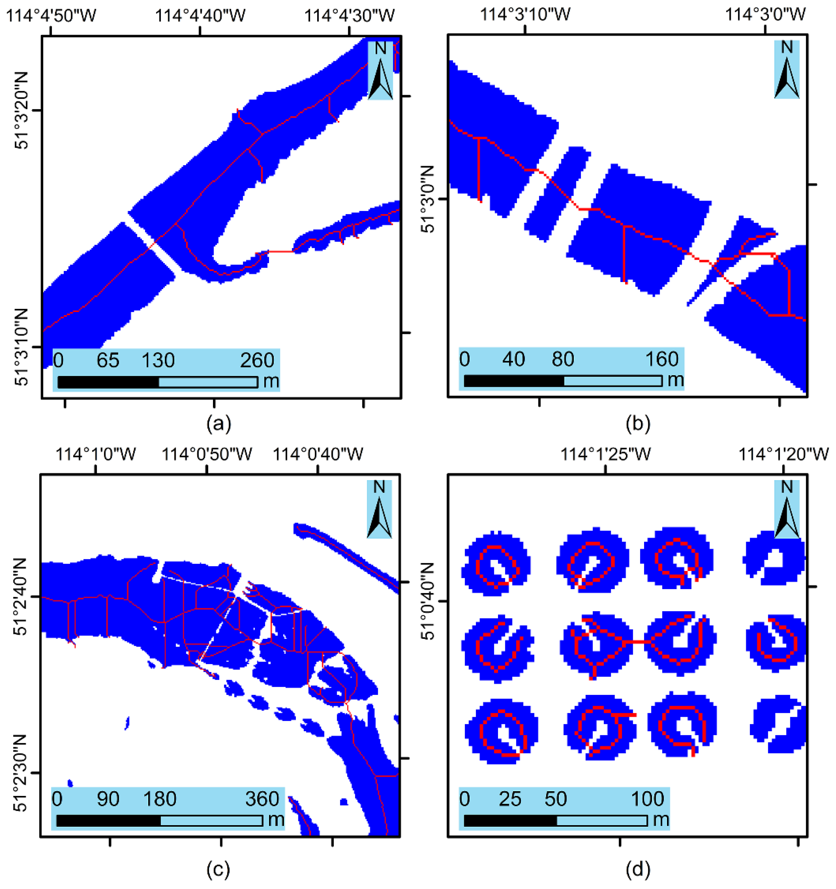
4.2. River Centerline Extraction

An accurate river centerline can be extracted from continuous rivers in the final water mask. Traditional morphological methods [28] thin and skeletonize the water mask and generate a river centerline that possesses many irrelevant branches that weaken the conciseness and effectiveness of the centerlines. This study proposes a method to refine the centerline by organizing the edges first and then remove spurs using conditions.
Small holes inside river segments are filled in the final water mask, because small holes change the topology and increase irrelevant edge links. We adopted the edge cleaning method published in Kovesi [34], where isolated edges and spurs that are shorter than a minimum length are removed, after building a network of edges. In this study, the minimum length of edge was set as two-thirds of the average river width, because spurs usually has a length close to half of the river width.
As illustrated in Figure 9, a water mask before river segment connection in Figure 9a has discontinuous segments and small holes inside the river extent. The traditional morphological method directly applied on this mask produces a problematic river centerline, as shown in Figure 9b. It is noticeable that the river centerlines are broken down and have many spurs. In Figure 9c, the morphological algorithm is applied to the final water mask. An edge network is built to define their connectivity and topology, spurs shorter than two-thirds of the average river width are removed, and the final centerline is created. The one-pixel raster format centerline is further converted to a vector polyline for easier operation in hydrological applications.

5. Results and discussions

5.1. Unsupervised Classification Accuracy

The reference water mask is digitalized based on the classification result water mask, with water polygons been added, deleted and edited. The pan-sharpened optical image with four time’s higher spatial resolution than that of the resultant layers is used as the reference layer for digitization. During the digitalization, the archived Google Earth aerial images are used as guidance to distinguish water from land. There are 1,075,210 reference water pixels for the Bow River site. The resulting accuracy for each input band combination is compared in terms of their user’s accuracy, producer’s accuracy [23], and Quality [35], as shown in Table 2.
  • User’s accuracy (UA) = overlapped area/detected water area
  • Producer’s accuracy (PA) = overlapped area/reference water area
  • Quality (Q) = overlapped area/(detected water area + reference water area − overlapped area)
Table 2. The unsupervised classification accuracy of different input bands at the Bow River site.
Methods UAPAQ
ISODATA95.3%96.1%91.7%
MNDWI (threshold: 0.45)88.7%67.8%62.4%
From Table 2, the accuracy (Q) of unsupervised classifications is 20% higher than direct thresholding MNDWI, which suggests that unsupervised classification outperforms direct thresholding for water body detection. A comparison with different input bands for classification, such as images after atmosphere correction, image pan-sharpening, and external DEM, also report very similar accuracy as the raw WV-2 bands. As a result, the unsupervised classification with raw bands was applied in this study and 91.7% water mask accuracy guarantees the further river connection is based on reliable input river segments.

5.2. Qualitative Analysis of NRBC

Figure 10 provides six scenarios after river segment connection to analyze the performance of NRBC. These six scenarios are the results generated using the default criteria values. Figure 10a is a typical case for discontinuous situations, where a river is broken down by man-made infrastructures (bridges, dams, pipelines, etc.) in urban areas. Bridges with different width and direction were successfully connected. NRBC performs well on such typical cases because the neighbouring river segments have highly consistent width and direction (e.g., segment pair 42/65, 51/75). One segment pair 51/54 failed to be connected because the two bridges are located very close to each other, the small river segment between these two bridges was missed in the image classification, and NRBC did not connect this pair due to the large gap. From the shape of the connected river boundaries, gaps between segments are appropriately filled without abrupt width change at the gaps.
Figure 10b demonstrates the performance of NRBC’s default values applied to a narrow tributary of the river. Gaps between segment series 17/24/25/27/28 and segment series 32/35/36 were all successfully handled. The gap between segment 32 and 35 was a two-bridge-crossing situation and NRBC made an appropriate connection. The gap between segment 28 and 32 was not processed because it does not fulfill the minimum segment length (Tl) criterion. An additional iteration of NRBC will make this connection. Figure 10c showed a dam that produced waves and broke the river into segment series 75/124/127/123 in the image. It is difficult to connect these irregular shape segments using pixel-tracing methods, however, NRBC successfully connected these segments using the rules at polygon-level. Figure 10d shows a case where water segments should not be connected. The minimum segment length (Tl) criterion was used by NRBC to separate thin-long-shaped river and these round-closed-shaped sewage treatment ponds. In Figure 10e, ponds are correctly kept intact during the connection due to the same criterion as Figure 10d. Segment pair 141/147 was not connected because the tributary is too narrow and part of the very thin tributary was missed during the water mask detection. Thus an accurate water mask is critical for NRBC.
Finally, Figure 10f shows that NRBC has limitations for the detection of the narrowest upstream tributary (one or two pixels wide). The narrow river channels were not well-detected in the initial water mask because of mixed pixels, shallow water, narrow channels, or overhung trees. This led to many gaps in surface water polygons, which challenged NRBC. Furthermore, the highly sinuous tributary has abrupt changes in direction, which also reduced the ability of NRBC to make the appropriate connections. The NRBC method performed best when the river width was many times the pixel resolution. Higher resolution imagery may improve classification of ‘narrower’ rivers. Alternatively, a different set of NRBC parameters can be used to connect small rivers.
Figure 10. Six diverse cases of NRBC river detection. The blue extracted river segments are draped on the false-colour WV-2 imagery. The green polylines show the connected river boundaries after application of the NRBC algorithm. (a) Typical river segments that are successfully connected; (b) Connection at a narrow stream; (c) A complicated segment connection case at the dam; (d) and (e) Ponds are not connected based on minimum segment length rule; (f) The narrowest upstream misses some connections due to input water mask limitation.
Remotesensing 07 14055 g010

5.3. The Sensitivity of Criteria in NRBC

The influence of the four major criteria used in NRBC was investigated. The connected water mask of Bow River site had 179 river segments of four-connected regions. Based on knowledge of the river system, fifty-seven pairs of these water segments should be connected. The following symbols were defined to quantitatively analyze the performance of NRBC:
  • “T→T”: for a pair of river segments set as “should be connected (T)” by visual inspection, it is connected (T) in the experiment.
  • “T→F”: for a pair of river segments set as “should be connected (T)” by visual inspection, it is not connected (F) in the experiment.
  • “F→T”: for a pair of river segments set as “should not be connected (F)” by visual inspection, it is connected (T) in the experiment.
The corresponding UA, PA, and Q were then defined in a similar way as described in Section 5.1. For example, “T→T” corresponds to “overlapped area”. To test the sensitivity of each criterion, a range of values for each criterion was processed in NRBC. The corresponding connected water segments were then evaluated against visual inspection. When one criterion was tested, other criteria were kept as default.
The gap width threshold (Tg) influenced both the image pyramid construction and later segment connection. We tested image pyramids built using popular scale 2 with level 3 to 8. In Table 3, medium Tg produced the highest consistency with ground-truthed connections, according to Q values. A low Tg value is not sufficient to fill gaps and build connections between neighbouring river segments, whereas a large Tg value typically connected irrelevant segments far from each other. An appropriate Tg value is the maximum length of obstacles over rivers. Practically, Tg is suggested to double or triple the maximum obstacle width because of direction variance described in Figure 3b and some extreme cases such as two close bridges described in Figure 10a,b. For instance, Table 3 suggests that 90 m (45 pixels in 2 m spatial WV-2 imagery) is an appropriate Tg for this site since most obstacles over rivers in this scene are bridges, which are less than 50m wide.
Table 3. The sensitivity of gap width (Tg) in NRBC.
Image Pyramid (scale ^level)Gap Width (pixels)T→T *T→FF→TUAPAQ
2 ^3113126391.2%57.4%54.4%
2 ^4224413393.6%81.5%77.2%
2 ^545516394.4%94.4%89.5%
2 ^690516394.4%94.4%89.5%
2 ^7181507394.3%92.6%87.7%
2 ^8362507394.3%92.6%87.7%
* There are 179 river segments and 57 pairs should be connected based on ground truth data. The gap width is 2 × s c a l e l e v e l according to Equation 2. The definition of “T→T”, “T→F”, and “F→T” is given in Section 5.3. The definitions of UA, PA, and Q are provided in Section 4.1.
Table 4. The sensitivity of river direction () in NRBC.
Direction Angle (°)T→T *T→FF→T UAPAQ
304017295.2%74.1%71.4%
404413295.7%81.5%78.6%
50489296.0%88.9%85.7%
60507394.3%92.6%87.7%
70507394.3%92.6%87.7%
80507394.3%92.6%87.7%
90516394.4%94.4%89.5%
100516394.4%94.4%89.5%
* Please see the footnote of Table 3 for column definitions.
The sensitivity of constraint on the direction consistency (Tθ), the allowed direction angle change between two connectable segments, was tested (Table 4). In this study site, increasing the direction angle tolerance led to a slight performance in improvement, with respect to the Q values. When Tθ > 45°, NRBC generated a good result. A further increase in angle contributed to a mere 3.8% increase of Q. The curvature relative to the pixel size is important for Tθ. In most cases, the angle of directional change between two river polygon segments is less than a right angle (90°).
The sensitivity of the consistency of width between the two adjacent segments (Tw), expressed as the ratio of the wider segment to the narrower segment, were tested over a range of values from 1.5 to 5 (Table 5). With a small Tw, two neighbouring segments must have similar width to be connected. With large Tw values, connects can be made between river channels with dramatic changes in width. Increasing Tw led to slightly improving performance. Increasing Tw also introduces the risk of incorrectly connecting segments in some situations (e.g., narrow river segments and wide nearby ponds). For river flows along moderate or low terrain relief without dams, a default ratio of 3 for Tw is appropriate.
Table 5. The sensitivity of max-min width ratio (Tw) in NRBC.
Width Ratio (max/min)T→T*T→FF→TUAPAQ
1.54512197.8%83.3%81.8%
2489296.0%88.9%85.7%
2.5516296.2%94.4%91.1%
3516394.4%94.4%89.5%
3.5516394.4%94.4%89.5%
4525394.5%96.3%91.2%
4.5525394.5%96.3%91.2%
5525394.5%96.3%91.2%
* Please see the footnote of Table 3 for column definitions.
The minimum segment length along centerline direction (Tl) constraint was expressed as the ratio of segment length along centerline direction to the gap width. A range of Tl values were tested (Table 6). The performance of the NRBC algorithm first increases and then decreases with the growing Tl in this study site. The best performance (i.e. highest Q value) was associated with a Tl value of 3.5. With a small Tl, short segments were accepted and there is the risk to connect other water bodies such as ponds. If Tl is too large, connections may not be made in urban areas where rivers are bisected by many bridges. Successive iterations of the NRBC algorithm with a small Tl value can be used to connect river segments in these urban cases.
Table 6. The sensitivity of minimum segment length (Tl) in NRBC.
Min Len Ratio (Seg/gap)T→T *T→FF→TUAPAQ
1516689.5%94.4%85.0%
1.5516591.1%94.4%86.4%
2516394.4%94.4%89.5%
2.5507296.2%92.6%89.3%
3507296.2%92.6%89.3%
3.5507198.0%92.6%90.9%
44512197.8%83.3%81.8%
4.54413197.8%81.5%80.0%
54215197.7%77.8%76.4%
* Please see the footnote of Table 3 for column definitions.

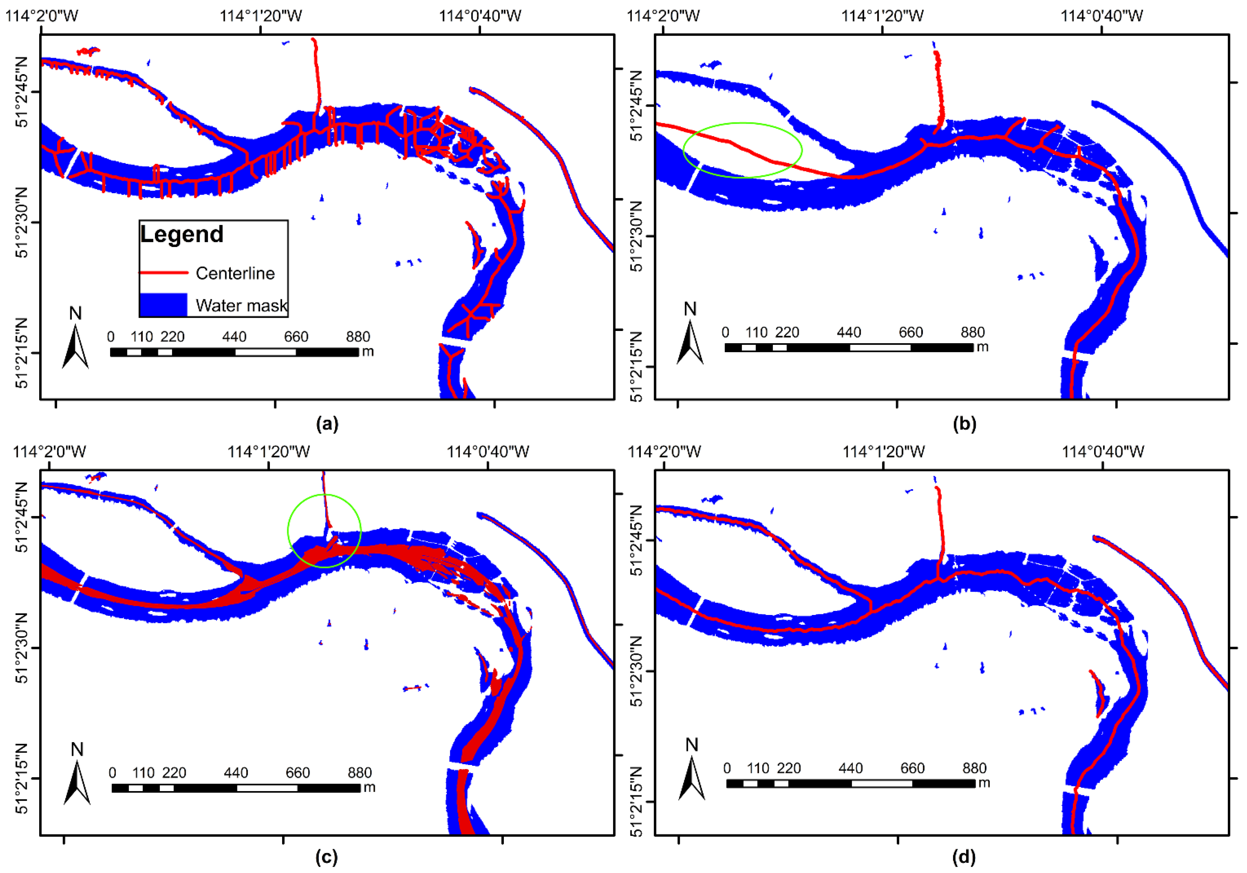
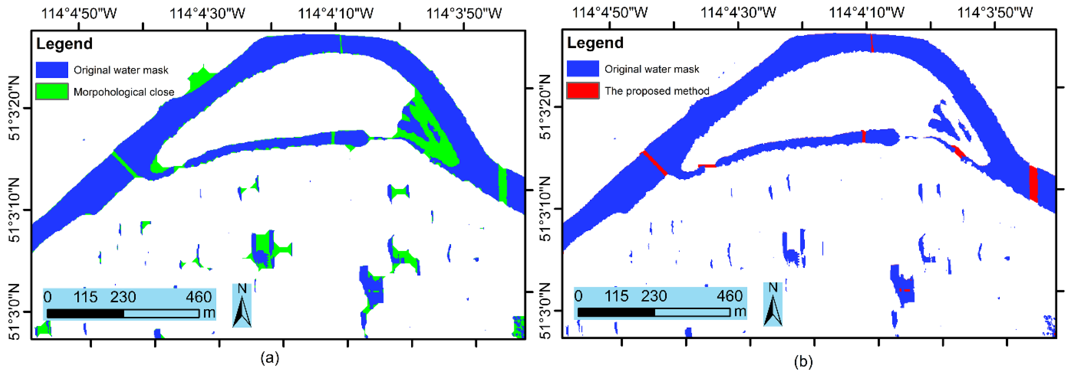
5.4. Comparison 1: River Segments Connection

Discontinuous river segments were connected using the proposed NRBC method at the polygon-level. To evaluate the performance of NRBC, we compared it with a traditional morphological method, which connects binary objects using a morphological close operation. The pixel-based centerline connection methods described in the introduction are not comparable to the NRBC method because they were working on pixel-wide rivers. Pixel-based methods process different units (centerline and vertexes) using different strategies compared to the NRBC method. The comparison of the morphological method and the NRBC method on a section of Bow River connection is given in Figure 11.
Figure 11. The comparison of river connection using (a) the morphologic algorithm and (b) the NRBC method. The morphometric method mistakenly connects shadows and noise segments The NRBC method selectively connects only meaningful river segments based on its rules.
Remotesensing 07 14055 g011
The advantage of the NRBC method over the morphologic method is that NRBC considers the attributes of rivers (rules) during the connection. The rules guarantee that the connecting is meaningful in the real world, whereas the morphologic close operation connects any segments after defining the structuring element. As illustrated in Figure 11, gaps between noises, shadows, concave riverbanks, or fork-shape wetted areas are all filled after morphological close operation. In contrast, NRBC merely fill the gaps that are actually broken down river segments, as shown in Figure 11b. The few pixels in the shadow located at the bottom-right side of Figure 11b are filled during pre-processing and whole-filling, not during the connection stage.

5.5. Comparison 2: River Centerline Extraction

To evaluate the centerline extraction method proposed in this study, two other centerline extraction methods are compared and analyzed. The most popular centerline detection method is the morphological method [28], where pixels at the edge of an object are iteratively deleted until a single-pixel width centerline. Morphological methods preserve the topology of the original water mask but keep many irrelevant branches. Another method is the Mean-shift [36] method, which was designed for road centerline detection. The Mean-shift method iteratively shifts each point x to the average m(x) of all neighbouring points until a stable stage, where average m(x) is given by:
m ( x ) =   1 n x i N ( x ) x i
where N(x) is a set of neighbouring points of x, and n is the number of points within N(x). The comparison of these three methods on a section of Bow River site is given in Figure 12.
RivWidth method calculated the distance from each river pixel to the nearest land pixel, and then the ridge of the high distance value along the river mask was used to search for a centerline [37]. The Mean-shift method works in a very different manner, shifting points (pixels) onto the center of its neighbouring pixels. The proposed method, which is based on the morphological method, cleans all irrelevant spurs to give a concise and accurate expression of the river. It also addresses the problem with loops in the centerline.
The morphological method generates the centerline with many spurs (Figure 12), which dampen the effectiveness of the method, because spurs are noise for hydrological applications. Methods (a), (c), and (d) work well on the thin continuous canal on the upper-right of the scene. That is because this canal is continuous, complete, with no branches, and without distractive neighbouring water segments. However, the three methods perform differently when processing the wider and more complicated main river in the center of the scene. The RivWidth method was not designed to be accurate on rivers with islands or multi-channels as highlighted in the green circle in Figure 12b. RivWidth did not process narrow tributaries and the canal as well, mainly because it was focused on the main channel. Mean-shift Method fails to extract centerline for wide and narrow rivers simultaneously, because the definition of neighbour size affects the aggregating distance. As in Figure 12c, when the canal centerline is correctly extracted, the wider main river’s centerline does not aggregate well. Moreover, at the point where two rivers converge, as circled in the center of the Figure 12c, the averaging strategy of Mean-shift produces a centerline inside neither of the two rivers, but appeared as a compromise of both rivers. In Figure 12d, the processed method extracts an accurate and concise centerline for main channel, its tributaries, and the canal.
Figure 12. The comparison of river centerline extraction methods over a section of the Bow River site: (a) morphological method; (b) the RivWidth method described in [37]; (c) the Mean-shift method described in [36]; and (d) the proposed method.
Remotesensing 07 14055 g012

5.6. The Final Water Mask and River Centerlines

The detected final water masks and centerlines for both study sites are given in Figure 13, in large image areas of urban and natural scenes. The minor error of water body mask at the Bow River site is mainly due to the mixture between water and some shadows in the urban area. In the Athabasca River site, the trivial confusion comes from areas of mined bitumen, where the dark sands appear to have similar colour and backscatter signature as deep water.
The extracted centerlines describe the rivers in a topologically corrected form, which is an important improvement from discontinuous segments after image classification. At both sites, the river centerlines are extracted correctly from one end to the other, without unnecessary short branches (“spurs”). The Bow River is narrower than the Athabasca River in the given scenes, but the centerline detection method performs stably on both of them. There are more bars inside the Athabasca River, thus the centerline make rings accordingly to keep the river channel’s topology.
Figure 13. Final water masks and river centerlines for (a) the Bow River site and (b) the Athabasca River site. The background is the false colour optical images using WV-2 bands. The final mask (blue colour patches) and the river centerlines (red lines) are draped over the background.
Remotesensing 07 14055 g013

6. Conclusions

In this study, we addressed issues relating the automatic detection of water bodies and their assemblage into a continuous river polygon using a hierarchically structured polygon connection algorithm. The water mask after classification, with an overall accuracy of 91.7%, was used as input for river segment connection. A new method to connect river segment at the polygon level, “natural rule based connection (NRBC)”, was designed based a series of criteria including gap width between river segments, minimum length of river segments, and the consistency between river segments’ direction and width (Figure 5).
The analysis of six river network connection scenarios using NRBC (Figure 10) illustrated the necessity of the four criteria, and the effect of an input water mask’s accuracy and spatial resolution on NRBC. The sensitivity analyses (Table 3, Table 4, Table 5 and Table 6) demonstrated that the gap width (Tg) and minimum segment length (Tl) had an inverted U-shaped curve with respect to the increasing criterion value, the increasing direction tolerance (Tr) improved the NRBC performance, and the increasing max-min width ratio (Tw) generally enhanced NRBC but with some exceptions in this study. The default criteria for a general river were suggested as: two or three times of the maximum obstacle width for Tg, a right angle tolerance (90°) for Tr, and around two or three for Tw and Tl. In comparison with the morphological close algorithm (Figure 11), this proposed NRBC connected the river segments correctly, but the noise, shadow, and unrelated water segments remain unchanged. Moreover, the comparison of centerline extraction method proposed in this study with three other methods (Figure 12) exhibited that the proposed method produces complete but concise centerlines for rivers and maintains topology when gravel bars create flow bifurcations and junctions.
The detected river inundation layer and extracted river centerlines provide a valuable data source for mapping flood extents, validating hydraulic models for the assessment and management of water quality, quantity and aquatic habitat. The delineation of an accurate water mask is also a pivotal step in riverine feature extraction (i.e. bridges and dams) algorithms. Collectively, these data products can help provide data for the improved management of both the rivers and the adjacent water bodies. The proposed NRBC method can be adapted for other polygon-shape feature connection (e.g., roads) after detection from remotely sensed data, with specific rules needs to be modified.

Acknowledgments

The work is undertaken with the financial support of the Canadian Space Agency and the MITACS Accelerate Program. We would also like to thank the anonymous reviewers for their constructive comments and feedback to improve the quality of this paper.

Author Contributions

Chuiqing Zeng contributed to the research design, algorithm development, experiment analysis, and manuscript writing. Stephen Bird supervised this study, collected imagery, provided suggestions during experiments, and contributed to manuscript editing. James J. Luce and Jinfei Wang are advisors of this study and contributed to group discussions and manuscript editing.

Conflicts of Interest

The authors declare no conflict of interest.

References

  1. Becker, M.; da Silva, J.S.; Calmant, S.; Robinet, V.; Linguet, L.; Seyler, F. Water level fluctuations in the congo basin derived from envisat satellite altimetry. Remote Sens. 2014, 6, 9340–9358. [Google Scholar] [CrossRef]
  2. Ghoshal, S.; James, L.A.; Singer, M.B.; Aalto, R. Channel and floodplain change analysis over a 100-year period: Lower yuba river, California. Remote Sens. 2010, 2, 1797–1825. [Google Scholar] [CrossRef] [Green Version]
  3. Khan, S.I.; Hong, Y.; Gourley, J.J.; Khattak, M.U.; de Groeve, T. Multi-sensor imaging and space-ground cross-validation for 2010 flood along indus river, Pakistan. Remote Sens. 2014, 6, 2393–2407. [Google Scholar] [CrossRef] [Green Version]
  4. Chen, L.; Michishita, R.; Xu, B. Abrupt spatiotemporal land and water changes and their potential drivers in poyang lake, 2000–2012. ISPRS J. Photogramm. Remote Sens. 2014, 98, 85–93. [Google Scholar] [CrossRef]
  5. Ghosh, M.K.; Kumar, L.; Roy, C. Monitoring the coastline change of hatiya island in bangladesh using remote sensing techniques. ISPRS J. Photogramm. Remote Sens. 2015, 101, 137–144. [Google Scholar] [CrossRef]
  6. Smith, L.C. Satellite remote sensing of river inundation area, stage, and discharge: A review. Hydrol. Processes 1997, 11, 1427–1439. [Google Scholar] [CrossRef]
  7. Frazier, P.S.; Page, K.J. Water body detection and delineation with landsat TM data. Photogramm. Eng. Remote Sens. 2000, 66, 1461–1467. [Google Scholar]
  8. Rodríguez-Cuenca, B.; Alonso, M.C. Semi-automatic detection of swimming pools from aerial high-resolution images and lidar data. Remote Sens. 2014, 6, 2628–2646. [Google Scholar] [CrossRef]
  9. Xie, H.; Luo, X.; Xu, X.; Tong, X.; Jin, Y.; Pan, H.; Zhou, B. New hyperspectral difference water index for the extraction of urban water bodies by the use of airborne hyperspectral images. J. Appl. Remote Sens. 2014, 8. [Google Scholar] [CrossRef]
  10. Schumann, G.; Baldassarre, G.D.; Bates, P.D. The utility of spaceborne radar to render flood inundation maps based on multialgorithm ensembles. IEEE Trans. Geosci. Remote Sens. 2009, 47, 2801–2807. [Google Scholar] [CrossRef]
  11. Li, X.; Liu, X.; Liu, L.; Xue, K. Comparative study of water-body information extraction methods based on electronic sensing image. In Advances in Mechanical and Electronic Engineering; Springer Berlin Heidelberg: Berlin, Germany, 2013; pp. 331–336. [Google Scholar]
  12. Song, C.; Huang, B.; Ke, L.; Richards, K.S. Remote sensing of alpine lake water environment changes on the tibetan plateau and surroundings: A review. ISPRS J. Photogramm. Remote Sens. 2014, 92, 26–37. [Google Scholar] [CrossRef]
  13. Jiang, H.; Feng, M.; Xiao, T.; Wang, C. A narrow river extraction method based on linear feature enhancement in tm image. Acta Geod. Cartogr. Sin. 2014, 43, 705–710. [Google Scholar]
  14. Yang, K.; Li, M.; Liu, Y.; Cheng, L.; Duan, Y.; Zhou, M. River delineation from remotely sensed imagery using a multi-scale classification approach. IEEE J. Sel. Top. Appl. Earth Obs. Remote Sens. 2014, 7, 4726–4736. [Google Scholar] [CrossRef]
  15. Zhou, Y.; Luo, J.; Shen, Z.; Hu, X.; Yang, H. Multiscale water body extraction in urban environments from satellite images. IEEE J. Sel. Top. Appl. Earth Obs. Remote Sens. 2014, 7, 4301–4312. [Google Scholar] [CrossRef]
  16. McFeeters, S.K. The use of the normalized difference water index (NDWI) in the delineation of open water features. Int. J. Remote Sens. 1996, 17, 1425–1432. [Google Scholar] [CrossRef]
  17. Xu, H. Modification of normalised difference water index (NDWI) to enhance open water features in remotely sensed imagery. Int. J. Remote Sens. 2006, 27, 3025–3033. [Google Scholar] [CrossRef]
  18. Feyisa, G.L.; Meilby, H.; Fensholt, R.; Proud, S.R. Automated water extraction index: A new technique for surface water mapping using landsat imagery. Remote Sens. Environ. 2014, 140, 23–35. [Google Scholar] [CrossRef]
  19. Rokni, K.; Ahmad, A.; Selamat, A.; Hazini, S. Water feature extraction and change detection using multitemporal landsat imagery. Remote Sens. 2014, 6, 4173–4189. [Google Scholar] [CrossRef]
  20. McKay, P.; Blain, C.A. An automated approach to extracting river bank locations from aerial imagery using image texture. River Res. Appl. 2015, 30, 1048–1055. [Google Scholar] [CrossRef]
  21. Kallio, K.; Attila, J.; Härmä, P.; Koponen, S.; Pulliainen, J.; Hyytiäinen, U.-M.; Pyhälahti, T. Landsat ETM+ images in the estimation of seasonal lake water quality in boreal river basins. Environ. Manag. 2008, 42, 511–522. [Google Scholar] [CrossRef] [PubMed]
  22. Dillabaugh, C.R.; Niemann, K.O.; Richardson, D.E. Semi-automated extraction of rivers from digital imagery. GeoInformatica 2002, 6, 263–284. [Google Scholar] [CrossRef]
  23. Jensen, J.R. Introductory Digital Image Processing: A Remote Sensing Perspective, 3rd ed.; Prentice Hall: Upper Saddle River, NJ, USA, 2005. [Google Scholar]
  24. Lau, T.Y.; Franklin, W.R. River network completion without height samples using geometry-based induced terrain. Cartogr. Geogr. Inf. Sci. 2013, 40, 316–325. [Google Scholar] [CrossRef]
  25. Zhang, Y. A method for continuous extraction of multispectrally classified urban rivers. Photogramm. Eng. Remote Sens. 2000, 66, 991–999. [Google Scholar]
  26. Mason, D.C.; Scott, T.R.; Wang, H.-J. Extraction of tidal channel networks from airborne scanning laser altimetry. ISPRS J. Photogramm. Remote Sens. 2006, 61, 67–83. [Google Scholar] [CrossRef]
  27. Yang, K.; Li, M.; Liu, Y.; Cheng, L.; Huang, Q.; Chen, Y. River detection in remotely sensed imagery using gabor filtering and path opening. Remote Sens. 2015, 7, 8779–8802. [Google Scholar] [CrossRef]
  28. Gonzalez, R.C.; Woods, R.E.; Eddins, S.L. Digital Image Processing Using Matlab; Tata McGraw Hill Education: Noida, UP, India, 2010. [Google Scholar]
  29. Mohammadzadeh, A.; Zoej, M.J.V. A self-organizing fuzzy segmentation (SOFS) method for road detection from high resolution satellite images. Photogramm. Eng. Remote Sens. 2010, 76, 27–35. [Google Scholar] [CrossRef]
  30. Isodata, A Novel Method of Data Analysis and Pattern Classification. Available online: www.dtic.mil/cgi-bin/GetTRDoc?Location=U2&doc=GetTRDoc.pdf&AD=AD0699616 (accessed on 19 August 2015).
  31. Matlab Statistics and Machine Learning Toolbox: Dendrogram. Available online: http://www.mathworks.com/help/stats/dendrogram.html (accessed on 19 August 2015).
  32. Burt, P.J.; Adelson, E.H. The laplacian pyramid as a compact image code. IEEE Trans. Commun. 1983, 31, 532–540. [Google Scholar] [CrossRef]
  33. Klemenjak, S.; Waske, B.; Valero, S.; Chanussot, J. Automatic detection of rivers in high-resolution SAR data. IEEE J. Sel. Top. Appl. Earth Obs. Remote Sens. 2012, 5, 1364–1372. [Google Scholar] [CrossRef]
  34. Matlab and Octave Functions for Computer Vision and Image Processing. Available online: http://www.csse.uwa.edu.au/~pk/research/matlabfns/ (accessed on 19 August 2015).
  35. Zeng, C.; Wang, J.; Lehrbass, B. An evaluation system for building footprint extraction from remotely sensed data. IEEE J. Sel. Top. Appl. Earth Obs. Remote Sens. 2013, 6, 1640–1652. [Google Scholar] [CrossRef]
  36. Hu, X.; Li, Y.; Shan, J.; Zhang, J.; Zhang, Y. Road centerline extraction in complex urban scenes from lidar data based on multiple features. IEEE Trans. Geosci. Remote Sens. 2014, 52, 7448–7456. [Google Scholar]
  37. Pavelsky, T.M.; Smith, L.C. Rivwidth: A software tool for the calculation of river widths from remotely sensed imagery. IEEE Geosci. Remote Sens. Lett. 2008, 5, 70–73. [Google Scholar] [CrossRef]

