Article

Monitoring the Variation in Ice-Cover Characteristics of the Slave River, Canada Using RADARSAT-2 Data—A Case Study

Global Institute for Water Security, University of Saskatchewan, Saskatoon, SK S7N3H5, Canada
*
Author to whom correspondence should be addressed.
Remote Sens. 2015, 7(10), 13664-13691; https://doi.org/10.3390/rs71013664
Submission received: 17 June 2015 / Revised: 28 September 2015 / Accepted: 10 October 2015 / Published: 20 October 2015
(This article belongs to the Special Issue Remote Sensing of Changing Northern High Latitude Ecosystems)

Abstract

:
The winter regime of river-ice covers in high northern latitude regions is often a determining factor in the management of water resources, conservation of aquatic ecosystems and preservation of traditional and cultural lifestyles of local peoples. As ground-based monitoring of river-ice regimes in high northern latitudes is expensive and restricted to a few locations due to limited accessibility to most places along rivers from shorelines, remote sensing techniques are a suitable approach for monitoring. This study developed a RADARSAT-2 based method to monitor the spatio-temporal variation of ice covers, as well as ice types during the freeze-up period, along the main channel of the Slave River Delta in the Northwest Territories of Canada. The spatio-temporal variation of ice covers along the river was analyzed using the backscatter-based coefficient of variation (CV) in the 2013–2014 and 2014–2015 winters. As a consequence of weather and flow conditions, the ice cover in the 2013–2014 winter had the higher variation than the 2014–2015 winter, particularly in the potential areas of flooded/cracked ice covers. The river sections near active channels (e.g., Middle Channel and Nagle Channel), Big Eddy, and Great Slave Lake also yielded higher intra-annual variation of ice cover characteristics during the winters. With the inclusion of backscatter and texture analysis from RADARSAT-2 data, four water and ice cover classes consisting of open water, thermal ice, juxtaposed ice, and consolidated ice, were discriminated in the images acquired between November and March in both the studied winters. In addition to river geomorphology and climatic conditions such as river width, sinuosity or air temperature, the fluctuation of water flows during the winter has a significant impact on the variation of ice cover as well as the formation of different ice types in the Slave River. The RADARSAT-2 based monitoring algorithm can also be applied to other river systems in high latitude ecosystems to annually monitor their river-ice variation and formation during the freeze-up and ice cover progression period.

Graphical Abstract

1. Introduction

In cold regions, the ice regime of freshwater (lake and river) ice is often a key factor in the management of water resources and events. Freshwater ice has both negative and positive effects on the environment, society, and the economy, particularly along river systems and deltas. Frozen rivers are valuable recreational and cultural resources, for activities such as ice fishing and ice skating, and create important transportation networks among remote communities. Unfortunately, river-ice events such as ice jams and floods caused by ice cover, can be costly to society and the economy in many regions throughout the northern hemisphere. For example, an ice jam on the St. Lawrence River (QC, Canada) in 1993 lasted for 40 days and cost the Port of Montréal an estimated CDN $200 million due to the halting of commercial navigation [1]. In the Lower Red River (MB, Canada), ice jams are a common phenomenon and often lead to local flooding [2]. In addition to the significant effects of river ice on the economy and its role in society and culture, river ice also affects water properties and quality, river flow, heat, mass and gas exchange between water and the atmosphere, wildlife and river productivity, channel and shore morphology and processes, aquatic and riparian ecosystems, and hydro-power production [3,4]. Negative effects are often exacerbated when local agencies are unprepared to deal with the problems, both in terms of expertise and resources [4]. Compared to other cryospheric research fields (i.e., glaciers, snow-cover, sea ice, and permafrost phenomena), river ice research is under studied [3] and, thus, requires further investigation to mitigate these negative effects.
The river-ice regime in northern latitudes can be defined by the characteristics of ice formation (freeze-up), ice deformation (break up), ice cover types, ice thickness, hydraulic and geomorphologic conditions, and flow regulation. Freeze-up and subsequent thickening create different ice types that reflect the complex interactions and feedback between the atmosphere, snow, ice, and hydraulic and geomorphologic conditions. Consequently, there are various terms to describe ice types and the processes that form and transform them during river freeze-up. Water cooling is the first step in river ice cover formation. Once the water temperature super-cools to less than 0 °C, frazil ice generation is the next dominant river ice formation process. Frazil ice is formed in super-cooled turbulent water and consists of small discs and needle shapes [4,5]. In very shallow, slow flowing areas, particularly near the banks, skim ice formation takes place due to the super-cooling of the water surface. This skim ice is typically termed border ice and its cover prevents further super-cooling of the water underneath [4]. When the air temperature continues to drop, frazil particles formed in high, turbulent flows will adhere to each other to form frazil flocs. The frazil flocs become increasingly buoyant with increased size and accumulate at the surface to form ice floes, also known as frazil pans (or “pancake ice”). The edge of these ice floes is typically rough, as a result of collisions between pans [4]. The border ice encroaches toward the channel center to form a constriction and initiate bridging points. The ice floes accumulate edge to edge at these points, causing an upstream progression of the ice cover, and the formation of a juxtaposed ice cover [4]. With higher flow velocities, ice floes can also be swept below the surface and deposited under the ice cover, resulting in an increase in the ice thickness. This increased ice thickness results in an additional backwater effect, increasing upstream water levels and decreasing flow velocity [6]. The downstream forces of gravity, the thrust of the flow on the cover, and the shear stress on the cover from the water flow underneath, can crumple the ice cover, compressing it into a consolidated ice cover [7]. This consolidated ice cover may also include other ice types (e.g., accumulation of frazil flocs and ice floes) and generally has a very rough surface and is much thicker than juxtaposed ice [8].
Monitoring of ice cover variation, as well as discriminating different ice types, over time throughout the winter are very important to understand the ice regime of northern rivers and to provide information related to safety concerns with winter travel on the river. Analysis of spatio-temporal variations of ice cover characteristics can be conducted using remote sensing techniques. Coefficient of variation (CV) is one method used to measure the variability of a series of datasets and it is often used to analyze temporal variation. However, very few studies have used CV to analyze the variability of terrestrial ecosystems, both in time and in space using remote sensing data (e.g., [9]). In particular, to the best of our knowledge, there are no such studies using remote sensing CV analysis to better identity spatio-temporal changes in river ice covers. Regarding river ice types during the freeze-up period, studies have been very well conducted for many Canadian rivers, e.g., the Peace River [7,10,11,12] and the Athabasca River [13] in Alberta, the Mackenzie River in the Northwest Territories [14,15], the Koksoak River and Saint-Francois River in Quebec [12,16,17], and the Red River and Dauphin River in Manitoba [2,8,18,19]. Synthetic aperture radar (SAR) data (e.g., RADARSAT-1 and RADARSAT-2) were extensively used to characterize ice types along these river systems, using both visual interpretation and automatic classification of ice covers. For example, Weber et al. [10] used filtering approaches such as Kuan and median filters to reduce speckle and then applied unsupervised fuzzy k-means classification to identify ice types on the Peace River, using RADARSAT-1 imagery and its fine-beam mode (8 m resolution). In addition to filtering approaches, Gauthier et al. [16] included a texture analysis of SAR imagery to classify river ice types of the Koksoak River, relying on the unsupervised pixel-based fuzzy k-mean classification algorithm. This river-ice cover processing approach is known as the IceMap algorithm and has been used operationally to monitor river ice cover by the Quebec Public Safety Department in Canada since 2010. Jasek et al. [7] modified the original IceMap algorithm by using multiple polarizations of RADARSAT-2 images for input, in order to monitor ice types on the Peace River at the Vermilion Rapids (Alberta, Canada). The results significantly improved the accuracy of ice cover mapping, compared with the input of a single polarization as shown in the original IceMap algorithm [7]. Even though these automated ice-cover mapping algorithms have been proven to accurately identify different ice-cover types in several rivers across Canada, depending on hydraulic, geomorphologic and meteorological conditions and flow regulation, different river systems will have different formations and characteristics of ice regimes that require distinctive mapping algorithms. Therefore, the results of existing river ice mapping models might be site and data specific, making transferability of classification schemes to alternate sites difficult.
The Slave River connects the Peace/Athabasca water network in Alberta to Great Slave Lake in the Northwest Territories, thus creating a culturally and ecologically important waterway for both northern and southern communities. The construction of the W.A.C. Bennett Dam on the upper Peace River has significantly altered the flow regime of the Slave River, with lower flood peaks in summer and higher discharges in winter. These changes in the flow regime have modified the ice cover characteristics during winter and spring, and could potentially lead to hazards such as loss of biodiversity, seasonal flooding and drought for the Slave River communities and environment. The freeze-up and break-up processes of ice covers along the Slave River have been recently documented by Das et al. [6] and Lindenschmidt and Das [20], respectively. However, the automated monitoring algorithm that was proposed for the Slave River ice cover, particularly during freeze-up and ice cover progression, has not yet been developed. To understand and, consequently, quickly respond to the negative impacts of ice regime changes, it is imperative to develop a classification scheme, as well as to periodically monitor both freeze-up and break-up processes along the Slave River. Radar data can be acquired at relatively fine resolutions and operated in the microwave range, which circumvents the effect of haze and cloud cover and provides potential opportunities for development of valuable automatic and periodic river-ice monitoring tools.
The main purpose of this study is to introduce a novel SAR data-based methodology framework for automated monitoring of the variation of ice cover characteristics and mapping ice types that can be applied to many river systems in high northern latitude regions. This paper first investigates the performance of radar backscatter based CV analysis to provide insight into the spatio-temporal variation of river ice covers during the course of winter. The unsupervised fuzzy k-means method and classification scheme were then developed to characterize of different ice types formed during the freeze-up period of the 2013–2014 and 2014–2015 winters along the Slave River Delta channel. The characteristics of river ice freeze-up, derived from our automatic algorithms, were compared with visual image analysis, meteorological conditions, field observations and time-lapse camera photos.

2. Material and Methods
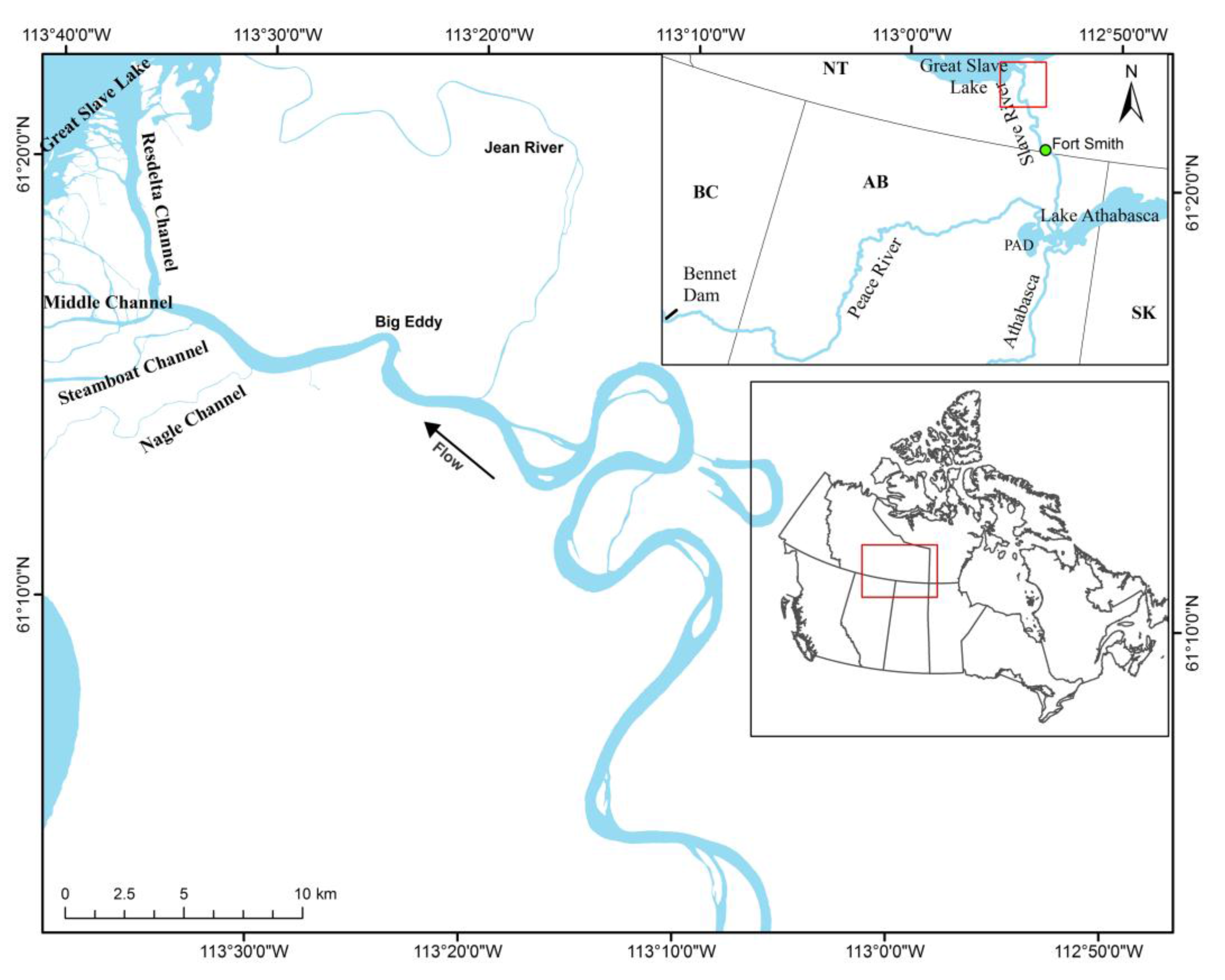
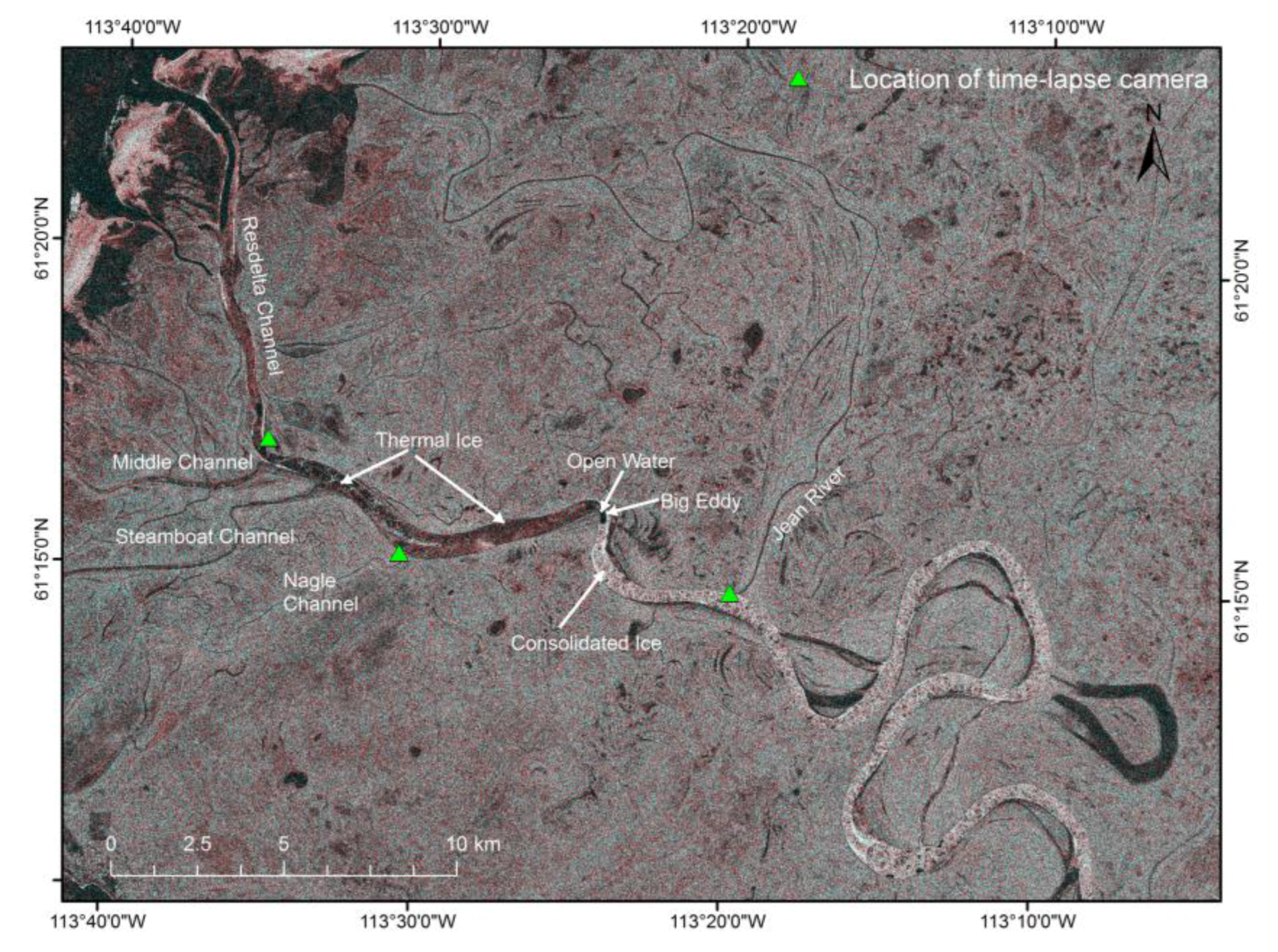
2.1. Study Area

The Slave River (Figure 1) is a large transboundary river in Canada, flowing as a continuation of the Peace River in Alberta and emptying into Great Slave Lake in the Northwest Territories (NWT). It draws from a huge watershed that includes the Peace River, Athabasca River, Lake Athabasca, and the Lower Slave River sub-basins, and extends across parts of the NWT and the provinces of Alberta, British Columbia, and Saskatchewan, with a drainage area of 616,400 km2. The Slave River contributes approximately 75% of the inflow to Great Slave Lake, with a mean annual flow of 3400 m3/s, and carries an average of 30 million tonnes of suspended sediment into Great Slave Lake each year [21]. Due to the development of oil, gas and hydroelectric production in the upstream portion of the Slave River watershed over the last several decades, concerns have been raised regarding the river’s water quality, ice cover regime, and ecosystem health, all of which are important for the traditional lifestyle of its communities. The Slave River Delta is located on the southeastern side of Great Slave Lake, covers an area of approximately 640 km2 and consists of several active channels including the Resdelta (main channel), Middle, Steamboat, and Nagle channels (Figure 1).
Figure 1. Study area in the Slave River Delta. The study area was zoomed in the red color box.
Remotesensing 07 13664 g001

2.2. Space-Borne Radar Data and River Ice Monitoring

Space-borne synthetic aperture radar (SAR) systems measure and record the amount of microwave energy that is scattered from the target in the direction of the sensor; this is defined as radar backscatter. The strength of the backscattered signal from the target is highly dependent on the electrical properties, the structure of the surface and subsurface layers (e.g., surface roughness, thickness of layers) and incident angle. Detailed descriptions on how microwaves interact with freshwater ice and SAR characteristics can be found in Weber et al. [10], Nghiem and Leshkevich [22], and Unterschultz et al. [13]. Regarding the electrical properties of water-ice layers, the parameter quantifying the electrical properties of any given layer, relative to those of free space, is known as the relative dielectric constant (Ɛr). This parameter of river ice and snow is almost entirely dependent on the absence of water and it also determines the absorption and scattering loss of the electromagnetic waves from snow/ice layers. An ice layer with higher dielectric constant and higher water and moisture content, produces higher signal return compared with that of the layers with low dielectric constant, such as clear and dry snow/ice layers. If the absorption loss is high, the penetration depth of the microwave signal is low and, thus, the recorded backscatter largely reflects the properties of surface layers (e.g., snow) rather than the underlying ice [10,13]. For example, an ice layer comprised of wet snow with as little as 5% free water, significantly reduces the penetration of microwaves to 10 cm in depth at 5 GHz frequency [23]. The dielectric constant of clear and dry ice of freshwater ranges from 2.0 to 3.2; that is, a low-loss medium [24,25,26]. In such ice layers, the microwave signal with the frequency from 1 to 10 GHz can penetrate to depths ranging from 100 m to 10 m, respectively. As a result, the appearance of a given ice layer in radar images differs significantly in wet conditions, as compared to dry conditions [10].
In the observation of river ice, the backscatter energy is governed by the interaction of microwaves with four components—water, ice, snow, and air—through two general mechanisms: surface and volume scattering. Surface scattering involves the reflection of microwaves at the interface with target components, while volume scattered radar signals penetrate the surface and then are scattered due to impurities within the ice volume. Surface scattering is often observed in either specular or diffuse reflection, depending on surface roughness. Specular reflection often occurs from smooth surfaces (e.g., water surface, or an ice cover with water on the surface), reflecting significant amounts of incident microwave energy away from the sensor (forward scattering), and hence show up relatively dark on a radar image. Diffuse scattering occurs on rough and wet ice surfaces, and the incident signal is reflected nearly uniformly in all directions [10,13]. Depending on the incidence angle of SAR systems, the proportion of the incident energy in diffuse scattering directed back toward the sensor will be different. For example, in RADARSAT-2 satellite images acquired with incident angles from 20 to 50 degrees, rougher ice surfaces result in higher backscatter amounts received by the sensor and appear relatively brighter in the image [13]. As such, when classifying river ice covers it is sometimes challenging to separate ice surfaces from areas of rapids or under high current and wind conditions along a given river. In volume scattering, the return signals depend not only on radar system parameters, such as wavelength, polarization, and incident angle, but also on the structure and the heterogeneity of the imaged object. Similar to diffuse surface scattering, volume scattering contributes significant amounts of radar backscatter and is positively related to the degree of discontinuity of ice volume such as cracks, air inclusions (or air bubbles), water pockets, and impurities [8,13]. In radar imagery, highly heterogeneous ice covers (e.g., juxtaposed and consolidated ice covers) can be expected to have higher radar return signals from both surface and volume scattering and appear brighter in the image.
Regarding the SAR sensor characteristics, such as wavelength, polarization, incidence angle, and viewing geometry, observations of river ice types and structures also strongly depend on these parameters. For example, analysis of the two co- (e.g., HH—horizontal transmit and horizontal receive) and cross- (e.g., HV—horizontal transmit and vertical receive) polarizations can reveal different information about the ice cover characteristics. The HH-backscatter signals have a good correlation with ice thickness, while HV return signals correlate better with fresh snow depth [18]. Additionally, depending on the polarization and ice cover types, the radar backscatter returned from freshwater ice covers is significantly influenced by the incidence angle of the system [22]. In co-polarizations (i.e., HH and VV), the radar backscatter has a negative relationship with incidence angle over a range from 20 to 60 degrees. For example, the ice class consisting of crushed and broken plates of ice and snow ice with 3–5 cm of snow yields the highest backscatter values at all incident angles. Backscatter of pancake ice is high at small incidence angles (i.e., less than 30 degrees) and then significant decreases to a low value of a new ice layer at 60 degrees. New freshwater ice often has the lowest backscatter among the different ice types because it contains almost no air bubbles or other volume scatterers. With the very smooth surface and no ice cover, calm open water has the lowest backscatter values at all incidence angles [22]. These patterns of backscatter values are different in the images of co-polarized backscatter ratio (e.g., r = VV/HH). The new freshwater ice, consolidated ice, and open calm water have positive correlations with incidence angles. The backscatter of pancake ice increases with the incidence angle ranging from 20 to 30 degrees, while it decreases when the incidence angles increases from 30 to 60 degrees [22]. These properties of different ice types observed at different incidence angles and polarizations have important implications for the selection of radar beam modes when monitoring changes in river ice covers.
In this study, RADARSAT-2 SAR single-look complex (SLC) data were used for automatic monitoring of river ice freeze-up and progression in the Slave River Delta. RADARSAT-2 operates in a sun-synchronous, dawn-dusk orbit using C-band imaging frequency (5.405 GHz or 5.55 cm wavelength). At this frequency, the microwaves can potentially penetrate through the entire ice thickness on Canadian rivers, and thus the data are suitable for river-ice monitoring of the Slave River Delta. Two single beam modes, wide fine mode (FOW3) and wide fine quad polarization mode (FQ17W), were used in this study (Table 1). Images from the FOW3 product have a nominal ground swath of 150 km and a nominal resolution of 5.2 × 7.7 m. The FOW3 covers the incident angle range from 38.7 to 45.3 degrees [27]. The FOW3 product, with dual co- and cross-polarizations of HH and HV, was used to classify river-ice types in the two winter seasons from 2013 to 2015 in the Slave River Delta channel, and to analyze variations in the ice cover during winter 2014. Since we did not have enough FOW3 images in winter 2015 for the calculation of ice cover variance, the FQ17W images were used to analyze the variation in the ice cover during winter 2015 (Table 1). The FQ17W mode offers full polarizations (HH+VV+HV+VH) at a smaller swath of approximately 50 km, covering any area from 35.7 to 38.6 incidence angle degree. The nominal resolution of FQ17W images is 5.2 × 7.6 m [27]. As the calculation of ice cover variation for the two winter seasons was conducted separately with two radar datasets (FOW3 and FQ17W), and the results of variance were normalized to be comparable (see Section 2.4), the use of two different RADARSAT-2 beam modes with different incidence angles was not expected to influence the interpretation of ice cover variation during the two winter seasons.
Table 1. RADARSAT-2 data for monitoring freeze-up and ice cover progression during winter 2014 and winter 2015 in the Slave River Delta.
IDAcquired DatePolarizationBeam ModeIncidence AngleStudy Purpose
121 November 2013HH+HVFOW338.7–45.3To classify ice cover types and analyze ice cover variation during winter 2014
215 December 2013HH+HVFOW338.7–45.3
38 January 2014HH+HVFOW338.7–45.3
41 February 2014HH+HVFOW338.7–45.3
525 February 2014HH+HVFOW338.7–45.3
610 December 2014HH+HVFOW338.7–45.3To classify ice-cover types during winter 2015 and compare with winter 2014
73 January 2015HH+HVFOW338.7–45.3
819 December 2014HH+HV+VH+VVFQ17W35.7–38.6To analyze ice cover variation during winter 2015 and compare with the variation in winter 2014
912 January 2015HH+HV+VH+VVFQ17W35.7–38.6
105 February 2015HH+HV+VH+VVFQ17W35.7–38.6
111 March 2015HH+HV+VH+VVFQ17W35.7–38.6

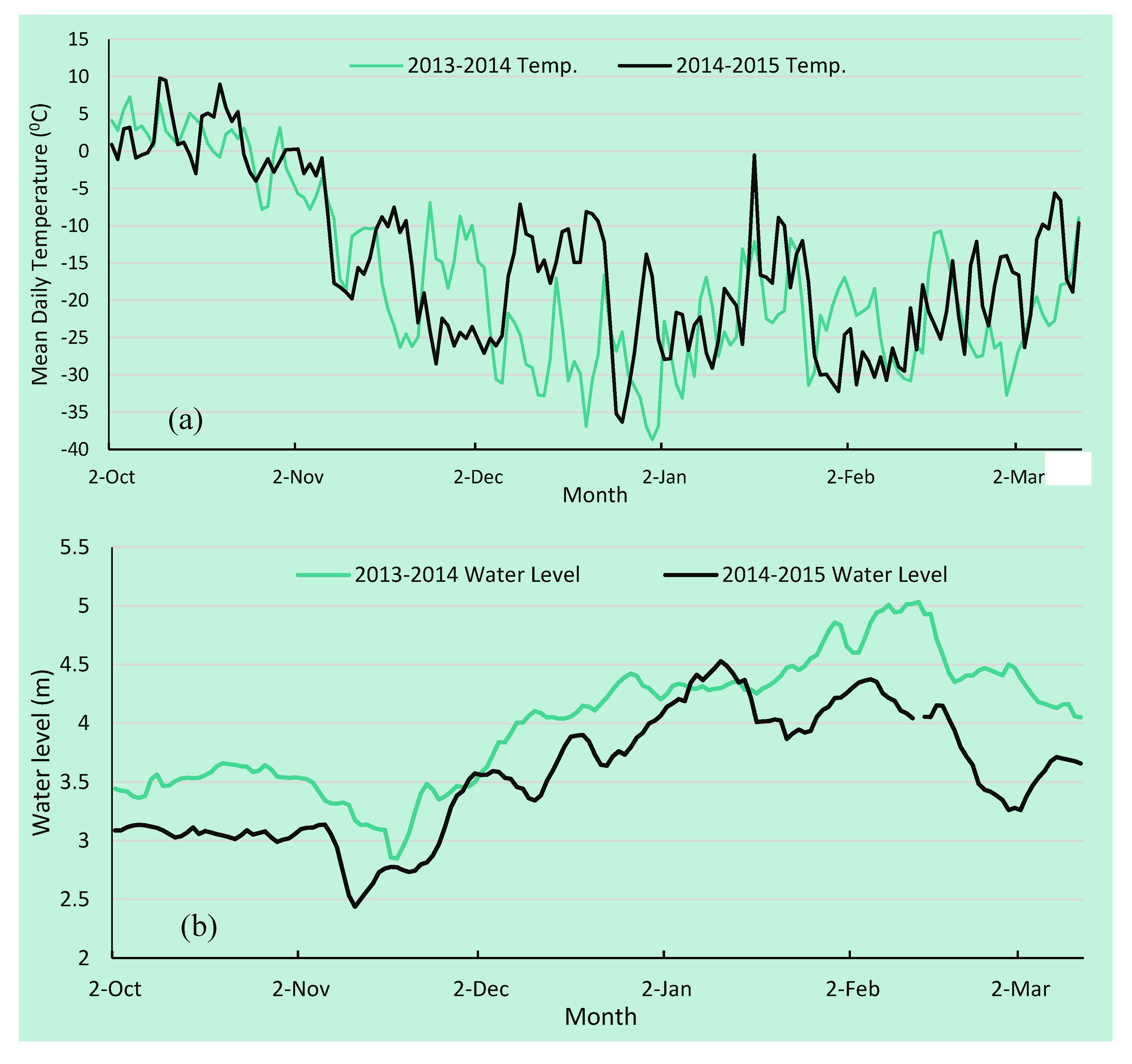
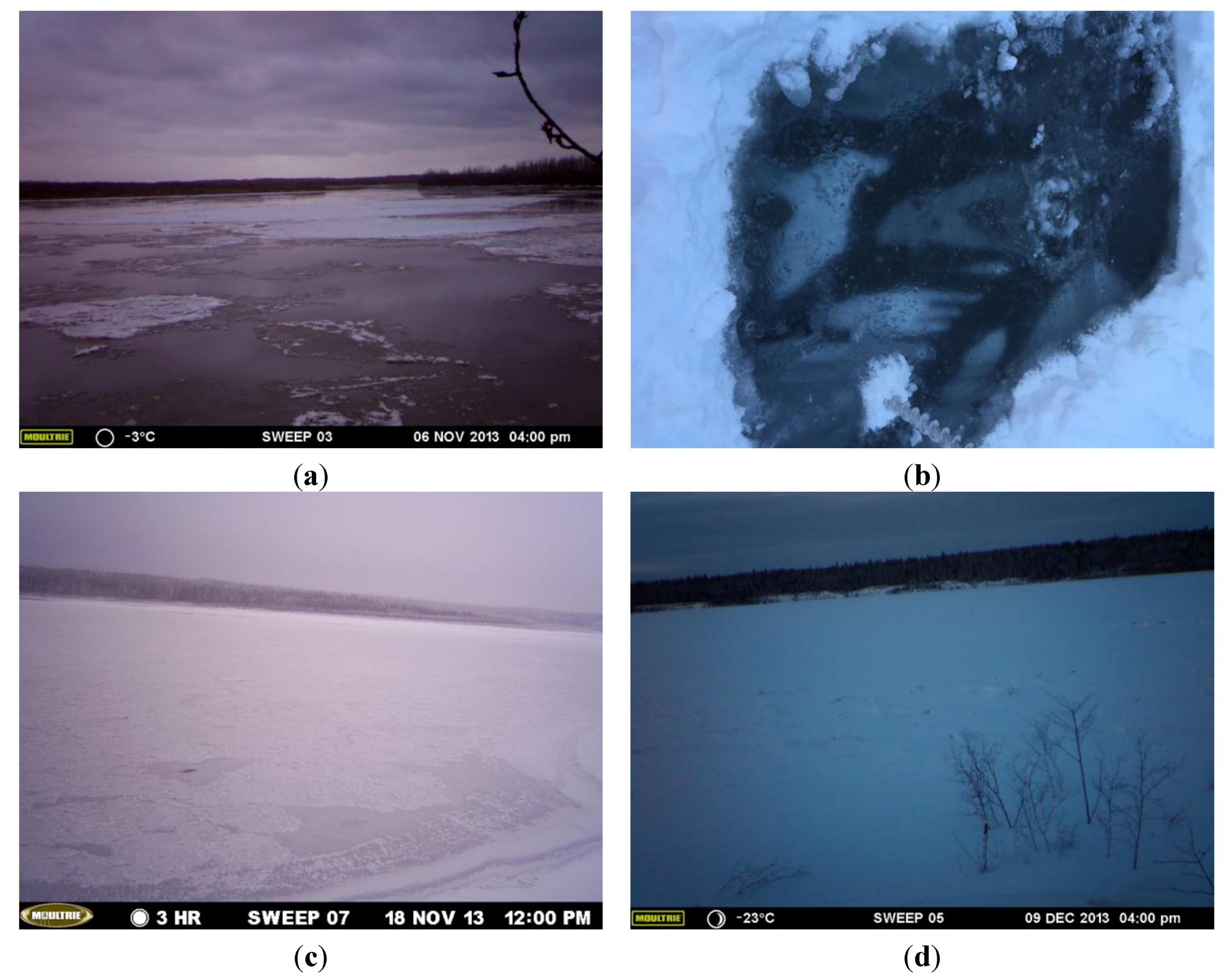
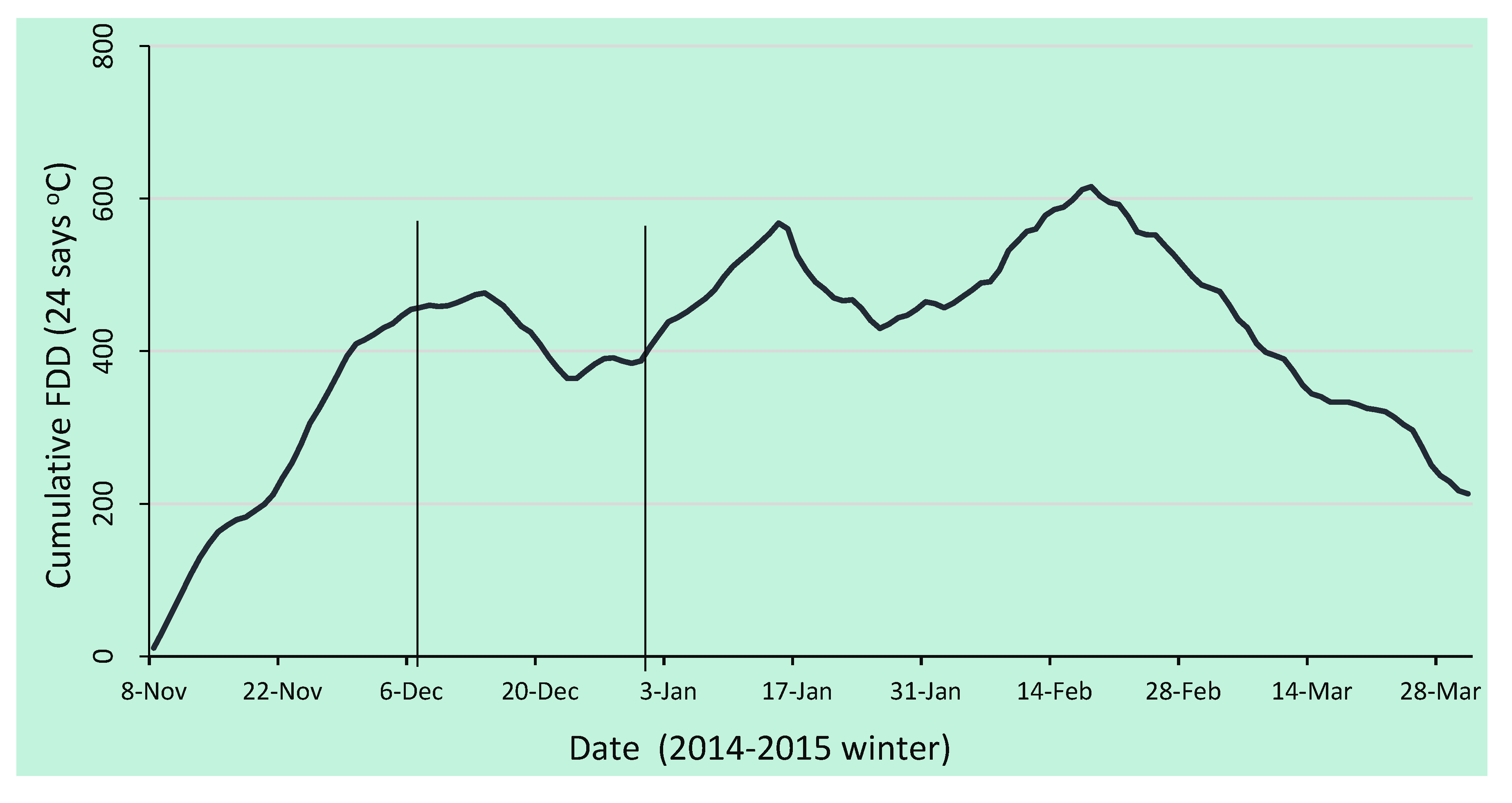
2.3. Characteristics of the Slave River Freeze-Up

The characteristics of river ice freeze-up and progression in the Slave River Delta have been documented by Das et al. [6], but a brief summary of these results is warranted here to help with the interpretation of the satellite imagery in the present study. The ice regime of the river depends on the meteorological, hydraulic, and geomorphologic conditions (e.g., air temperature, discharge, water level, and river slope) of the river. Since air temperature decreases dramatically at the end of October and early November (Figure 2) along the Slave River, frazil ice typically forms during the second week of November when air temperatures are consistently below 0 °C and the river flow has receded [6]. While the air temperature and discharge continue to decrease, frazil ice particles adhere to each other to form ice floes. These floes may then be arrested due to the constriction of the river, forming juxtaposed ice [4,6]. After ice floes and juxtaposed ice accumulate at an ice bridging section to form a stable ice cover, thermal ice growth from the cover’s underside in the vertical direction occurs to produce a black or thermal ice layer. Frazil ice from upstream can also be deposited under an existing ice cover along the river throughout the winter. Due to the relatively low river bed slope and low turbulence at the delta portion of the river, a juxtaposed ice cover begins at the Slave River Delta and then extends upstream to Fort Smith (Figure 1). Water pockets and air bubbles are also formed, particularly at the upstream portion of the Delta along the stretch between Big Eddy and the Nagle Channel.
Figure 2. Daily air temperature (a) and water level (b) during the winters 2013–2014 and 2014–2015 recorded at Fort Smith and Fitzgerald—upstream of Slave River Delta—respectively.
Remotesensing 07 13664 g002
The heterogeneity of the ice structure, ice thickening and deposition of frazil ice underneath the ice cover resulted in a large amount of backscatter upstream from Big Eddy, showing brighter color on the radar image (Figure 3). This ice cover sheet is interpreted as a consolidated ice cover, extended in the upstream direction. In the lower portion of the Slave River channel, downstream from Big Eddy to the river mouth at Great Slave Lake, three classes—open water, thermal ice, and juxtaposed ice covers—can be identified on the November RADARSAT-2 image, showing an increase in backscatter values in these three classes (Figure 3). More specifically, the low backscattering between Big Eddy and Nagle Channel reveals the persistence of a “white” ice layer. Similarly, the stretch between Nagle Channel and Steamboat Channel was dominated by thermal “black” ice cover which was observed in the field. Generally speaking, four classes—open water, thermal ice, juxtaposed ice, and consolidated ice—are dominant along the Slave River between November and March. It should be noted that the occurrence of these types of ice covers along the river depends on climatic, hydraulic and geomorphologic conditions, as well as the timing of ice monitoring. For example, in the December 2013 and January 2014 images, most of the river sections at the Slave River Delta were ice covered with three dominant classes: thermal, juxtaposed, and consolidated ice. Therefore, the analysis of multi-temporal RADARSAT-2 data is expected to automatically identify different ice covers, as well as their progression during the freeze-up period along the Slave River. Figure 4 shows different ice types along the Slave River from Fort Smith to Great Slave Lake on the time-lapse photos that can be matched to the ice types in the radar images.
Figure 3. Example of ice cover types identified visually on sigma-nought RADARSAT-2 imagery (FOW3 beam mode), acquired on 21 November 2013. The HH, HV, and HV polarizations were assigned the colors red, green, and blue, respectively, for the image display. (RADARSAT-2 Data and Products © MacDonald, Dettwiler and Associates Ltd. (2013)—All Rights Reserved. RADARSAT is an official trademark of the Canadian Space Agency).
Remotesensing 07 13664 g003
Figure 4. The formation of different ice types along the Slave River from Fort Smith to Great Slave Lake (a) including frazil pans or ice floes; (b) thermal ice; (c) juxtaposed ice, and (d) consolidated ice. The time-lapse photos were taken near the Jean River in the delta channel (a) and Bell Rock Landing in Fort Smith, upstream of the delta channel (c and d). The ground photo (b) shows the thermal ice layer with snow coverage, taken in Fort Smith during the field survey on 24 January 2015. As there is no available RADARSAT-2 images in early November, the frazil ice and ice floes (a) were not identified in this study.
Remotesensing 07 13664 g004

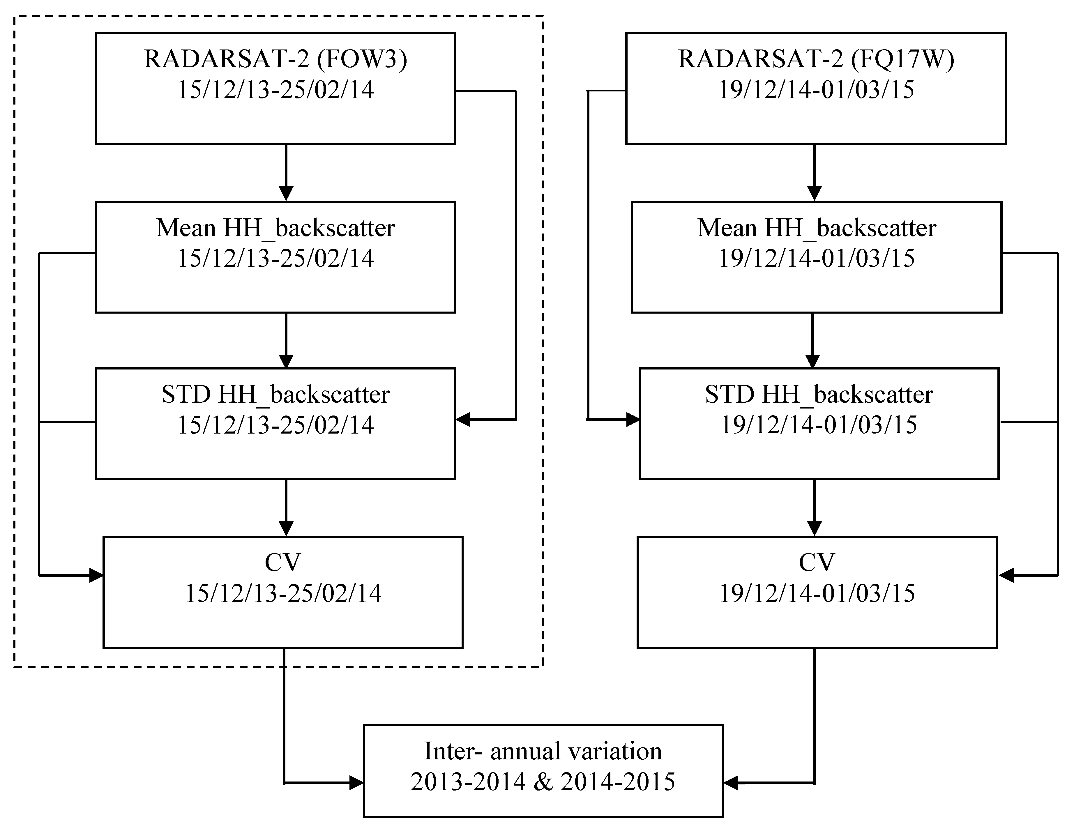
2.4. Radar Backscatter Based River Ice Variation

Multi-temporal RADARSAT-2 data (FOW3 and FQ17W beam modes) during the 2013–2015 winters (Table 1) were received as single look complex (SLC) magnitude values for each slant range pixel. As interpolation into ground range coordinates is not performed during processing for SLC image products, the initial step orthorectified all downloaded images to the UTM NAD 83 coordinate system, with a pixel size of 10 × 10 m. During this process of image ingestion, radiometric calibration was conducted to convert SLC data to power values, where power equals the radar backscatter. The lookup tables (LUTs) provided with the SLC data were used to apply a fixed offset and a range-dependent gain function to the data to generate the calibrated image (i.e., sigma-nought). The sigma-nought images were then interpreted as the power (or intensity) of radar backscatters for further analysis. The Kuan and median filtering approaches were applied to decrease speckle noise and to increase the effective number of looks in the data. The adaptive Kuan and median filters with a 5 × 5 kernel size, that reduce speckle while preserving the sharp contrast variation (edges) [28], were used in our study.
The intra-annual and inter-annual variation and dynamics of the ice covers in the 2013–2014 and 2014–2015 winters were assessed and compared using the backscatter based coefficient of variation (CV) along the river transect. The CV represents the ratio of the standard deviation to the mean indicating the variability of a series of numbers, independent of the unit of measurement used [29,30]. The method is a useful statistic for comparing the degree of variation of different data series even if their mean are different from each other. As the backscatter values contain information of river ice formation and its structure, the variation of backscatter in the radar images represents the changes of river ice cover. In addition to the standardization of the CV, the independent calculation of the CV in the 2013–2014 and 2014–2015 winters, using FOW3 and FQ17W products, respectively, will not affect the interpretation and comparability of river ice variation between the two winter seasons. The CV (CVice_cover) was calculated by using mean (MEANHH_backscatter) and standard deviation (STDHH_backscatter) of HH-backscatter values for each pixel, over the freeze-up period in the Slave River Delta (November to March) (Equation (1)). As the HH-backscatter signals have been cited as an indicator of ice thickness [18], the use of HH-backscatter in the CV calculation has implications for the dynamics of the river-ice cover as well as river-ice thickness in the Slave River Delta channel.
CVice_cover = STDHH_backscatter/MEANHH_backscatter
where:
MEAN HH _ backscatter = i = 1 n HH i / n
STD HH _ backscatter = 1 n ( HH MEAN HH backscatter ) 2 / ( n 1 )
n—Number of input RADARSAT-2 images; HHi—co-polarization HH backscatter of image number i, after filtering speckle.
In this study, the CVice_cover was calculated twice for the 2013–2014 winter to assess intra-annual variation of ice covers. The first CVice_cover was calculated with five FOW3 input images, acquired from 21 November 2013 to 25 February 2014. Four FOW3 input images, acquired from 15 December 2013 to 25 February 2014, were used for the second CVice_cover (Figure 5). Since there were only four FQ17W images acquired during the 2014–2015 winter, with a similar acquisition time to the last FOW3 image in the previous winter (Table 1), the second CVice_cover profile in the 2013–2014 winter was used to compare the ice cover variation of the 2014–2015 winter (Figure 5) in an inter-annual assessment.

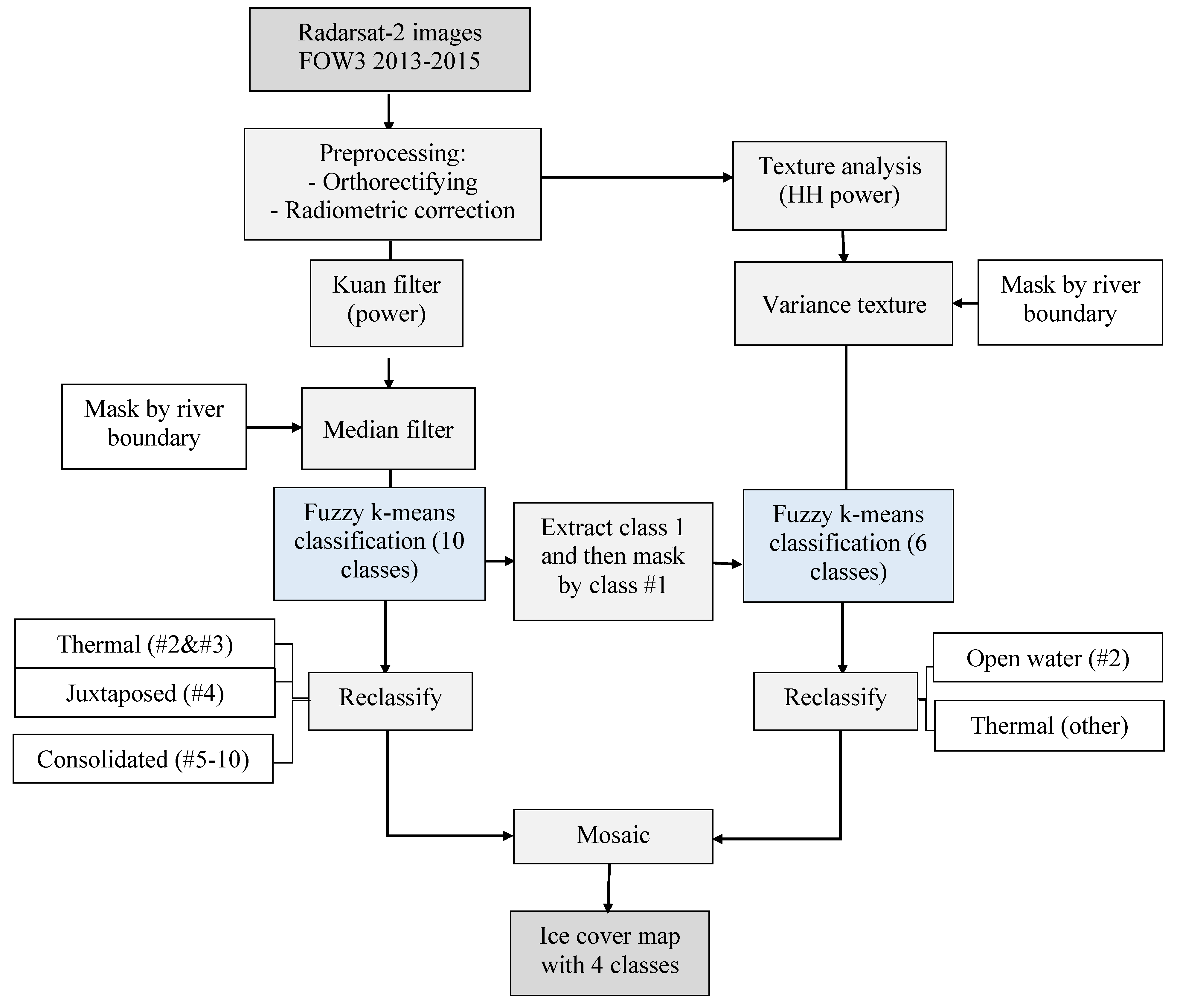
2.5. Mapping Algorithm of River Ice Types

In addition to using the Kuan and median approaches to decrease speckle noise, the calibrated power radar data were also analyzed for texture, prior to applying the unsupervised fuzzy k-means classifier in mapping breakup ice types. The de-speckle step is to enhance the classification of homogeneous pixels, while the texture analysis is to characterize the structural heterogeneity and micro patterns of classes. Therefore, the inclusion of texture analysis in the mapping algorithm was expected to discriminate smooth to moderately rough ice covers, e.g., open water and thermal “black” ice covers on radar images, associated with low texture and low backscatter. In contrast, the backscatter-based classification applied to filtered images is more efficient in discriminating ice cover types with high backscatter, such as juxtaposed and consolidated ice [11]. In the texture analysis, the grey level co-occurrence matrix (GLCM) [31] was applied to derive texture properties of homogeneity, contrast, dissimilarity, mean, variance, and entropy. All these texture properties were examined to select the optimal texture for the classification of ice covers in this study. Even though the GLCM mean appeared to be the most efficient in reducing speckle on radar images, it is more suitable for classifying large features (e.g., consolidated ice), which can be identified using backscatter-based classification of filtered images. Other texture properties including homogeneity, contrast, dissimilarity and entropy, had a very “grainy” appearance and provided little information for discriminating different ice covers. Since the purpose of using texture-based classification in this study was to separate open water from thermal “black” ice cover, the variance-texture based classification showed the optimal result and thus was selected.
Figure 5. Analyzing the process of spatio-temporal variation in the ice cover in the 2013–2014 and 2014–2015 winters. A similar process of CV calculation (dash box) was applied to RADARSAT-2 (FOW3) images acquired from November 2013 to February 2014, to monitor intra-annual variation of ice cover of the 2013–2014 winter (13 November–14 February).
Remotesensing 07 13664 g005
In the next step, the unsupervised fuzzy k-means method was applied to both backscatter-filtered and texture-analyzed images. The unsupervised fuzzy k-means classifier was the most common clustering method used in a number of studies that mapped ice cover in Canadian rivers (e.g., [7,10,11,12,16]. The aim of the fuzzy k-means approach is data reduction, to aid in information transfer in the field of pattern recognition [32,33,34]. Data reduction is conducted by translating a multiple attribute description of an object into k membership values, with respect to k classes which represent the fuzzy behaviour. For further details on the fuzzy k-means algorithm, readers are refer to Sulaiman et al. [33], Dehariya et al. [32], and Jain [34]. In general, the fuzzy k-means classifier uses an iterative procedure that starts with an initial random allocation of the objects to be classified into k clusters. Given the cluster allocation, the centre of each cluster is calculated as the weighted average of the attributes of the objects. In the next step, objects are reallocated among the classes according to the relative similarity between objects and clusters based on distance analysis (e.g., Euclidian, diagonal, or Mahalanobis). Reallocation continues by iteration until a stable result is reached, in which similar objects with similar reflectance (or backscatter) characteristics are grouped together in each cluster. The advantage of k-means clustering, as well as other unsupervised methods is that they require no prior training data. Therefore, it is suitable for application to remotely sensed data for remote regions, such as high northern latitudes, where collection of training samples is difficult due to accessibility. In the first stage of the ice mapping algorithm, the fuzzy k-means was used on the backscatter-filtered images to create 10 classes. We examined a different number of backscatter classes as inputs in the classifier to select the optimal number of classes with respect to the separation of ice classes with slight differences in backscatter values, such as open water and thermal ice, juxtaposed ice and consolidated ice. The assignment of different backscatter classes to the ice cover types (i.e., consolidated ice, juxtaposed ice, thermal ice, and open water) was based on the responses of river ice covers to radar signals (see Section 2.2 and Section 2.3) and visual interpretation of ice cover types along the Slave River in the image acquired on 21 November 2013 [6]. The first class (#1), with the lowest backscatter, was then extracted to create a mask on the texture-analyzed images for classifying open water and thermal ice. The backscatter classes from #2 to #10 (low to high backscatter values) were reclassified to create thermal ice (#2 and #3), juxtaposed ice (#4), and consolidated ice (#5 to #10). In the second stage of ice mapping, the fuzzy k-means classifier was applied to the texture-analyzed images to identify six classes of ice cover types. Only pixels (classes) within the mask from class #1, the first stage of backscatter-based classification, were extracted. These classes were then reclassified to create open water and thermal ice layers. Subsequently, three classes of thermal, juxtaposed and consolidated ice from the first classifying step were mosaicked with two classes of open water and thermal ice from the second step, creating the final ice cover map for the Slave River. Only those imagery information were extracted that coincided with the polygon areas of the river sections which are available from the CanVec database at Natural Resources Canada. Additionally, both co- (HH) and cross- (HV) polarizations were used in the backscatter-based classification of filtered images, while the texture-based classification was used with a single co-polarization (HH) backscatter. The mapping algorithm was primarily developed based on the ice cover conditions on the 21 November 2013 RADARSAT-2 image and then applied to all other images from both studied winters (Table 1). In order to compare the thresholds of backscatter values corresponding to different ice types, the backscatter samples (in dB unit) of each ice type were also extracted. The classification and regression tree method [35] was then applied on these samples to derive the backscatter thresholds. The PCI Geomatica 2014 was used to process all images, including the unsupervised classification of images based on the fuzzy k-means algorithm. The overall processing flow for mapping the ice cover is shown in Figure 6.
Figure 6. Processing steps for mapping river ice in Slave River from RADARSAT-2 data.
Remotesensing 07 13664 g006

2.6. Validation

The results from the automated ice-cover classification were compared with the visual image analysis (e.g., see [6]), the time-lapse camera imagery collected during the winter 2013–2014 and the meteorological and hydraulic conditions (i.e., daily air temperature and water discharge) in the two studied winters. This study used a Moultrie D-333 seven megapixel waterproof outdoor camera with different photo capture modes including time lapse, hybrid, and motion detection, to collect field photos of ice cover progression in the Slave River Delta. There were three time-lapse cameras installed near the inflows to the Jean River, Nagle Channel and Middle Channel, from December 2013 to March 2014 (Figure 3). All cameras were mounted on trees and were programmed to take three pictures per day. The meteorological and hydraulic conditions were obtained from Environment Canada’s weather station at Fort Smith and the real-time gauging station on the Slave River at Fitzgerald, operated by the Water Survey of Canada (Figure 2).

3. Results and Discussion

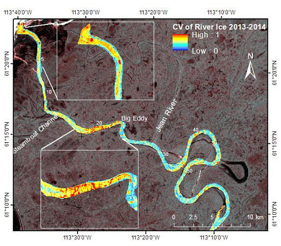
3.1. Spatio-Temporal Variation of the Ice Cover along the Slave River Delta Channel

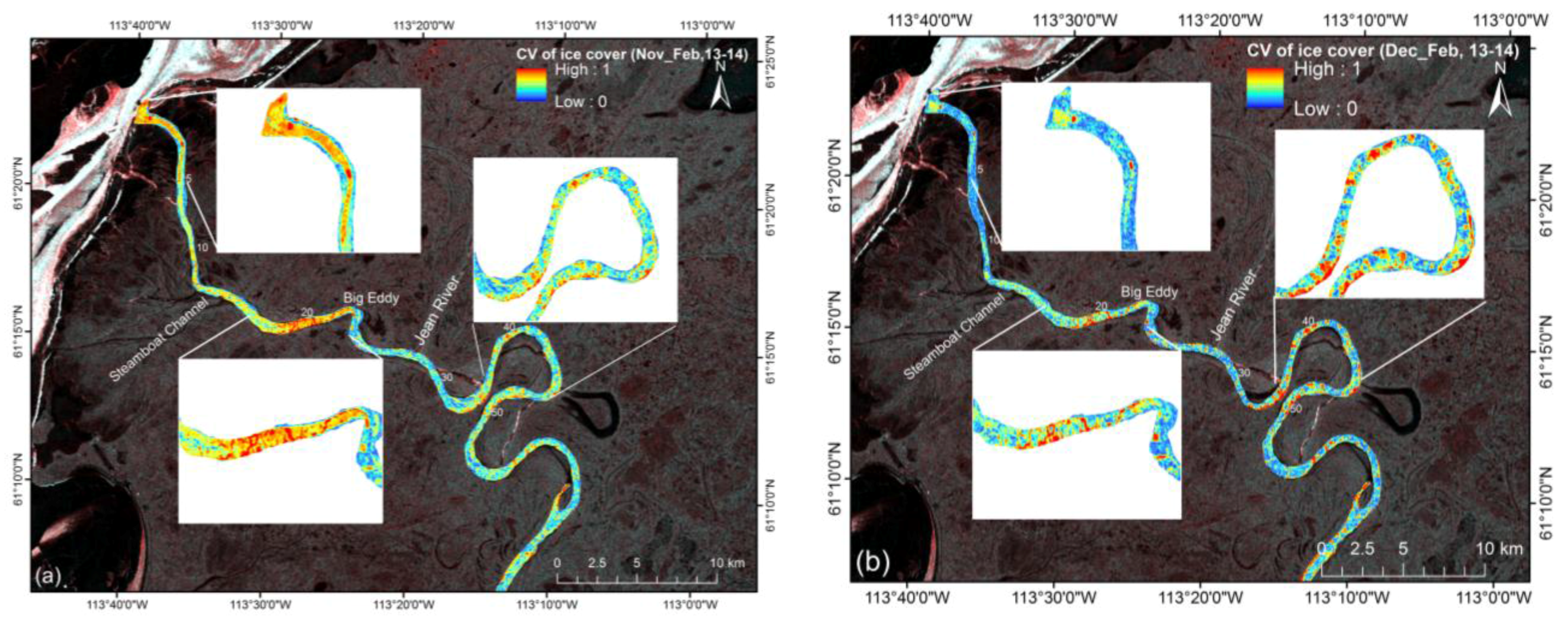
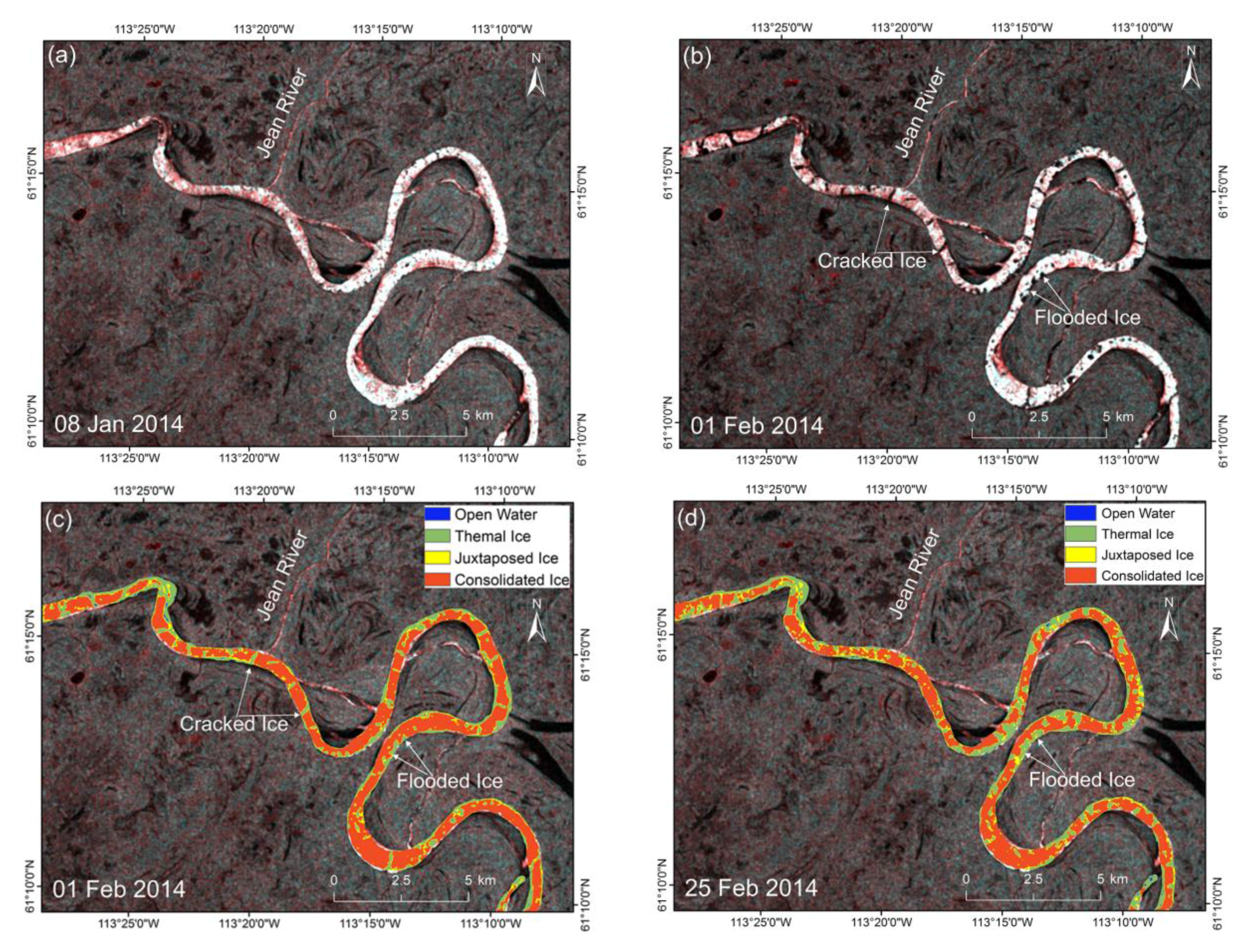
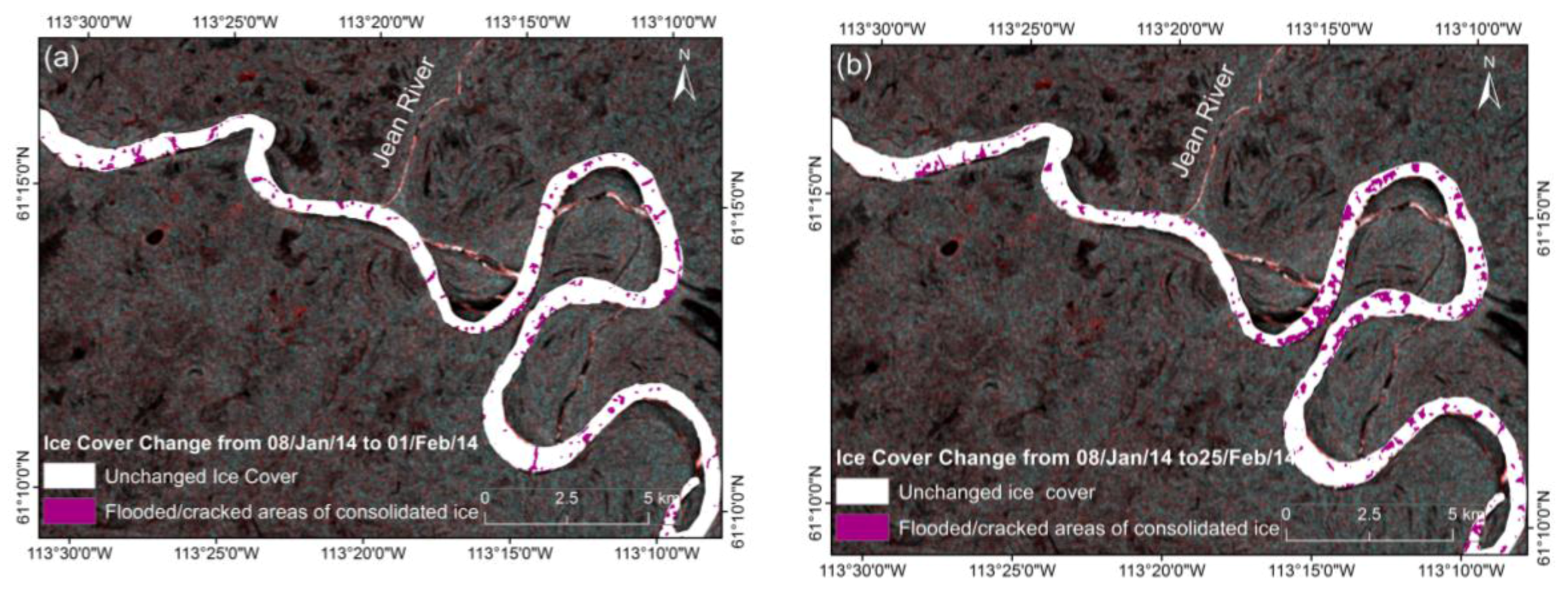
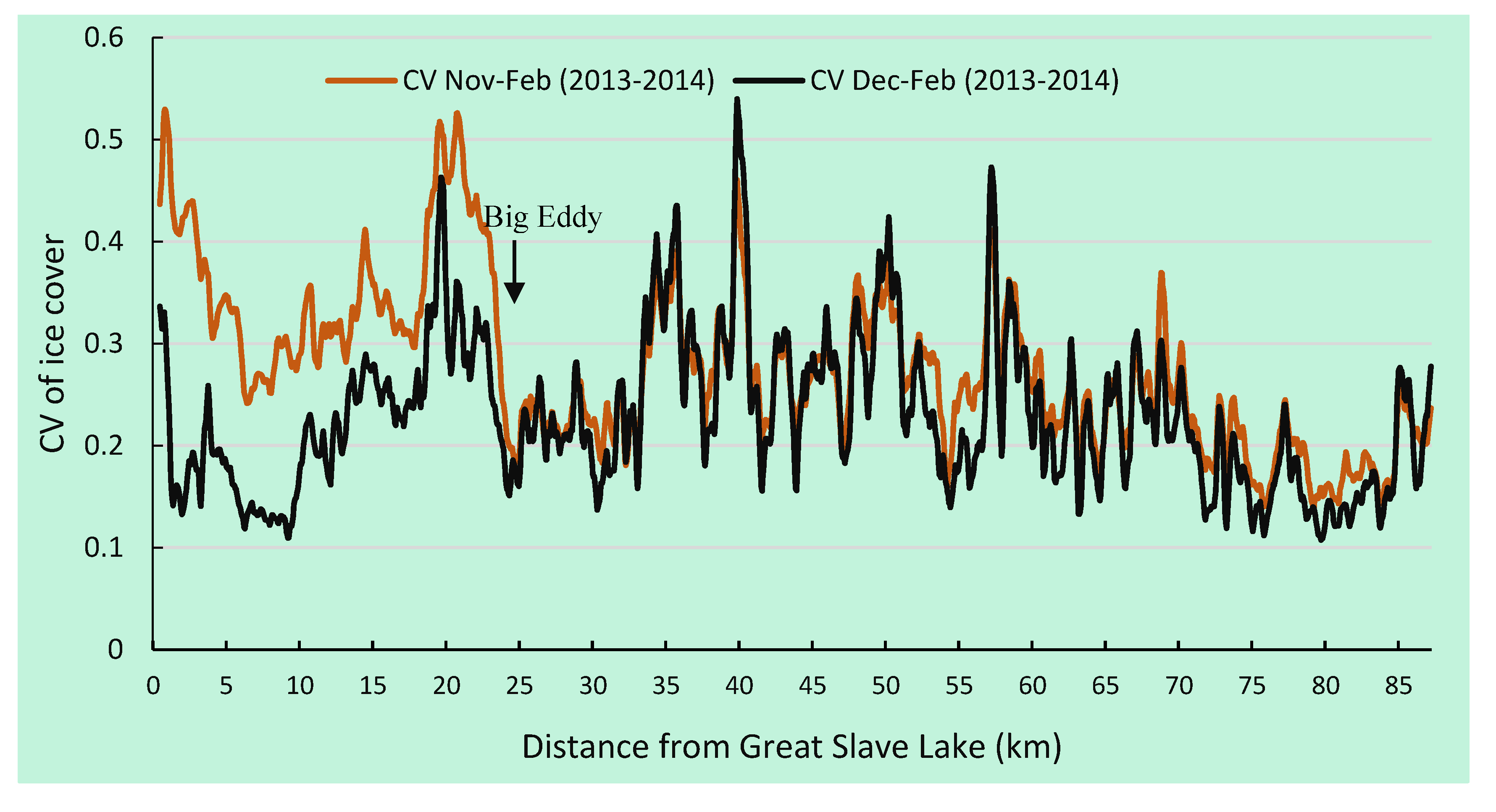
3.1.1. Intra-Annual Variation of the Ice Cover

In the intra-annual assessment of river ice covers, a high variation was observed in the river sections from Big Eddy to Nagle Channel and in Resdelta Channel near Great Slave Lake (Figure 7 and Figure 8).The similar pattern in river ice variation between November-February and December-February periods in the sections upstream of Big Eddy reveals more stable ice cover conditions than the downstream sections, starting from the last week of November (Figure 8). In addition to the influence of Great Slave Lake, the drastic decrease in air temperature starting in early November 2013 and the increase in water level from November 2013 to February 2014 (Figure 2) contributed to the formation of different ice-cover classes, which ranged from dominant thermal ice in November 2013 to consolidated ice in January and February 2014 in the downstream river sections. Additionally, the high variation in the ice cover from Big Eddy to Great Slave Lake might indicate the deposition of frazil ice in this downstream river section. Since ice bridging occurred at Big Eddy in the first week of November 2013, due to the narrower and sinuous nature of the river, ice floes were arrested at that point to form a juxtaposed ice cover and then a consolidated ice cover extending upstream from the bridging (i.e., at Big Eddy). As a result, more stable conditions in the ice cover from the last week of November, extending upstream from Big Eddy, were observed in the 2013–2014 winter. The intra-annual variation in the ice cover in the 2013–2014 winter has implications for the processes of ice-cover formation that reflect the spatio-temporal influence of different geomorphological, hydraulic, and climatic characteristics along the river.
Figure 7. Intra-annual variation of ice covers along the Slave River Delta channel during the 2013–2014 winter, from November to February (a) and from December to February (b). The number along the river (e.g., 5, 10, etc.) indicates the kilometer distance from the river mouth at Great Slave Lake. (RADARSAT-2 Data and Products © MacDonald, Dettwiler and Associates Ltd. (2013–2014)—All Rights Reserved. RADARSAT is an official trademark of the Canadian Space Agency).
Remotesensing 07 13664 g007
Figure 8. Profiles of backscatter-based coefficient of variation showing an intra-annual variation of ice covers along the Slave River Delta channel during the 2013–2014 winter.
Remotesensing 07 13664 g008

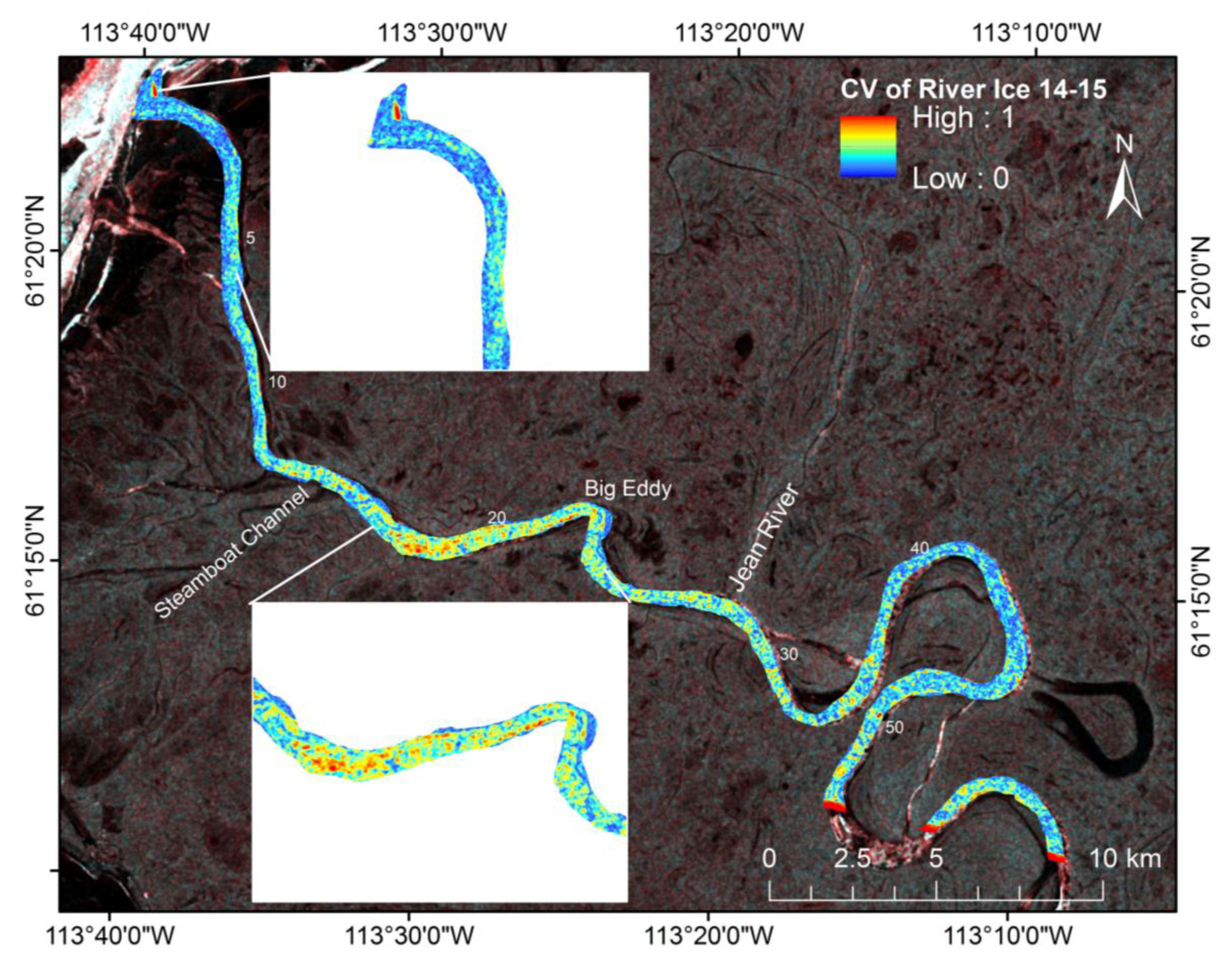
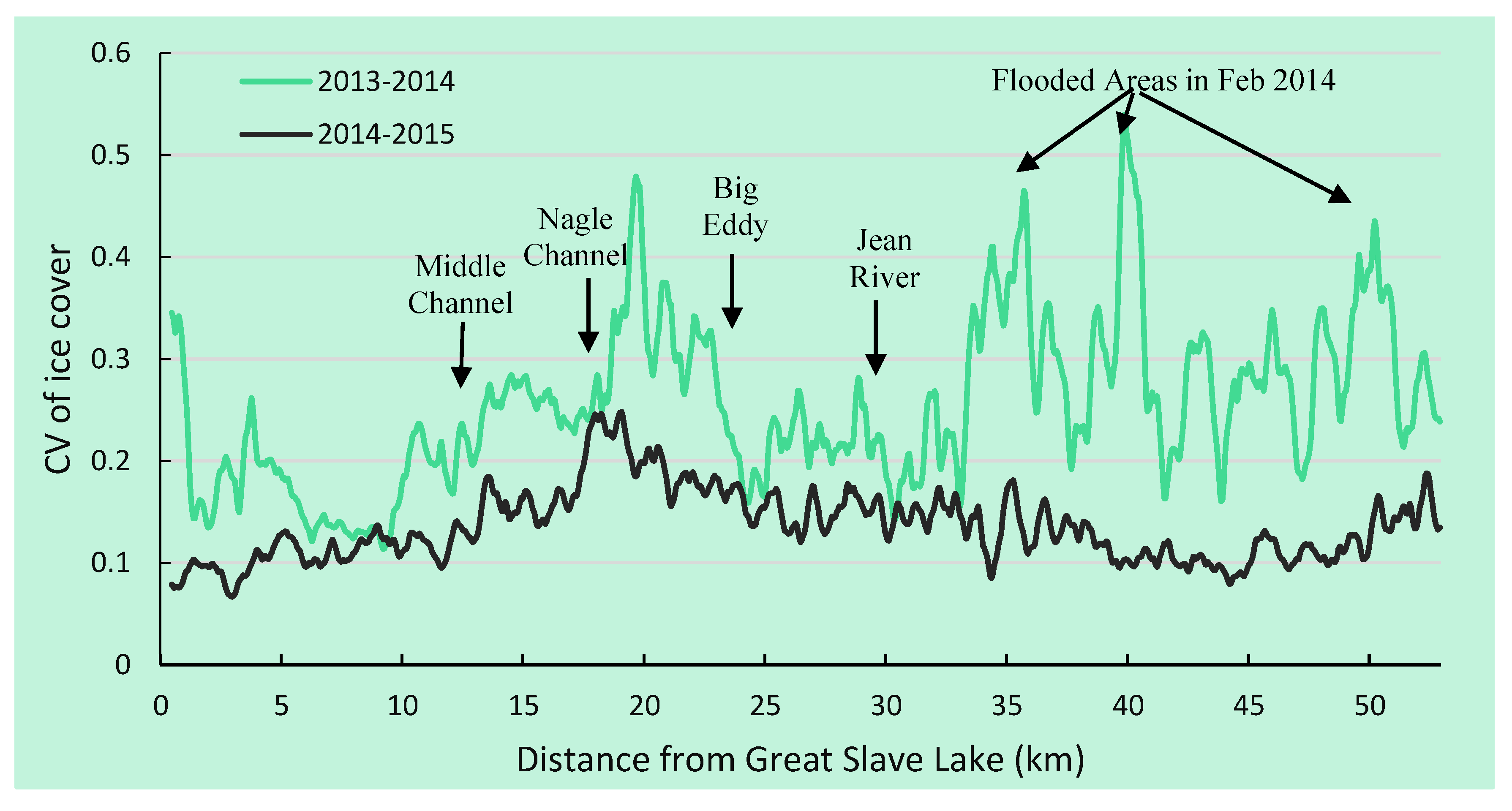
3.1.2. Inter-Annual Variation of the Ice Cover

For the purpose of comparison of river-ice variation between the 2013–2014 winter and the 2014–2015 winter, only RADARSAT-2 images from December to February were used to derive CVice_cover for both winters (Figure 7b and Figure 9). The extracted profile of CVice_cover along the river sections (Figure 10) showed that the variation in ice cover in the 2013–2014 winter was much higher than the variation in the 2014–2015 winter. In general, the higher variation of air temperature and water level defined the higher variation of ice covers in the 2013–2014 winter compared with that of the 2014–2015 winter (Figure 9). More specifically, the standard deviation of air temperature in the 2013–2014 winter was higher than the 2014–2015 winter, 0.85 and 0.80 respectively. The dramatic increase in water level from mid-December 2013 to the middle of February 2014 exerted higher forces on the ice cover, compared to the subsequent winter, may define the high variation in the ice cover along the river in the 2013–2014 winter. Between mid-December and mid-January of both winters, there was a similar pattern of water level increase. By the first week of February 2014, stage increased drastically to 5 m and remained high until mid-February 2014, while the stage increase in February 2015 was lower at around 4.2 m (Figure 2b). An increase in the water level increases the water pressure on the ice cover resulting in cracking and dislodgement of the ice cover from the banks and subsequent flooding of the cover. As a result, the high variation in the ice cover along the river can be observed in the 2013–2014 winter. However, it should be noted that the patterns of ice-cover variation could change if there were changes in the timing of observations, as well as the number of input RADARSAT-2 images, e.g., extending the assessment period from October to March, as there were temporal changes in meteorological and hydrological conditions (Figure 2). In addition, the spatial variation in the ice cover can also be explained by geomorphological characteristics along the river and Great Slave Lake. As such, the cracked/flooded areas in February 2014 seemed to occur in narrower and more sinuous sections, showing high variation in the ice cover, i.e., approximately 30 km to 50 km upstream of the Slave River Delta channel (Figure 7b and Figure 10).
Figure 9. Variation in ice cover along the Slave River Delta channel from December to February in the winter 2014–2015. The number along the river (e.g., 5, 10, etc.) indicates the kilometer distance from the river mouth at Great Slave Lake. (RADARSAT-2 Data and Products © MacDonald, Dettwiler and Associates Ltd (2013–2015)—All Rights Reserved. RADARSAT is an official trademark of the Canadian Space Agency).
Remotesensing 07 13664 g009
Figure 10. Inter-annual variation in ice cover along the Slave River Delta channel during the freeze-up period (mid-December to end-February) in the winters 2013–2014 and 2014–2015.
Remotesensing 07 13664 g010

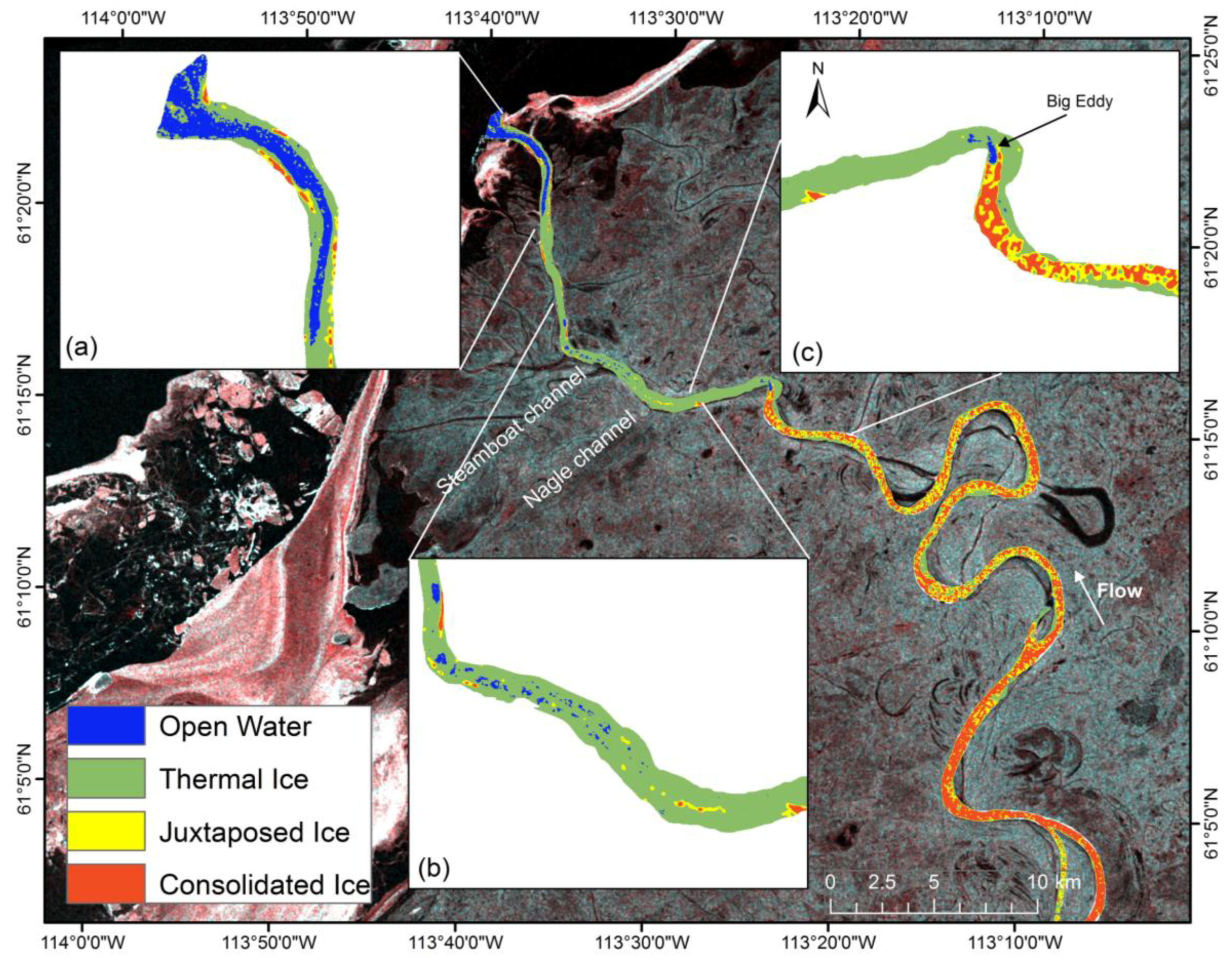
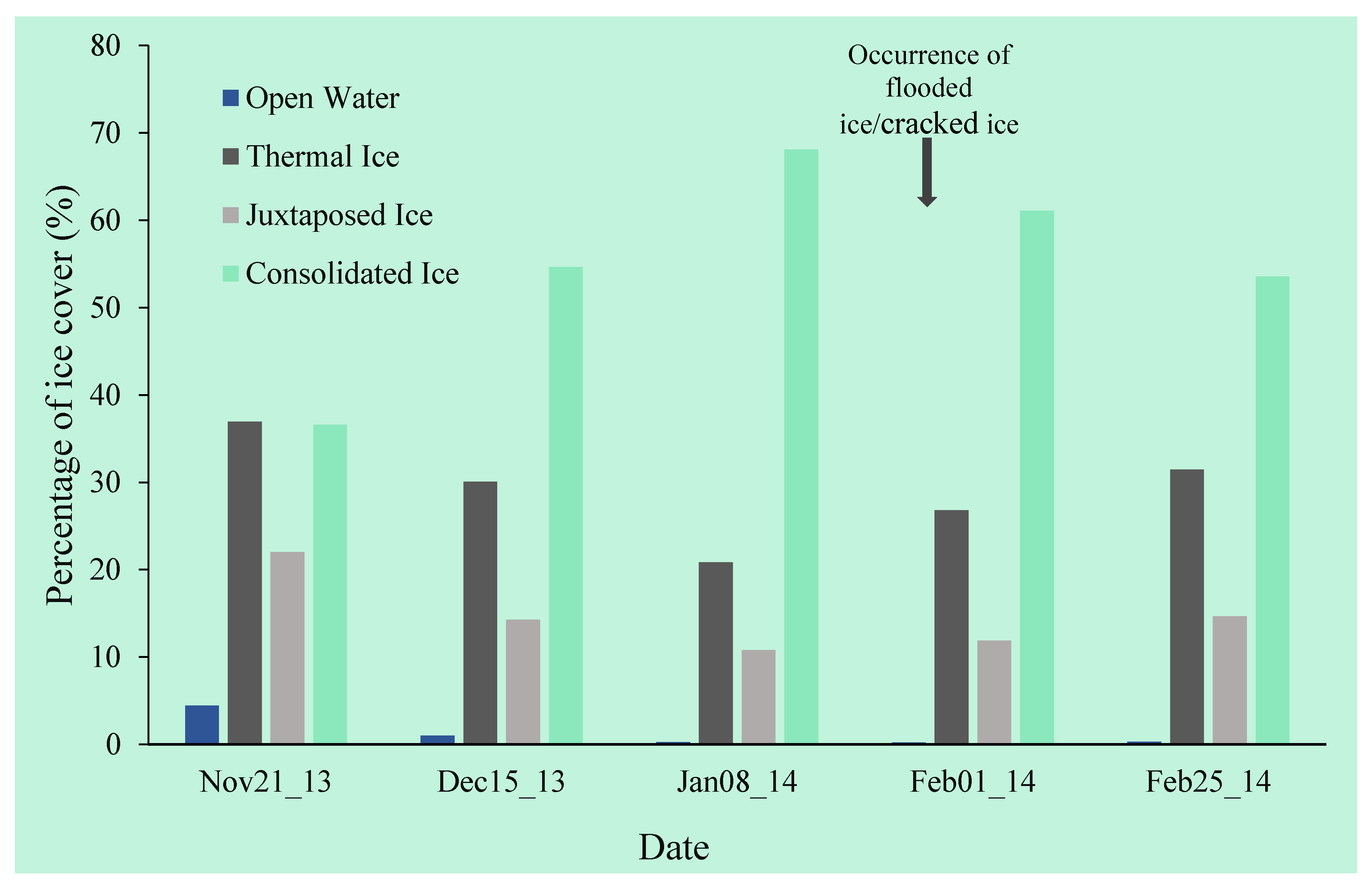
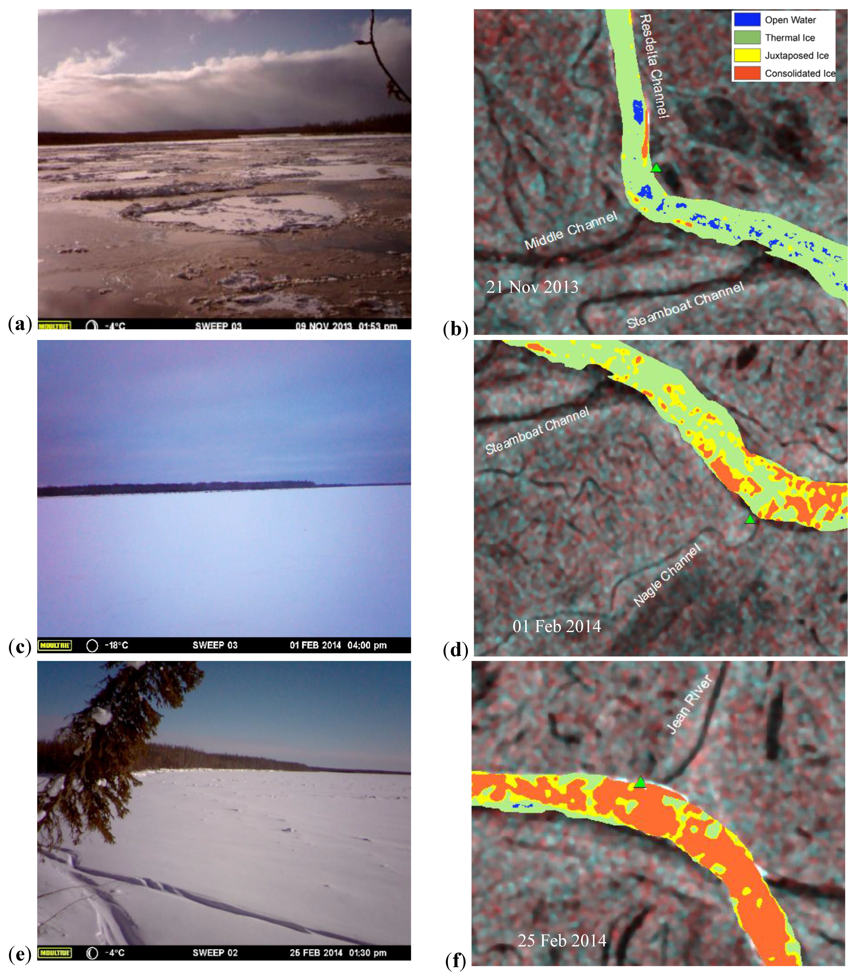
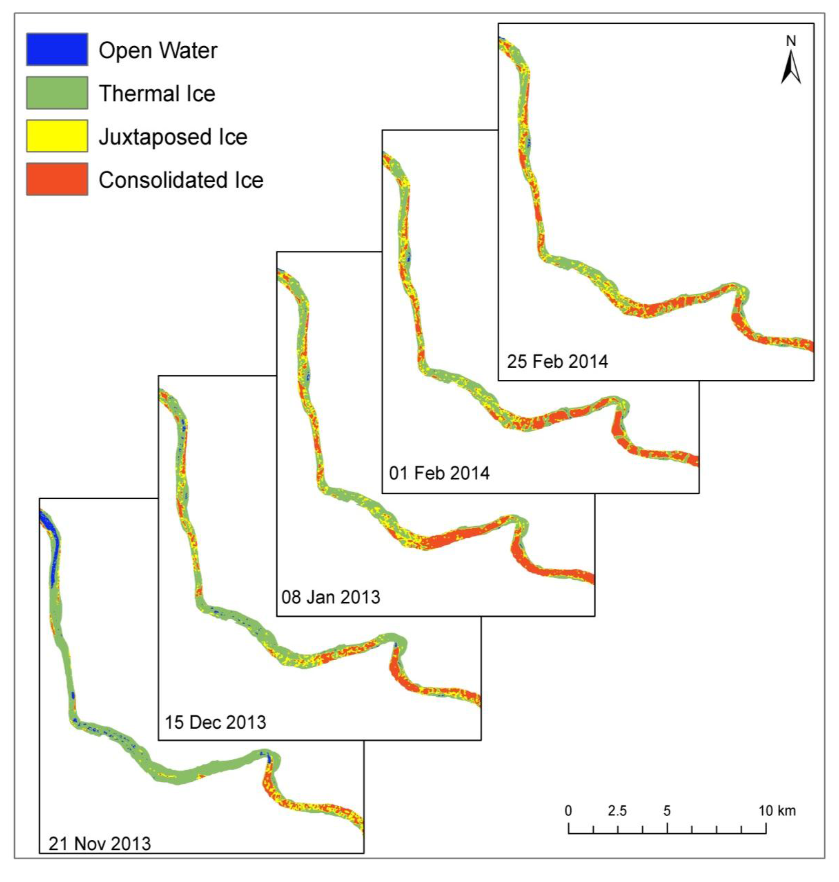
3.2. Monitoring Ice Cover Types and Freeze-Up Progression during Winter 2013–2014

The results of the unsupervised classification of river-ice covers from 21 November 2013 RADARSAT-2 images are shown in Figure 11. Almost all of the Slave River Delta channels were ice covered, except for portions of the river in the Resdelta Channel and Big Eddy. In the Resdelta Channel, border ice progressed from both shorelines of the river toward the middle of the channel (Figure 11a). The river section from Big Eddy to the Resdelta Channel was mainly covered by thermal ice (Figure 11b,c). During this time, ice bridging also occurred at Big Eddy which caused the flow of ice to be arrested and juxtaposed ice to form and, subsequently, the formation of consolidated ice that extended in the upstream direction. In order to compare the variation of different ice types in association with radar backscatter, the extraction of backscatter values corresponding to each ice type was also conducted. The thresholds of backscatter values showed that the consolidated ice leads to the highest backscatter values (>−8 dB), while open water results in the lowest backscatter values (<−18 dB). Backscatter values ranging from −18 dB to −11 dB and from −11 dB to −8 dB indicate thermal ice and juxtaposed ice layers, respectively.
Figure 11. Ice cover on 21 November 2013 in the Slave River Delta channel, (a) ice cover in Resdelta Channel, (b) ice cover between Nagle Channel and Resdelta Channel, (c) ice cover between Jean River and Nagle Channel (RADARSAT-2 Data and Products © MacDonald, Dettwiler and Associates Ltd. (2013)—All Rights Reserved. RADARSAT is an official trademark of the Canadian Space Agency).
Remotesensing 07 13664 g011
The time-lapse photos taken during the freeze-up period in the 2013–2014 winter showed consistent patterns of ice-cover classification from the RADARSAT-2 imagery (Figure 12). There is no available clear time-lapse photos in the last two weeks of November 2013 to compare with the classified image on 21 November 2013. The photo taken on 9 November 2013 at the Resdelta Channel showed the progress of the freezing-up, with frazil ice adhering and forming ice floes and then juxtaposed ice. Additionally, ice floes from upstream also traveled downstream along the river (Figure 12a), unless they were arrested at an ice bridging section or a river constriction. With the temperature steadily decreasing and the downstream river sections being typically wider and less steep than the upstream reach, those ice covers thermally thickened to form black or thermal ice layers. Subsequently, the classified images from November to February (Figure 13) showed dominant coverage with thermal ice, from Big Eddy to Great Slave Lake. From the middle of December to the end of February, juxtaposed and consolidated ice gradually formed downstream from Big Eddy (Figure 12c,d and Figure 13), particularly between the middle of December and middle of January, since the lowest temperature (Figure 2a) was observed during this period in the 2013–2014 winter. This facilitated the extension of border ice, causing ice floes along the river to accumulate edge to edge on the water surface to form juxtaposed, and then consolidated, ice. As a result, the proportion of consolidated ice cover increased from November 2013 to January 2014, coinciding with a decrease in other ice types (Figure 13 and Figure 14). However, a significant increase in the upstream water level in February 2014 (Figure 2b) caused the ice cover to form cracks or to dislodge from the river banks due to the high stresses, allowing water to reach the top of the ice surface and flooding large sections of the ice cover, particularly in mid-February. Due to the forward scattering of microwaves off of the water surfaces, lower backscatters in these flooded or cracked areas returned to the sensor and hence, these areas are classified as thermal ice or juxtaposed ice, leading to a decrease in the consolidated ice cover in February and an increase in thermal ice (Figure 14 and Figure 15). This may be a misclassification of the mapping algorithm, since some of the consolidated ice sheet was actually covered by water. However, it is noteworthy to mention that a new layer of thermal ice can also form in the cracked or flooded areas, since the temperature is still below 0 °C.
In comparison with the backscatter based river ice variation, the ice cover maps show consistent patterns with the intra-annual variation of ice cover along the delta channel in the 2013–2014 winter (Figure 8 and Figure 13). The changes between different ice cover types that lead to high CVice_cover, were observed in the downstream portion of the channel as well as in the possible flooded/cracked ice covers upstream from Big Eddy.
In order to eliminate the cracked/flooded areas possibly caused by an increase in water level and water discharge, the ice-cover map from 8 January 2014 was used to analyze the difference from the ice cover maps from February 2014. More specifically, the ice-cover map layer from 8 January 2014 was subtracted from the map layers from 1 February 2014 and 25 February 2014. The results showed that almost all cracked/flooded areas were changed from consolidated ice cover and connected to the shore (Figure 16), with the cracked/flooded areas increasing from 5.6% to 11% of total ice cover between 1 February and 25 February 2014. Since the ice layer along the shore may be thinner than in the middle channel, an increase in the upstream water level and discharge might result in the dislodgement of these ice layers from the shore and then extend to the ice layer in the middle of channel. Further observations of this phenomenon are necessary to confirm whether the ice layer is cracked or covered by water. This has important implications for ice and water management along the Slave River when there is an increase in the water level.
Figure 12. River ice covers from time-lapse camera (left) and remotely-sensed data (right), (a) & (b)—ice cover between Steamboat Channel and Resdelta Channel, (c) & (d)—ice cover between Nagel Channel and Steamboat Channel, (e) & (f)—ice cover near Jean River. Location of time-lapse camera is shown in blue triangle. (RADARSAT-2 Data and Products © MacDonald, Dettwiler and Associates Ltd. (2013–2014)—All Rights Reserved. RADARSAT is an official trademark of the Canadian Space Agency).
Remotesensing 07 13664 g012
Figure 13. Freeze-up progression along the Slave River Delta channel from Jean River to Great Slave Lake.
Remotesensing 07 13664 g013
Figure 14. Percentage of ice cover along the Slave River Delta channel in winter 2013–2014.
Remotesensing 07 13664 g014
Figure 15. Occurrence of flooded/cracked areas along the Slave River Delta channel during winter 2013–2014. RADARSAT-2 images without and with flooded/cracked areas of ice cover acquired on 08 January 2014 (a) and 1 February 2014 (b), respectively, and classification of ice covers on 1 February 2014 (c) and 25 February 2014 (d) images, identifying an increase in flooded areas as misclassification with thermal ice cover. (RADARSAT-2 Data and Products © MacDonald, Dettwiler and Associates Ltd. (2014)—All Rights Reserved. RADARSAT is an official trademark of the Canadian Space Agency).
Remotesensing 07 13664 g015
Figure 16. Flooded/cracked areas of ice cover on 1 February 2014 (a) and 25 February 2014 (b). (RADARSAT-2 Data and Products © MacDonald, Dettwiler and Associates Ltd. (2014)—All Rights Reserved. RADARSAT is an official trademark of the Canadian Space Agency).
Remotesensing 07 13664 g016

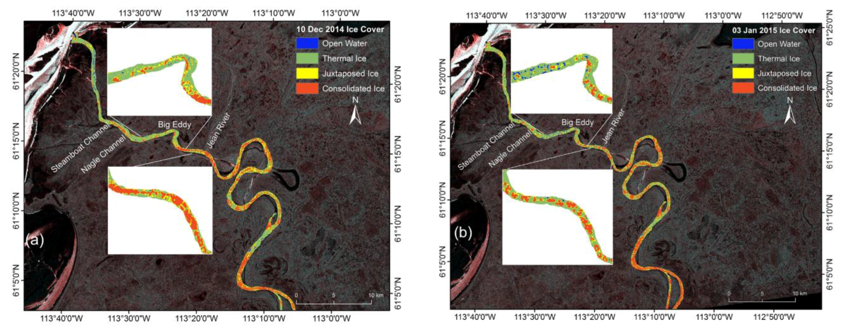
3.3. Monitoring the Ice Cover during Winter 2014–2015

The mapping algorithm for the 2013–2014 winter was used to derive the ice cover for the winter 2014–2015 from RADARSAT-2 imagery (FOW3 beam mode). Similar to the 2013–2014 winter, thermal ice was of the dominant ice cover type from Big Eddy to Great Slave Lake during the 2014–2015 winter (Figure 17). The dominance of thermal ice in the downstream portion of the river in the 2014–2015 winter was confirmed by our field survey in late January and early February 2015 from Big Eddy to the Steamboat Channel. All drilled ice holes, using an auger, showed the dominance of thermal ice type along the river sections from Big Eddy to the Steamboat Channel (Figure 18).
From December 2014 (Figure 17a) to January 2015 (Figure 17b), there was a decrease in the consolidated ice cover along the Slave River Delta channel, particularly in the river section from Jean River to Big Eddy. Since the repeat cycle of the RADARSAT-2 satellite is 24 days, observations recorded by the satellite can account for some characteristics as well as progressions of river ice dynamics within 24-day cycles. The 24-day accumulation of freezing day degrees (FDD) showed that the cumulative FDD on 10 December 2014 was higher than that of 3 January 2015 (Figure 19). This could explain the changes in the ice cover between December 2014 and January 2015. Additionally, the higher water level in the period between 10 December 2014 to 3 January 2015, compared to the period from 25 November and 10 December 2014, upstream of Fitzgerald, 3.8 and 3.4 m, respectively, could put stresses on the ice cover. As a result, an increase in thermal ice and open water cover in the 3 January 2015 image (Figure 17b) may indicate some flooded/cracked areas along the delta channel, due to a peak of water level and mean air temperature in the second week of January 2015 (Figure 2a,b). This pattern of ice cover might be similar to that observed in February, 2014 (Figure 15 and Figure 16). Unfortunately, we did not have the same FOW3 beam mode imagery from RADARSAT-2 to confirm flooded areas as there were in the 2013–2014 winter.
Figure 17. Ice cover during winter 2014–2015, from RADARSAT-2 images acquired on 10 December 2014 (a) and 3 January 2015 (b). (RADARSAT-2 Data and Products © MacDonald, Dettwiler and Associates Ltd. (2014–2015)—All Rights Reserved. RADARSAT is an official trademark of the Canadian Space Agency).
Remotesensing 07 13664 g017
Figure 18. Thermal ice samples between Big Eddy and Nagle Channel (a) and between Nagle Channel and Steamboat Channel (b), collected during the field survey on 30 January 2015.
Remotesensing 07 13664 g018
Figure 19. Cumulative freezing degree days (FDD) recorded at Fort Smith during the freeze-up period in winter 2015. The two vertical lines indicate the dates (i.e., 10 December and 3 January) of the acquired RADARSAT images in the 2014–2015 winter as shown in Figure 12 (data source: Environment Canada 2015).
Remotesensing 07 13664 g019

4. Conclusions

Using remote sensing approaches, the intra-annual and inter-annual spatio-temporal patterns of ice formation and variation along the Slave River Delta channel were analyzed. The RADARSAT-2 backscatter-based CV analysis was first introduced in this study, providing insights into river ice cover variations with time effectively. The river sections with high variations during the course of winter may indicate weak spots along the ice cover, which has important implications for river ice management and the safety of public travel along the river. Even though the thickness of different ice covers was not calibrated in this study, our previous studies of other river systems (e.g., [18]) showed that HH RADARSAT-2 backscatter has a positive correlation with river ice thickness. This might reveal that the high variation in HH backscatter measured by the CV analysis indicates the fluctuation in ice thickness possibly implying reductions in ice strength along the river sections. The high variations in ice cover are due to the changes in hydraulic, meteorological, and geomorphic conditions along the river as well as the influences of Great Slave Lake at the river mouth. Further analysis of river ice variations with higher temporal resolution of radar data and an association with driving factors will assist to quantitatively explain the variations of ice cover and predicting river ice-induced natural hazards, such as ice cracking and ice jam flooding.
In our mapping algorithm of river ice types, the combination of two classification procedures, backscatter-based and texture-based fuzzy k-means classifications, effectively delineated four major river-ice and water classes (open water, thermal ice, juxtaposed ice, and consolidated ice) along the Slave River Delta channel during the freeze-up period from November to March of two winters. Even though we did not have enough field samples for a quantitative validation of river-ice maps, the results were compatible with our findings from field observations and visual interpretations of the RADARSAT-2 imagery, as well as geomorphological, hydraulic, and meteorological characteristics of the river delta channel. Similar to studies of the Peace River [7,10,11,12], Saint-Francois River [12,17] and Koksoak River [16] in Canada, the texture analysis was useful for discriminating classes with slight differences in roughness and backscatter values, i.e., open water and thermal ice layers. Similarly, the backscatter-based classification of filtered images could easily identify ice cover types with high backscatter signals, such as juxtaposed and consolidated ice. The field observation in the 2014–2015 winter indicated the dominance of thermal ice in the river reach between Big Eddy and Great Slave Lake, showing consistent patterns with ice cover maps. Even though the radar system has the ability to penetrate snow and, thus, reflect structure and properties of river ice cover, the dependence of relative dielectric constants of river ice and snow on water content influence the penetration depth of radar backscatter. Wet snow covers can reduce penetration depth dramatically resulting in the large recorded backscatter returned from the snow layer rather than the underlying ice [13,23]. As a result, the identification of river ice types using radar backscatter might have biases if there are occurrences of wet snow covers on ice layers. Similarly, due to the influences of environmental conditions (e.g., changes in air temperature and flow conditions), the structure or thickness of one ice type may vary that lead to possible dynamics of radar backscatter in different time periods. Therefore, further studies are necessary to account for the influences of snow cover as well as other environmental conditions on mapping accuracy of river ice types using radar images. Additionally, there are some concerns about the influence of the noise floor on radar imagery that might limit the separation of new ice and open water [36,37], particularly when using RADARSAT-2 ScanSAR and Quad Polarization beam modes and/or cross-polarization channels (i.e., HV or VH) [38,39]. In addition to the correction for interchannel crosstalk in the RADARSAT-2 satellite [38,40], using wide fine imaging beam mode (FOW3) and the HH polarization channel in this study can reduce the influence of the noise floor on the classification of different ice types and open water. However, the impact of the noise floor on the mapping algorithm in this study requires further investigation to precisely quantify the error of ice maps.
Since the ice regime can change spatio-temporally, due to variability in flows and different meteorological and geomorphological conditions, the continuous monitoring of river-ice dynamics along the river, as well as year to year changes is necessary to fully understand the Slave River system and its interaction with other ecosystems and natural hazards. Further research using remote sensing, with additional field data and a longer monitoring timeframe, is imperative to confirm our findings related to the river’s ice cover behaviour, strength, and characteristics for both freezing-up and breakup periods. The continuous research also helps to build an historical database of ice cover conditions for the future management.

Acknowledgments

We thank the Canada Excellence Research Chair (CERC) at the Global Institute for Water Security (GIWS), the Canadian Water Network (CWN), and Slave Watershed Environment Effect Program (SWEEP) for funding this research. We are also grateful for the Canadian Space Agency’s (CSA) support by supplying radar images through their Scientific Operational Applications Research—Education (SOAR-E) program and the C-CORE led project Water Ecosystems Monitoring using Earth Observation (WAMEO).

Author Contributions

Thuan Chu carried out most of the image processing and drafted the bulk of the manuscript text. Apurba Das and Karl-Erich Lindenschmidt carried out all of the field work used to ground-truth the imagery. Karl-Erich Lindenschmidt conceptualized the covariance application to satellite imagery and was responsible for the acquisition of management of the river ice and hydraulics component of the research project.

Conflicts of Interest

The authors declare no conflict of interest.

References

  1. Morse, B.; Hicks, F. Advances in river ice hydrology 1999–2003. Hydrol. Process. 2005, 19, 247–263. [Google Scholar] [CrossRef]
  2. Lindenschmidt, K.-E.; Maurice, S.; Rick, C.; Robert, H. Ice jam modelling of the Lower Red River. J. Water Resour. Prot. 2012, 2012, 1–11. [Google Scholar] [CrossRef]
  3. Jeffries, M.O.; Morris, K.; Duguay, C.R. Floating Ice: Lake Ice and River Ice. Available online: http://www.researchgate.net/profile/Claude_Duguay/publication/236173528_Floating_ice_lake_ice_and_river_ice/links/0046352c47d2ad71d3000000.pdf (accessed on 17 June 2015).
  4. Hicks, F. An overview of river ice problems: CRIPE07 guest editorial. Cold Reg. Sci. Technol. 2009, 55, 175–185. [Google Scholar] [CrossRef]
  5. Shen, H.T. A trip through the life of river ice-research progress and needs. In Proceedings of the 18th IAHR International Symposium on Ice, Sapporo, Japan, 28 August–1 September 2006.
  6. Das, A.; Sagin, J.; van der Sanden, J.; Evans, E.; McKay, H.; Lindenschmidt, K.-E. Monitoring the freeze-up and ice cover progression of the Slave River. Can. J. Civil Eng. 2015, 42, 1–13. [Google Scholar] [CrossRef]
  7. Jasek, M.; Gauthier, Y.; Poulin, J.; Bernier, M. Monitoring of freeze-up on the Peace River at the Vermilion Rapids using RADARSAT-2 SAR data. In Proceedings of the 17th Workshop on River Ice, CGU HS Committee on River Ice Processes and the Environment, Edmonton, AB, Canada, 21–24 July 2013.
  8. Lindenschmidt, K.-E.; van der Sanden, J.J.; Demski, A.; Drouin, H.; Geldsetzer, T. Characterising river ice along the Lower Red River using RADARSAT-2 imagery. In Proceedings of the 16th Workshop on River Ice, Winnipeg, MB, Canada, 18–22 September 2011; pp. 198–213.
  9. Coburn, C.; Roberts, A. A multiscale texture analysis procedure for improved forest stand classification. Int. J. Remote Sens. 2004, 25, 4287–4308. [Google Scholar] [CrossRef]
  10. Weber, F.; Nixon, D.; Hurley, J. Semi-automated classification of river ice types on the Peace River using RADARSAT-1 Synthetic Aperture Radar (SAR) imagery. Can. J. Civil Eng. 2003, 30, 11–27. [Google Scholar] [CrossRef]
  11. Gauthier, Y.; Weber, F.; Savary, S.; Jasek, M.; Paquet, L.-M.; Bernier, M. A combined classification scheme to characterise river ice from SAR data. EARSeL eProc. 2006, 5, 77–88. [Google Scholar]
  12. Drouin, H.; Gauthier, Y.; Bernier, M.; Jasek, M.; Penner, O.; Weber, F. Quantitative validation of RADARSAT river ice maps. In Proceedings of the 14th Workshop on River Ice, Québec City, QC, Canada, 19–22 June 2007.
  13. Unterschultz, K.; van der Sanden, J.; Hicks, F. Potential of RADARSAT-1 for the monitoring of river ice: Results of a case study on the Athabasca River at Fort McMurray, Canada. Cold Reg. Sci. Technol. 2009, 55, 238–248. [Google Scholar] [CrossRef]
  14. Van der Sanden, J.J.; Drouin, H.; Hicks, F.E.; Beltaos, S. Potential of RADARSAT-2 for the monitoring of river freeze-up processes. In Proceedings of the 15th Workshop on River Ice, St. John’s, NL, Canada, 15–17 June 2009; pp. 179–197.
  15. Van der Sanden, J.J.; Drouin, H. Satellite SAR observations of river ice cover: A RADARSAT-2 (C-band) and ALOS PALSAR (L-Band) comparison. In Proceedings of the 16th Workshop on River Ice, Canadian Geophysical Union–Hydrology Section, Committee on River Ice Processes and the Environment, Winnipeg, MB, Canada, 18–22 September 2011; pp. 179–197.
  16. Gauthier, Y.; Tremblay, M.; Bernier, M.; Furgal, C. Adaptation of a radar-based river ice mapping technology to the Nunavik context. Can. J. Remote Sens. 2010, 36, S168–S185. [Google Scholar] [CrossRef]
  17. Mermoz, S.; Allain, S.; Bernier, M.; Pottier, E.; Gherboudj, I. Classification of river ice using polarimetric SAR data. Can. J. Remote Sens. 2009, 35, 460–473. [Google Scholar] [CrossRef]
  18. Lindenschmidt, K.-E.; Syrenne, G.; Harrison, R. Measuring ice thicknesses along the Red River in Canada using RADARSAT-2 satellite imagery. J. Water Res. Prot. 2010, 2, 923–933. [Google Scholar] [CrossRef]
  19. Lindenschmidt, K.-E.; Chun, K.P. Geospatial modelling to determine the behaviour of ice cover formation during freeze-up of the Dauphin River in Manitoba. Hydrol. Res. 2014, 45, 645–659. [Google Scholar] [CrossRef]
  20. Lindenschmidt, K.-E.; Das, A. A geospatial model to determine patterns of ice cover breakup along the Slave River. Can. J. Civil Eng. 2015, 42, 1–11. [Google Scholar] [CrossRef]
  21. PWGSC. Slave River: Water and Suspended Sediment Quality in the Transbounday Reach of the Slave River, Northwest Territories; Public Works and Government Services of Canada (PWGSC): Gatineau, QC, Canada, 2013. [Google Scholar]
  22. Nghiem, S.V.; Leshkevich, G.A. Satellite SAR remote sensing of Great Lakes ice cover, Part 1. Ice backscatter signatures at C band. J. Great Lakes Res. 2007, 33, 722–735. [Google Scholar] [CrossRef]
  23. Hallikainen, M.; Winebrenner, D.P. The physical basis for sea ice remote sensing. In Microwave Remote Sensing of Sea Ice; AGU: Washington, DC, USA, 1992; pp. 29–46. [Google Scholar]
  24. Matzler, C.; Wegmuller, U. Dielectric properties of freshwater ice at microwave frequencies. J. Phys. D 1987, 20, 1623. [Google Scholar] [CrossRef]
  25. Evans, S. Dielectric properties of ice and snow—A review. J. Glaciol. 1965, 5, 773–792. [Google Scholar]
  26. Hallikainen, M. Review of the microwave dielectric and extinction properties of sea ice and snow. In Proceeding of the IEEE IGARSS, Houston, TX, USA, 26–29 May 1992; pp. 961–965.
  27. MDA. RADARSAT-2 Product Description. Available online: http://gs.mdacorporation.com/products/sensor/radarsat2/RS2_Product_Description.pdf (accessed on 17 June 2015).
  28. Mansourpour, M.; Rajabi, M.; Blais, J. Effects and performance of speckle noise reduction filters on active radar and SAR Images. In In Proceeding of the ISPRS Ankara Workshop, Ankara, Turkey, 14–16 February 2006; pp. 14–16.
  29. Abdi, H. Coefficient of variation. In Encyclopedia of Research Design; Salkind, N.J., Ed.; SAGE Publications, Inc.: Thousand Oaks, CA, USA, 2010; pp. 169–171. [Google Scholar]
  30. Mudelsee, M. Climate Time Series Analysis: Classifical Statistical and Bootstrap Methods; Springer: New York, NY, USA, 2010. [Google Scholar]
  31. Soh, L.-K.; Tsatsoulis, C. Texture analysis of SAR sea ice imagery using gray level co-occurrence matrices. IEEE Trans. Geosci. Remote Sens. 1999, 37, 780–795. [Google Scholar] [CrossRef]
  32. Dehariya, V.K.; Shrivastava, S.K.; Jain, R. Clustering of image data set using K-means and fuzzy K-means algorithms. In Proceedings of the 2010 International Conference on Computational Intelligence and Communication Networks (CICN), Bhopal, India, 26–28 November 2010.
  33. Sulaiman, S.N.; Isa, N.A.M. Adaptive fuzzy-K-means clustering algorithm for image segmentation. IEEE Trans. Consumer Electron. 2010, 56, 2661–2668. [Google Scholar] [CrossRef]
  34. Jain, A.K. Data clustering: 50 years beyond K-means. Pattern Recognit. Lett. 2010, 31, 651–666. [Google Scholar] [CrossRef]
  35. Ripley, B. Classification and Regression Trees. R Package Version 1.0–27. Available online: http://CRAN.R-project.org/package=tree (accessed on 17 June 2015).
  36. Arkett, M.; Flett, D.; de Abreu, R. C-band multiple polarization SAR for ice monitoring–What can it do for the Canadian ice service. In Proceedings of Envisat Symposium, Montreux, Switzerland, 23–27 April 2007.
  37. Komarov, A.S.; Barber, D.G. Sea ice motion tracking from sequential dual-polarization RADARSAT-2 images. IEEE Trans. Geosci. Remote Sens. 2014, 52, 121–136. [Google Scholar] [CrossRef]
  38. Vachon, P.W.; Wolfe, J. C-band cross-polarization wind speed retrieval. IEEE Geosci. Remote Sens. Lett. 2011, 8, 456–459. [Google Scholar] [CrossRef]
  39. Jefferies, B. Radarsat-2—New Ice Information Products. In Proceedings of the 13th Meeting—International Ice Charting Working Group, Tromso, Norway, 15–19 October 2012.
  40. Zhang, B.; Perrie, W.; Li, X.; Pichel, W.G. Mapping sea surface oil slicks using RADARSAT-2 quad-polarization SAR image. Geophys. Res. Lett. 2011, 38. [Google Scholar] [CrossRef]

