Data-Driven Approach to Benthic Cover Type Classification Using Bathymetric LiDAR Waveform Analysis

Abstract

A data-driven method for describing the benthic cover type based on full-waveform bathymetric LiDAR data analysis is presented. The waveform of the bathymetric LiDAR return pulse is first modeled as a sum of three functions: a Gaussian pulse representing the surface return, a function modeling the backscatter and another Gaussian pulse modeling the return from the bottom surface. Two sets of variables are formed: one containing features describing the bottom return and the other describing various conditions, such as water quality and the depth of the seabed. Regression analysis is used to eliminate the effect of the condition variables on the features, after which the features are mapped onto a cell lattice using a self-organizing map (SOM). The cells of the SOM are grouped into seven clusters using the neighborhood distance matrix method. The clustering result is evaluated using the seabed substrate map based on sonar measurements, as well as delineation of photic zones in the study area. High correspondence between the clusters and the substrate type/photic zone has been obtained indicating that the proposed clustering method adequately describes the benthic cover in the study area. The bottom return pulse waveforms corresponding to the clusters and a cluster map of the study area are also presented. The method can be used for clustering full waveform bathymetric LiDAR data acquired from large areas to discover the structure of benthic cover types and to focus the field studies accordingly.

1. Introduction

Mapping the seabed and its benthic cover type becomes more important with the increasing exploitation of marine areas in logistics, the usage of natural resources, recreation, etc. In Europe, the Marine Strategy Framework Directive obliges the member states to develop monitoring programs for marine waters, including the seabed [1]. At open sea, the seabed can be scanned efficiently from vessels using sonar techniques, however, the coastal areas are more difficult to access for mapping due to potential hazards [2]. These areas are the most critical when considering the effect of human action on the marine ecosystem.

The most common application of bathymetric LiDAR data acquisition is obtaining the digital elevation model (DEM) of the seabed. From the DEM various, depth-derived parameters can be calculated. These kinds of variables in combination with the reflectance intensity have been applied to benthic cover type or habitat mapping with varying degrees of success. Costa et al. [3] found that in topographical charting, the LiDAR technique was comparable to the ship-based multibeam sonar technique, while the reflectance intensity parameter did not improve the results of habitat mapping in coral reef ecosystems. Chust et al. [4] also found that reflectance was not particularly useful for classification purposes when analyzing data measured from the Oka estuary, Bay of Biscay, where waters are moderately turbid. They found that combined with multispectral (three visible bands plus NIR) data, the LiDAR-derived DEM gave good classification accuracy when used for discrimination between 22 supralittoral, intertidal and subtidal habitats. Zavalas et al. [2] used six features derived from the DEM (obtained using bathymetric LiDAR) combined with three reflectance-based features to produce substrata, biological and canopy habitat maps of a coastal area between Warrnambool and Port Fairy, Western Victoria, Australia. The overall classification accuracy was 75% for substrata, 72% for biological and 72% for the canopy habitat map.

Classification performance can be significantly improved when a more diverse set of features are extracted from the bathymetric LiDAR waveform data. For example, Tulldahl et al. [5,6] have developed methods for the assessment of water turbidity and benthic cover type based on the bathymetric LiDAR waveform data acquired from the Baltic Sea area. After performing corrections for environmental, as well as the LiDAR system-dependent factors, they classified the sea bottom into three classes: hard substrate, soft substrate with high vegetation and soft substrate with low vegetation. They found that taking into account waveform variables (bottom pulse width and area) significantly improved the classification performance compared to using depth-derived variables only. Collin et al. [7] used twelve statistics describing the shape of the bottom return pulse to discriminate between four benthic habitats. Combined with eleven textural variables calculated from the same statistics, they obtained overall classification accuracy as high as 93.3%. In Collin et al. [8], the same authors tested various state-of-the-art machine learning techniques for the assessment of species’ diversity in benthic communities. They concluded that when the bathymetric LiDAR data are fully exploited, i.e., an appropriate and sufficient set of waveform-based features of the full-waveform bathymetric LiDAR data are made use of, the results have great potential in the development of marine ecological theory, as well as in managing sea areas of high species heterogeneity where navigation is hazardous.

Other studies, such as [9], concentrate on the effect of environmental factors, such as surface waves or bottom slope on the within-flight line and between-flight line variability of the shape and amplitude of the LiDAR waveform. Wang and Philpot [9] found, for example, that waves were a major obstacle in the interpretation of the waveform data.

The present study aims to:

• develop a methodological framework for describing the benthic cover type of large shallow sea areas.
• discover a correspondence between the shape of the LiDAR return pulse waveform and the substrate type/photic zone in the study area.

The study has several distinguishing features compared to the studies cited above. In benthic cover type classification, we rely on the return pulse waveform not using any information about the texture or shape of the sea bottom (except the allowance for seabed slope). Instead of finding a one-to-one relationship between predefined benthic classes and the output of the classifier, we rather cluster the return pulse waveforms according to their properties. The method is data driven in the sense that no physical model on the propagation of the LiDAR pulse in the environment is assumed and no ground truth training data are used to train the classifier. The variables used to correct for the environmental conditions are mostly derived from the waveform data themselves. The presented methodology is intended for initial analysis of the data acquired from large shallow sea areas in order to define regions where further field studies are necessary.

2. Material and Methods

The bathymetric LiDAR survey was performed by the company Airborne Hydrography AB(AHAB) on 25 September 2012 in the Olkiluoto area in Finland. The aim of the survey was to obtain a detailed elevation map of the seabed and to study the feasibility of the bathymetric LiDAR waveform data in mapping the benthic cover at shallow seabed areas of the Baltic Sea.

2.1. Study Area

The study area is formed of two separate patches, as shown in Figure 1. The northern part of the area (9.2 km${}^2$) partly covers the Eurajoensalmi Bay, while the southern part (4.76 km${}^2$) partly covers the Olkiluodonvesi Bay. Both bays have a river flowing into them, which can alter the salinity and turbidity in the region. The sea bottom of the coastal area of Olkiluoto was formed during the ice ages and is still subject to a post-glacial land uplift of 6-mm per year. The surface layers in the study area consist of clays and mud in the bay areas and of rock and tills in the open sea area. In this area of the Baltic Sea, the tide effect is in the range of a few centimeters. A thorough description of the biosphere of the study area can be found in [10].

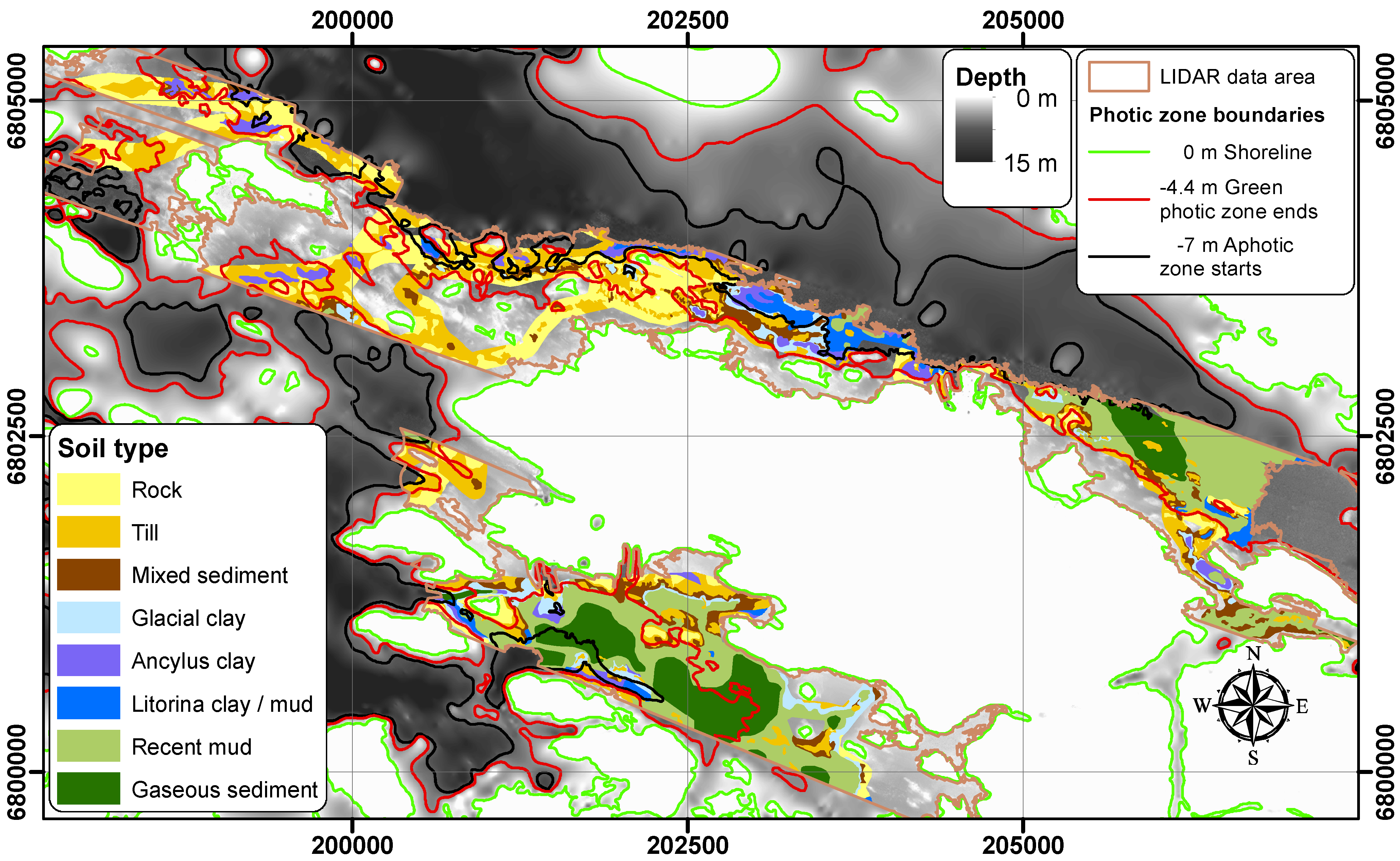
In this study, the clustering result of the bathymetric LiDAR waveform data is interpreted with respect to the sea bottom substrate type and photic zone delineation. The Geological Survey of Finland (GSF) performed acoustic sounding in the study area in 2000 and in 2008 to map the seabed geology [11,12]. The survey lines of these soundings are presented in Figure 1. Bottom sediment type was analyzed along the survey lines, and the information about the topmost layer of the sea bottom was extrapolated based on the side scanning sonar data to form a sediment map (see Figure 2).

Figure 1. Survey areas: the gray-scale and color-coded rasters represent seabed elevation interpolated from the sonar and bathymetric LiDAR measurements. The LiDAR survey areas are highlighted in color. The sonar survey lines are also indicated in the figure.

Figure 1. Survey areas: the gray-scale and color-coded rasters represent seabed elevation interpolated from the sonar and bathymetric LiDAR measurements. The LiDAR survey areas are highlighted in color. The sonar survey lines are also indicated in the figure.

The LiDAR return pulse waveform contains also information on benthic vegetation. The main features affecting the bottom return pulse waveform are the color, height and structure of the vegetation. The spatial distribution of the vegetation is dominated by the sediment type, as well as photic conditions. According to its optical properties, sea bottom flora in the study area can be roughly divided into green (such as Cladophora, for example) and brown/red (such as Polysiphonia fucoides, for example) vegetation [13]. It has been suggested in [13] that the photic zone for green vegetation extends down to −4.4 m, while for brown or red vegetation, the photic zone extends down to −7 m.

2.2. Data Acquisition and Survey Conditions

According to the survey report and aerial images taken during the overflight, the weather conditions were good, clouds were high and the sea was calm with no fog in the survey area. The survey was performed in September when the amount of algae in the water was decreasing. The Secchi readings ranged from 2.3 to 3 m, which, according to the data provider, means that data could be acquired from up to 5.7, …, 7.5-m deep waters. This is in good agreement with the result that the aphotic zone starts at about a 5, …, 8-m depth in the study area (see Figure 9 in [14]). Sea level was 20 cm above the reference value at the time of the data acquisition.

Figure 2. Reference map derived from the depth map and Geological Survey of Finland (GSF) survey data. The map is obtained by complementing the map of [12] (Appendix 3) with data along the survey lines in [11]. The map is recompiled by the authors using the ArcGIS software. The photic zones are also indicated on the map. (The data used in this figure was obtained from Posiva Oy with permission.)

Figure 2. Reference map derived from the depth map and Geological Survey of Finland (GSF) survey data. The map is obtained by complementing the map of [12] (Appendix 3) with data along the survey lines in [11]. The map is recompiled by the authors using the ArcGIS software. The photic zones are also indicated on the map. (The data used in this figure was obtained from Posiva Oy with permission.)

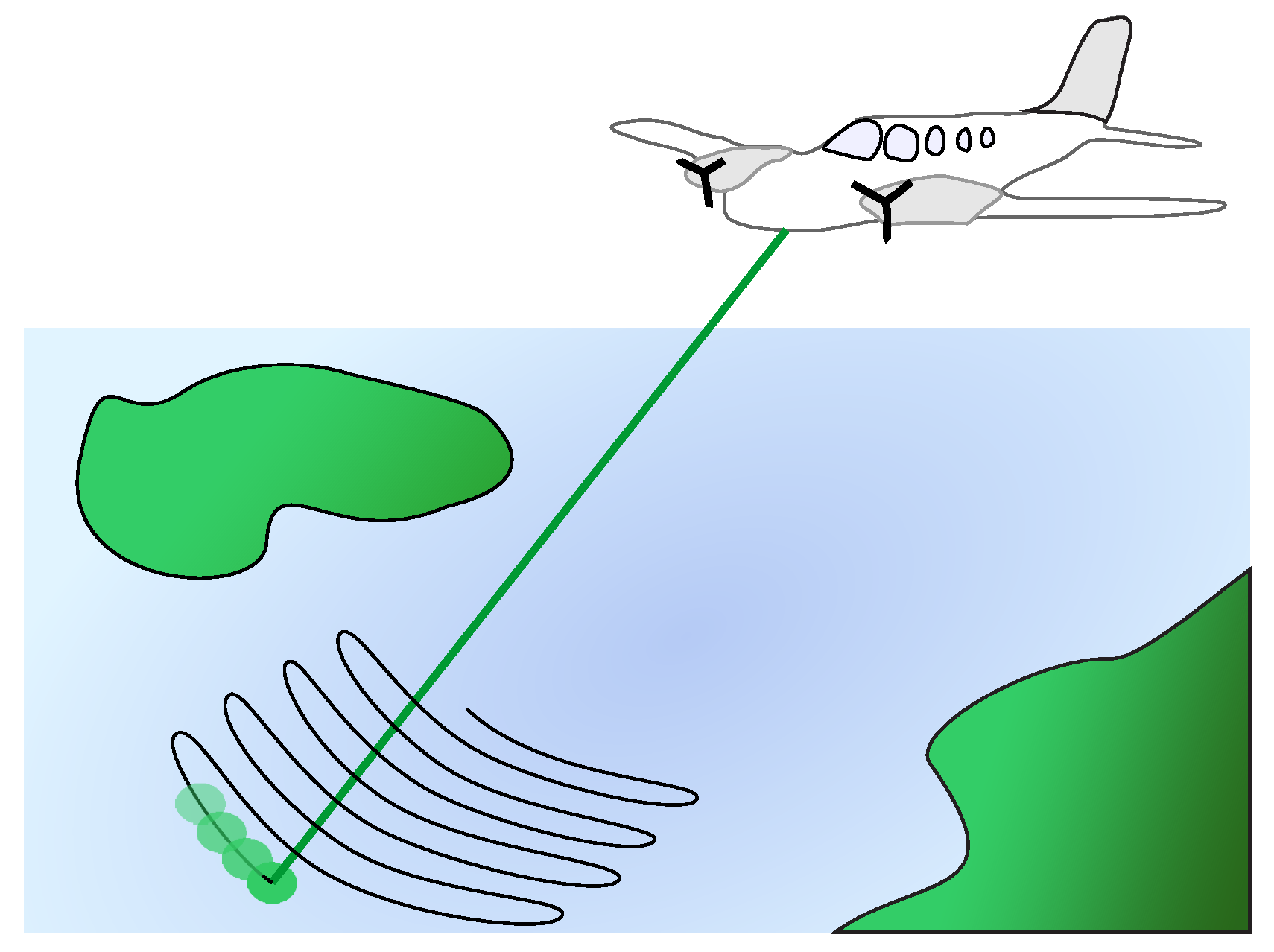
Survey data were acquired using the HawkEye II bathymetric LiDAR system [15]. The LiDAR system uses a green laser with a wavelength of 532 nm, optimized for the turbid coastal waters’ light attenuation characteristics. The system also uses an infrared laser at 1064 nm for water surface detection. The system contains a stabilized servo-controlled lens system that scans ground in a predefined pattern, as shown in Figure 3. The detector contains four sensors arranged in two rows. Each sensor records a waveform from the same emitted laser pulse at a 1-GHz sampling rate. In the HawkEye II LiDAR system, the received laser beam is divided into deep and shallow channels, with the former having a larger field of view (about 50 mrad) to enable signal acquisition from deeper areas and the latter having narrower field of view (about 25 mrad) to enable better spatial resolution. In our study, only the shallow channel waveforms were used. The acquisition system is described in more detail in the technical report by Tulldahl and Wikström [16].

The dataset underlying this study contains already preclassified seabed depth data in LAS 1.2 format and the return pulse waveform data in a proprietary binary data format. The depth of the seabed is usually calculated based on the delay between the bottom and surface return pulses; however, in some cases, when there is no detectable bottom return pulse, water depth can be assessed based on the time delay of the drop in the waveform backscatter level. For depth data generation, the data provider [15] uses the Coastal Survey Studio (CSS) post-processing software, performing also wave height corrections and position refinement. The data position accuracy of the Hawk Eye II system is at least ±0.25 m in the vertical and ±2.5 m in the horizontal direction. The content available to our study for each data record is presented in Table 1.

Figure 3. HawkEye II scanning pattern.

Figure 3. HawkEye II scanning pattern.

Table 1. Data content for each LiDAR pulse obtained from the Airborne Hydrography AB(AHAB) HawkEye II system. The data written in italics were used in this study.

No. of waveforms	Data	Comment
1	Raman channel waveform	Water surface detection
1	Infrared channel waveform	Water surface detection
4	Deep channel waveform	4-pixel detector
4	Shallow channel waveform	4-pixel detector
2	Amplifier gain waveform	Shallow and deep channel
-	Detector pixel id	From LAS file
-	Point class	From LAS file
-	Ground position	From LAS file
-	Plane position	From flight data

Table 1. Data content for each LiDAR pulse obtained from the Airborne Hydrography AB(AHAB) HawkEye II system. The data written in italics were used in this study.

No. of waveforms	Data	Comment
1	Raman channel waveform	Water surface detection
1	Infrared channel waveform	Water surface detection
4	Deep channel waveform	4-pixel detector
4	Shallow channel waveform	4-pixel detector
2	Amplifier gain waveform	Shallow and deep channel
-	Detector pixel id	From LAS file
-	Point class	From LAS file
-	Ground position	From LAS file
-	Plane position	From flight data

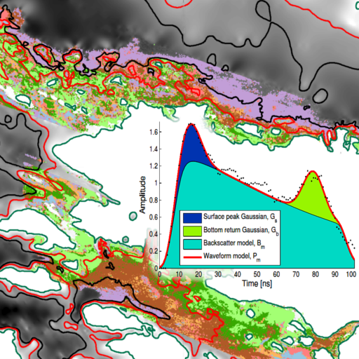
An example of the return pulse waveform of the bathymetric LiDAR is presented in Figure 4. The pulse can be separated into three components: the surface return pulse, the bottom return pulse and the water column backscatter. The mathematical functions used to model the waveform components are described in detail in Section 2.3. The waveform analysis and clustering algorithm contains the following steps:

• data preparation, waveform modeling and feature extraction
• feature/condition variable post-processing
• regression analysis to decrease the effect of the condition variables
• clustering.

The analysis procedure is illustrated in Figure 5 and described in more detail in the following sections.

Figure 4. (a) Bathymetric LiDAR waveform from the deep region. (b) Waveform modeling components.

Figure 4. (a) Bathymetric LiDAR waveform from the deep region. (b) Waveform modeling components.

Figure 5. Process flow of the algorithm for LiDAR waveform analysis.

Figure 5. Process flow of the algorithm for LiDAR waveform analysis.

2.3. Waveform Modeling and Feature Extraction

The waveforms were extracted from the proprietary binary file format using a tool provided by the AHAB company. The waveforms were combined with the original point data in the LAS 1.2 format using a common GPS timing key and stored in an LAS 1.4 file. For each LiDAR pulse, 12 waveforms were stored (see Table 1).

In data acquisition, a dynamic gain function is used in the receiver amplifier to emphasize deeper parts of the waveform. The gain waveform is included in the data for each set of four pixels (see Table 1). Before further pulse analysis, the amplitudes of the pixel waveforms were rescaled according to the gain waveforms.

The pulse waveforms were filtered using the Wiener filter for noise removal [17]. Wiener filtering is a well-established signal processing technique for removing a noise component from the signal given that the estimates of the noise and signal power spectra are available and assuming additive noise component [18]. The noise estimate was obtained by combining two segments of the pulse waveform, one from before the reflection from the water surface and the other from after the bottom reflection. Two samples of noise were used, as the properties of the noise component after the bottom return were clearly different from the solar and detector noise present in the waveform before the water surface return.

Separation of the backscatter, surface return and bottom return components of the waveform was accomplished using a constrained optimization algorithm to fit two Gaussian pulses $G_s$ and $G_b$, and a model of the backscatter $B_m$ to the pulse waveform P. The Gaussian pulses $G_s$ and $G_b$ model the water surface return and the sea bottom return, respectively. The optimization was done according to the criterion:

$$arg\underset{\theta }{min}∥P-P_m(\theta )∥,$$

(1)

where the waveform model $P_m(\theta )$ is expressed as:

$$\begin{array}{cc}\hfill P_m(\theta )=& G_s(h_1,t_1,w_1)\hfill \\ \hfill +& B_m(h_b,k,c_{sc},w_{sc},t_{start},t_{end},k_{end})\hfill \\ \hfill +& G_b(h_2,t_2,w_2)\hfill \end{array}$$

(2)

with the parameter vector:

$$\begin{array}{c}\hfill \theta =\{h_1,t_1,w_1,h_2,t_2,w_2,h_b,k,c_{sc},w_{sc},t_{start},t_{end},k_{end}\}.\end{array}$$

(3)

Here, h denotes amplitude, t denotes location in time, w is the width of the particular Gaussian pulse, k is the backscatter attenuation coefficient, $c_{sc}$ is the volume scattering loss and $w_{sc}$ is the width scale of the volume scattering loss of $B_m$. The subscripts 1 and 2 correspond to the Gaussian pulses $G_s$ and $G_b$, respectively, and start and end refer to the corresponding phases of the backscatter. The model used in the constrained optimization is designed from the perspective of simple optimization for information extraction purposes and not from the physical standpoint. The model is a modified version of the LiDAR simulator described in [19]. The ortho-MADS direct search algorithm implemented as a part of the NOMAD [20] software package was used [21]. The optimization method is sensitive to the initial parameters, such as the selection of the starting point, as well as lower and upper bounds for the parameters. Constraints were also applied to limit the locations of the pulses $G_s$, $G_b$ and $B_m$ with respect to one another. Usually a couple of optimization runs involving refinements of the limits and the starting point are needed to find an acceptable solution between P and $P_m$, especially at shallow regions.

In shallow waters, pulse modeling is totally relying on the constraints and boundaries, while at deeper regions, it is easier to separate surface and bottom return pulses from the backscatter. However, the backscatter does not always follow exponential attenuation, as turbidity conditions may vary as a function of depth; however, this is not modeled in this study. Smooth parametrization of the optimization constraints for each depth zone is critical, as otherwise, there will be transitions in the distributions of the extracted variables that are problematic to correct with statistical analysis.

The backscatter model is obtained as a result of the convolution operation between the LiDAR shot pulse $P_{shot}$ and the water column effect model:

$$B_m=\frac{h_b}{h_{norm}}·P_{shot}*\frac{H(t-t_{start})e^{-k(t-t_{start})}{e}^{-k_{end}(t-t_{end})H(t-t_{end})}}{1+c_{sc}{\left(w_{sc}(t-t_{start})\right)}^2}.$$

(4)

$h_{norm}$ scales the maximum of the convolution result into a unit scale for easier calculation of the optimization bounds. $H\left(t\right)$ denotes the unit step function. The LiDAR shot pulses were found to be quite close to Gaussian with the main difference in that the real pulses had trailing tails. In this study, a mean of 1000 unit scaled pulses was used as a model for the shot pulse. The parameters $c_{sc}$ and $w_{sc}$ were determined empirically and were constant during the optimization. The values $c_{sc}=1.0$ and $w_{sc}=0.0002$ were used. $k_{end}$ is a depth-dependent variable simulating the backscatter decaying off. The empirically-found relation $k_{end}=-0.12e^{-0.17z_{opt}}$ was used.

After the waveform parameters in θ are optimized, the bottom return pulse is estimated as $P_{bottom}=P-B_m-G_s$. Any noise spikes left after modeling were removed by cutting bottom return pulse tails at the distance where $G_b$ falls below 1% of the maximum.

Feature and Condition Variable Extraction

In this study, the term feature is used for the variables extracted from the bottom return pulse and condition for the variables describing the process of LiDAR pulse propagation and environmental conditions. In the subsequent analysis, our aim is to eliminate the effect of the conditions on the features and to preserve only the components describing the benthic cover of the seabed. The extracted conditions are presented and defined in Table 2, while the features are listed in Table 3. Most of the bottom return pulse features used in this study are similar to the ones described in Tulldahl et al. [5].

Table 2. List of condition variables.

Variable	Name	Source	Use
$z_{pp}$	Peak to peak time	$t_2-t_1$	Water column length
$W_p$	Water surface peak	$P\left(t_1\right)-B_m\left(t_1\right)$	Wave/surface condition
$B_p$	Backscatter peak	$P\left(t_1\right)-h_1$	Fast pulse to pulse changes
z	Depth	Survey data	Data checks
$z_{opt}$	In-water optical axis path	$zcos\alpha$	Bounds in optimization
α	Off-nadir in-water angle	Estimated from survey data	Depth → optical depth
β	Azimuth scan angle	Estimated from survey data	Pixel calibration
$A_g$	Gain estimate	Low-pass filtered $B_p$	Linearization
$S_h$	Cross-track seabed slope	Estimated from survey data	Slope compensation
$S_f$	Forward seabed slope	Estimated from survey data	Slope compensation
k	Water column attenuation	k	Water column attenuation
$F_{pix}$	Pixel number	Survey data	Pixel calibration
$R_{back}$	Backscatter residual	Maximum of median filtered residual	High vegetation

Table 2. List of condition variables.

Variable	Name	Source	Use
$z_{pp}$	Peak to peak time	$t_2-t_1$	Water column length
$W_p$	Water surface peak	$P\left(t_1\right)-B_m\left(t_1\right)$	Wave/surface condition
$B_p$	Backscatter peak	$P\left(t_1\right)-h_1$	Fast pulse to pulse changes
z	Depth	Survey data	Data checks
$z_{opt}$	In-water optical axis path	$zcos\alpha$	Bounds in optimization
α	Off-nadir in-water angle	Estimated from survey data	Depth → optical depth
β	Azimuth scan angle	Estimated from survey data	Pixel calibration
$A_g$	Gain estimate	Low-pass filtered $B_p$	Linearization
$S_h$	Cross-track seabed slope	Estimated from survey data	Slope compensation
$S_f$	Forward seabed slope	Estimated from survey data	Slope compensation
k	Water column attenuation	k	Water column attenuation
$F_{pix}$	Pixel number	Survey data	Pixel calibration
$R_{back}$	Backscatter residual	Maximum of median filtered residual	High vegetation

Table 3. List of extracted features from the bottom pulse.

Feature	Description of pulse feature
$A_{max}$	Maximum amplitude
$W_{25\%}$	Pulse width at 25 % level of maximum amplitude
$W_{50\%}$	Pulse width at 50 % level of maximum amplitude
$t_{rise25\%}$	Rise time from 25 % level to maximum amplitude
$t_{rise50\%}$	Rise time from 50 % level to maximum amplitude
$t_{fall25\%}$	Fall time from maximum amplitude to 25 % level
$t_{fall50\%}$	Fall time from maximum amplitude to 50 % level
$R_{back}$	Maximum of median filtered backscatter residual

Table 3. List of extracted features from the bottom pulse.

Feature	Description of pulse feature
$A_{max}$	Maximum amplitude
$W_{25\%}$	Pulse width at 25 % level of maximum amplitude
$W_{50\%}$	Pulse width at 50 % level of maximum amplitude
$t_{rise25\%}$	Rise time from 25 % level to maximum amplitude
$t_{rise50\%}$	Rise time from 50 % level to maximum amplitude
$t_{fall25\%}$	Fall time from maximum amplitude to 25 % level
$t_{fall50\%}$	Fall time from maximum amplitude to 50 % level
$R_{back}$	Maximum of median filtered backscatter residual

The stretching effect on the LiDAR bottom return pulse caused by the bottom slope has been studied in [9]. In our study, this effect was taken into account by defining two condition variables: the cross-track seabed slope $S_h$ and the forward seabed slope $S_f$. In addition to slope, these variables also consider the aspect information of the bottom surface, so that $S_f$ quantifies the angle of the bottom surface in the direction of the LiDAR pulse propagation vector $V_{pulse}$ and $S_h$ quantifies the angle of the bottom surface in the direction perpendicular to $V_{pulse}$. These variables were derived from the estimate of the bottom surface gradient, calculated using the method described in Kumpumäki and Lipping [22] and stored as a raster data file in 1-m spatial resolution.

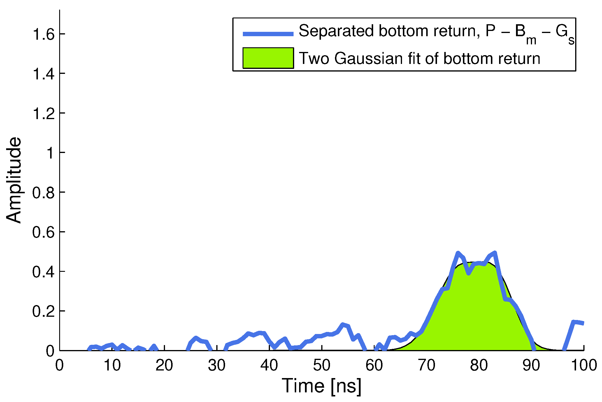
The bottom return pulse $P_{bottom}$, obtained as the result of the modeling procedure described above, has a low signal-to-noise ratio. In order to acquire a noise-suppressed continuous time version of the bottom return pulse for feature extraction, the bottom return pulse was further modeled using a combination of two Gaussian pulses ($G_{bottommodel}$). An example of fitting a double Gaussian model to a bottom return pulse is shown in Figure 6. The model $G_{bottommodel}$ was constrained by the following rules: amplitude parameter was 1.1-times the maximum; all parameters were positive; and width and location parameters were constrained by the bottom return pulse analysis window where the bottom return pulse was centered.

Figure 6. Modeling of the bottom return pulse extracted from the waveform shown in Figure 4a.

Figure 6. Modeling of the bottom return pulse extracted from the waveform shown in Figure 4a.

Backscatter residual $R_{back}$ is also included as a feature variable, as the spatial variability of this feature suggests that it may contain information about tall benthic vegetation. $R_{back}$ is calculated as the maximum deviation from the median filtered version of the signal $P-B_m-G_s-G_{bottommodel}$ between the peak locations $t_1$ and $t_2$.

2.4. Feature and Condition Variable Post-Processing

The features and condition variables contain outliers after the pulse optimization and feature extraction phases. Outlier removal was accomplished by projecting the features to the depth-feature plane and removing the outliers by analyzing each feature in one meter depth slices. Erroneous features and outliers were removed using a rule-based decision logic.

During the data acquisition, the overall gain of the signal amplifier was adjusted to keep the signal level as high as possible. The gain variation $A_g$ was estimated based on the surface return peak ($W_p$) and backscatter peak ($B_p$) variables. These variables are uncorrelated with the bottom surface properties, and the slow component of the dynamics of these variables can be used to estimate the changes in the amplifier gain. The time series of the variables were low-pass filtered by averaging time series generated using bootstrapped interpolations. This method is insensitive to outliers, enables one to fill gaps and produces a continuous time representation of the time series. The time series of the four sensor pixels were processed separately, and the signals were averaged to obtain the overall gain estimate.

Azimuth scan angle and pixel-dependent correction was also applied. For each scan line, a correction value was calculated for each point by finding the dependency between the pixel number $F_{pix}$, azimuth scan angle β and gain calibrated version of the backscatter peak $B_p$.

2.5. Regression Modeling

Regression modeling was used to compensate for the effect of the conditions on the bottom return properties. In the following, we will denote the number of data points used for the regression modeling procedure by N (in our case $N=2,219,607$), the number of feature variables by L and the number of condition variables by $K_l$. For each feature variable, a linear regression:

$${\mathbf{y}}_l={\mathbf{X}}_l{\mathbf{b}}_l+{\widehat{\mathbf{y}}}_l,l=1,\dots ,L$$

(5)

was estimated. Here, ${\mathbf{y}}_l$ are $N\times 1$ vectors of feature variables calculated from the N data waveforms, ${\mathbf{b}}_l$ are $K_l\times 1$ vectors of regression coefficients, ${\widehat{\mathbf{y}}}_l$ are $N\times 1$ vectors of the "cleaned" feature variables (i.e., feature variables with the effect of the condition variables removed) and ${\mathbf{X}}_l$ are $N\times K_l$ design matrices constructed for each feature variable and initiated by selectively inserting conditions from Table 2. Before calculating the regression coefficients, the design matrices were modified using a stepwise fitting procedure to remove irrelevant variables. As for different features different sets of condition variables were relevant, the size of the design matrix differs for different feature variables.

The regression coefficient vectors ${\mathbf{b}}_l$ were estimated by:

$${\mathbf{b}}_l={\left({\mathbf{X}}_l^T{\mathbf{X}}_l\right)}^{-1}{\mathbf{X}}_l^T{\mathbf{y}}_l,l=1,\dots ,L.$$

(6)

Finally, the condition variable-compensated feature variables for individual data points were obtained from:

$${\widehat{\mathbf{y}}}_l={\mathbf{y}}_l-{\mathbf{X}}_l{\mathbf{b}}_l,l=1,\dots ,L.$$

(7)

After the regression model corrections, features in the matrix $\widehat{\mathbf{Y}}=[{\widehat{\mathbf{y}}}_1,\dots ,{\widehat{\mathbf{y}}}_L]$ were checked against the depth variable to verify that no systematic depth dependencies remained.

2.6. Feature Clustering

Clustering of features contained in the matrix $\widehat{\mathbf{Y}}$ was performed in two steps. First the self-organizing map (SOM) [23] was used to map the feature vectors onto a lattice of cells [24]. SOM is an artificial neural network used for unsupervised learning. The SOM learning algorithm maps the data represented by a set of features onto a cell lattice so that the cells representing similar feature vectors appear close to each other in the lattice. The learning procedure is unsupervised; rather than training the algorithm based on some ground truth learning dataset, intrinsic similarities in the pulse waveforms are detected. The number of cells in the lattice is usually much higher than the number of final clusters.

The mapping procedure was performed using the MATLAB SOM Toolbox [25]. The SOM was constructed as a hexagonal toroid lattice of size $50\times 50$, leading to 2500 cells. On average, around 890 data points were mapped to each SOM cell. The reason for using such a large number of cells was that the different benthic cover types are not evenly represented in the data and smaller lattice would have missed some important classes.

In the second step, the cells in the SOM lattice were grouped into a smaller number of final clusters, and all LiDAR data points were assigned to the best matching cluster. This step was performed using the SOM neighborhood distance matrix method described in [26]. The number of clusters is determined by the method based on the structure of the obtained cell lattice. By changing the level at which the grouping algorithm is terminated, different numbers of final clusters can be obtained. The SOM lattice structure and the cell grouping result for various levels of grouping are presented in the supplement.

3. Results

In Figure 7, the distributions of the bottom return pulse waveforms mapped to the seven clusters obtained when terminating the SOM cell grouping at Level 5 are presented. All of the results for Levels 1 to 5 are available in the supplement. The distribution of the $R_{back}$ feature variable is given separately in Figure 8, as this variable describes the backscatter and not the pulse waveforms. The clusters clearly differ from one another with respect to the feature variables listed in Table 3. There are also significant differences in the value of the $R_{back}$ variable among the clusters.

To evaluate the meaningfulness of the clustering result, the correspondence between the clusters and the bottom substrate type was assessed for the LiDAR data points along the sonar survey lines (see Figure 1 for the survey lines). Table 4 shows the positive predictive value of the clusters with respect to the vegetation zones and substrate types. Here, the rock, till and mixed substrate classes are grouped as hard bottom and the clay, mud and gaseous substrate classes as soft bottom. From these results, the correspondence between the clusters and the reference data can be observed. Cluster 1, for example, indicates a soft bottom in deeper sea areas without a significant amount of vegetation (as is most frequent in the aphotic zone), while Cluster 3 is indicative of green vegetation in shallow areas. In Cluster 6, the value of the $R_{back}$ feature variable is significantly higher compared to the other clusters, indicating high vegetation in shallow areas with mostly soft bottom.

Figure 7. Bottom return pulse shapes and their distributions for the seven clusters.

Figure 7. Bottom return pulse shapes and their distributions for the seven clusters.

Figure 8. Boxplot representation of the distribution of the $R_{back}$ feature variable in the seven clusters.

Figure 8. Boxplot representation of the distribution of the $R_{back}$ feature variable in the seven clusters.

The depth of the sea bottom is determined from the delay between the surface return and the bottom return and can be used as additional information when interpreting the clustering results. In Table 5, the positive predictive value of the clusters with respect to the substrate type is shown separately for the three depth zones. Indeed, similar return pulse waveforms may correspond to different bottom classes in different environments. For example, Cluster 1, with a relatively sharp waveform (see Figure 7), indicates a high probability of mud or clay in the deeper aphotic zone, while a similar return pulse obtained in the shallow green vegetation regions indicates a hard substrate.

Table 4. Positive predictive value (PPV) of the obtained clusters with respect to the substrate type (hard/soft) and vegetation zone.

		1	2	3	4	5	6	7
Shallow areas (0…4.4 m)	Hard	6,40	49,19	35,71	26,64	32,44	22,15	9,38
green photic zone	Soft	0,28	15,23	54,00	14,95	35,31	40,89	11,05
Mid depth (4.4…7 m)	Hard	9,20	9,30	1,82	28,41	13,23	10,99	15,59
red photic zone	Soft	35,19	23,14	4,36	24,58	15,90	23,03	49,10
Deep areas (> 7 m)	Hard	6,63	0,00	0,48	1,96	0,39	0,94	1,81
aphotic zone	Soft	42,30	3,14	3,63	3,46	2,72	2,00	13,07
$N_{clust}$		3967	860	826	1070	2056	1702	3656

Table 4. Positive predictive value (PPV) of the obtained clusters with respect to the substrate type (hard/soft) and vegetation zone.

		1	2	3	4	5	6	7
Shallow areas (0…4.4 m)	Hard	6,40	49,19	35,71	26,64	32,44	22,15	9,38
green photic zone	Soft	0,28	15,23	54,00	14,95	35,31	40,89	11,05
Mid depth (4.4…7 m)	Hard	9,20	9,30	1,82	28,41	13,23	10,99	15,59
red photic zone	Soft	35,19	23,14	4,36	24,58	15,90	23,03	49,10
Deep areas (> 7 m)	Hard	6,63	0,00	0,48	1,96	0,39	0,94	1,81
aphotic zone	Soft	42,30	3,14	3,63	3,46	2,72	2,00	13,07
$N_{clust}$		3967	860	826	1070	2056	1702	3656

Table 5. Positive predictive value (PPV) of the obtained clusters with respect to the substrate class and vegetation zone. Here, PPV is calculated separately for the three vegetation zones.

		1	2	3	4	5	6	7
	Rock	47,92	18,23	16,46	32,81	8,26	2,61	10,71
	Till	47,17	47,65	18,08	25,39	25,41	20,88	31,73
Shallow areas (0, …, 4.4 m)	Mixed sediment	0,75	10,47	5,26	5,84	14,21	11,65	3,48
green photic zone	Clay	0,75	12,45	11,47	9,21	3,52	19,57	2,28
	Mud	1,13	10,65	41,16	19,78	37,26	30,85	36,28
	Gaseous sediment	2,26	0,54	7,56	6,97	11,34	14,45	15,53
$N_{clust}$		265	554	741	445	1393	1073	747
	Rock	0,80	0,72	1,96	11,82	6,68	1,90	1,82
	Till	7,61	7,89	13,73	26,63	27,38	13,47	10,44
Mid depth (4.4, …, 7 m)	Mixed sediment	12,32	20,07	13,73	15,17	11,35	16,93	11,84
red photic zone	Clay	10,73	12,90	0,00	7,23	6,51	9,15	14,76
	Mud	54,17	4,30	49,02	16,93	41,90	50,09	37,76
	Gaseous sediment	14,37	54,12	21,57	22,22	6,18	8,46	23,38
$N_{clust}$		1761	279	51	567	599	579	2365
	Rock	0,15	0,00	0,00	1,72	0,00	0,00	0,55
	Till	6,29	0,00	8,82	31,03	10,94	0,00	10,11
Deep areas (> 7 m)	Mixed sediment	7,11	0,00	2,94	3,45	1,56	32,00	1,47
aphotic zone	Clay	27,67	14,81	8,82	12,07	15,63	10,00	12,87
	Mud	48,53	29,63	58,82	48,28	50,00	56,00	39,89
	Gaseous sediment	10,25	55,56	20,59	3,45	21,88	2,00	35,11
$N_{clust}$		1941	27	34	58	64	50	544

Table 5. Positive predictive value (PPV) of the obtained clusters with respect to the substrate class and vegetation zone. Here, PPV is calculated separately for the three vegetation zones.

		1	2	3	4	5	6	7
	Rock	47,92	18,23	16,46	32,81	8,26	2,61	10,71
	Till	47,17	47,65	18,08	25,39	25,41	20,88	31,73
Shallow areas (0, …, 4.4 m)	Mixed sediment	0,75	10,47	5,26	5,84	14,21	11,65	3,48
green photic zone	Clay	0,75	12,45	11,47	9,21	3,52	19,57	2,28
	Mud	1,13	10,65	41,16	19,78	37,26	30,85	36,28
	Gaseous sediment	2,26	0,54	7,56	6,97	11,34	14,45	15,53
$N_{clust}$		265	554	741	445	1393	1073	747
	Rock	0,80	0,72	1,96	11,82	6,68	1,90	1,82
	Till	7,61	7,89	13,73	26,63	27,38	13,47	10,44
Mid depth (4.4, …, 7 m)	Mixed sediment	12,32	20,07	13,73	15,17	11,35	16,93	11,84
red photic zone	Clay	10,73	12,90	0,00	7,23	6,51	9,15	14,76
	Mud	54,17	4,30	49,02	16,93	41,90	50,09	37,76
	Gaseous sediment	14,37	54,12	21,57	22,22	6,18	8,46	23,38
$N_{clust}$		1761	279	51	567	599	579	2365
	Rock	0,15	0,00	0,00	1,72	0,00	0,00	0,55
	Till	6,29	0,00	8,82	31,03	10,94	0,00	10,11
Deep areas (> 7 m)	Mixed sediment	7,11	0,00	2,94	3,45	1,56	32,00	1,47
aphotic zone	Clay	27,67	14,81	8,82	12,07	15,63	10,00	12,87
	Mud	48,53	29,63	58,82	48,28	50,00	56,00	39,89
	Gaseous sediment	10,25	55,56	20,59	3,45	21,88	2,00	35,11
$N_{clust}$		1941	27	34	58	64	50	544

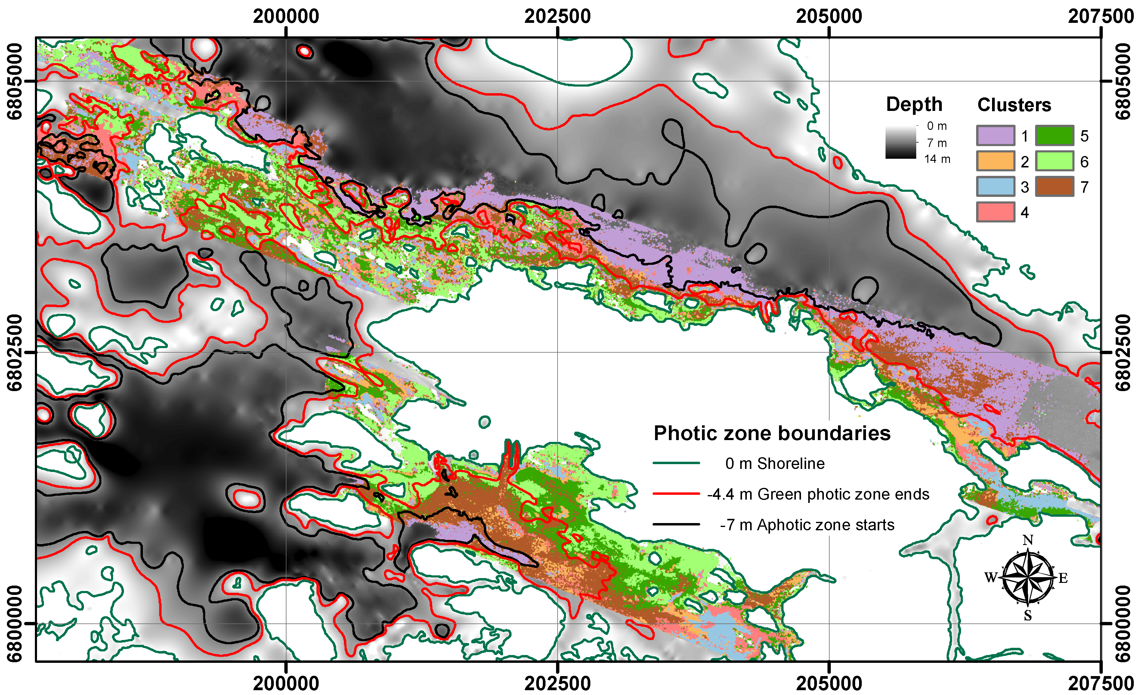
We also projected back the cluster-labeled data points to form a cluster map of the study area (Figure 9). The map was created as a $4\times 4$-m raster where the cluster of each pixel was determined as the mode of the cluster values of the data points inside a circle of 8-m radius around the center of the pixel. For visual clarity, a 3 × 3 cross-shaped mode filter was applied to the raster. By following the photic zone borders, it can be seen that they coincide relatively well with cluster boundaries, indicating a change in bottom return pulse properties.

Figure 9. Cluster map of the study area with seven clusters. The photic zones are also indicated on the map.

Figure 9. Cluster map of the study area with seven clusters. The photic zones are also indicated on the map.

4. Discussion

In this section, some issues related to the proposed methodology are considered first, after which the results of bottom return pulse clustering are discussed.

Figure 10. Shallow water (a) and deep water (b) bottom return pulse decomposition.

Figure 10. Shallow water (a) and deep water (b) bottom return pulse decomposition.

In the course of algorithm development, it was found that in shallow waters the constraints of the pulse fitting procedure became crucial (see Section 2.3). In Figure 10, two return pulses are shown, one from a location where the in-water optical axis path length is 1.8 m (Figure 10a) and the other from a location where the in-water optical axis path length is 7.5 m (Figure 10b). In the case of shallow waters, the three waveform components are highly overlapping. Separation of the components would not be possible without additional information contained in the optimization constraints. The minimum depth from which the presented modeling method is able to reliably extract data is about 1 m. However, in shallow areas, the probability of modeling errors starts to increase. Modeling errors were dealt with by the outlier removal step of the algorithm (see Section 2.4). Separation of the model components of a waveform originating from deeper waters is easier, as the backscatter decay can now be directly estimated without relying on constraints (Figure 10b). It is also worth noting that the surface return varies spatially depending on the wave conditions. This can be seen by comparing the shapes of the surface return components of the two pulses presented in Figure 10.

Figure 11. Partial regression plots of feature $A_{max}$ against condition variables selected by the stepwise fitting procedure. The variables are in the normalized scales.

Figure 11. Partial regression plots of feature $A_{max}$ against condition variables selected by the stepwise fitting procedure. The variables are in the normalized scales.

An example of the results of regression modeling described in Section 2.5 for the feature variable $A_{max}$ is illustrated in Figure 11. After the stepwise fitting procedure, nine condition variables remained in the corresponding design matrix. The effect of individual condition variables on the $A_{max}$ feature can be seen in the panels of the figure. Note that the cross-track slope of the seabed is assessed as deviation from the flat surface, and therefore, the distribution is one-sided. The distribution of the estimated water column attenuation has a long and narrow tail, indicating that the data contain some points from significantly more turbid water than most of the data. Only first order models were used in this study, as reliable fitting of the higher order terms was not plausible due to the uneven distribution of features with respect to variations in depth. The use of a higher order model could yield better correction for the particular condition variable, but is more sensitive to fitting errors and requires a significant amount of data from the whole range of the corresponding variables.

It can be seen from Figure 11 that while some of the nine condition variables, such as peak-to-peak time and gain estimate, for example, have strong influence on $A_{max}$, the impact of other variables, such as water surface peak, for example, is quite small. In addition to correcting for the conditions, plotting the regression lines, as shown in Figure 11, is useful when assessing the influence of various environmental and data acquisition related parameters on the features extracted from the bottom return pulse.

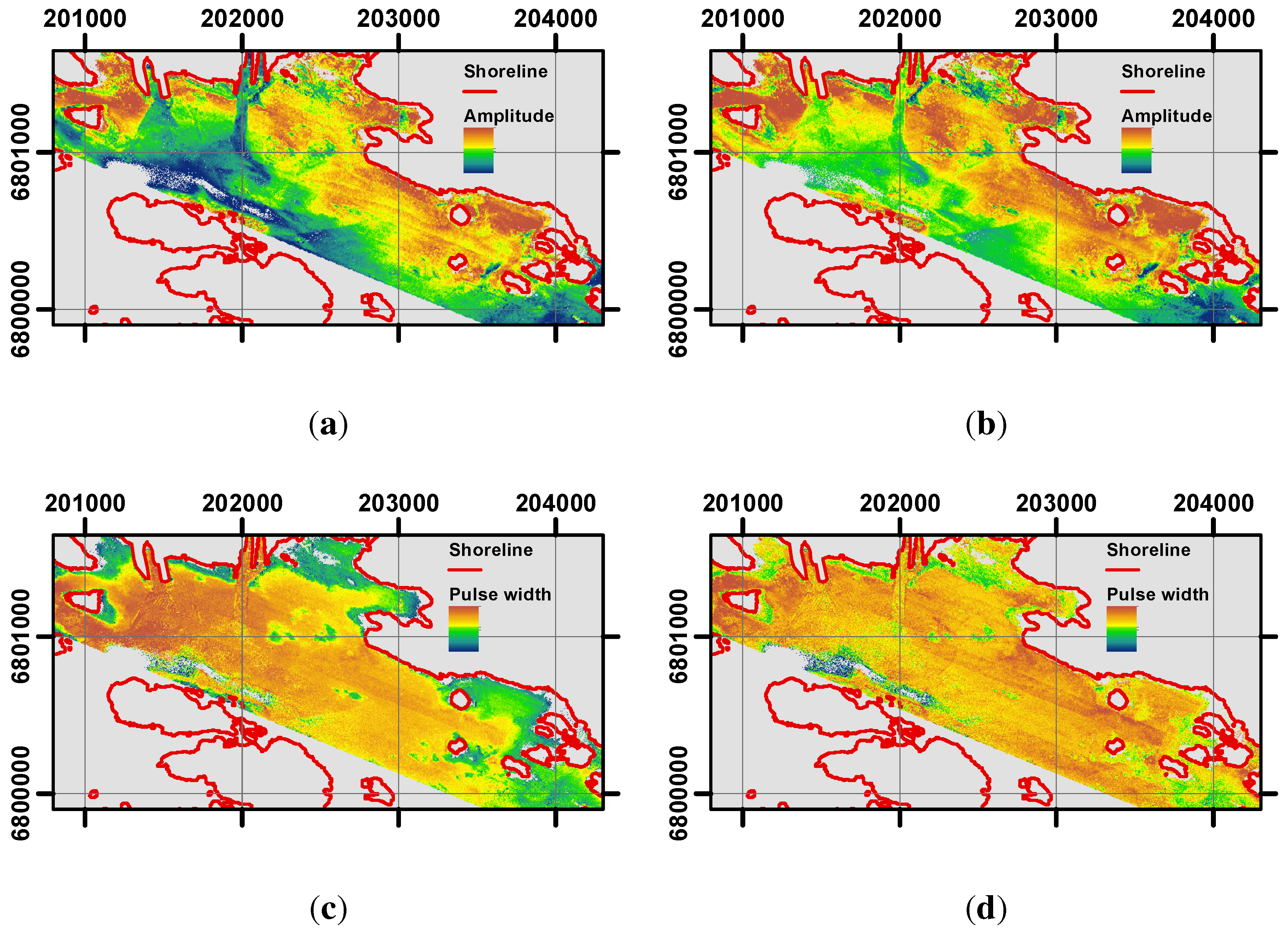
In Figure 12a,b, uncorrected and corrected versions of the amplitude feature are presented. The most significant difference in the figures is that the amplitude feature value is increased in deep areas to compensate for higher attenuation, and the feature values elsewhere are scaled accordingly. Other corrections are mostly local to some conditions present at a particular location (e.g., waves or some system dependent conditions). In the northern part of the study area (not shown in the figure), large discrepancies in amplitudes and other feature variables between the flight lines were observed. After the corrections, these discrepancies were suppressed. Without the regression model corrections, these errors were large enough to cause the formation of new clusters in the clustering phase.

Figure 12. Effects of the feature correction. Note that scales are not directly comparable after the corrections. (a): Uncorrected amplitude; (b): Corrected amplitude; (c): Uncorrected pulse width; (d): Corrected pulse width.

Figure 12. Effects of the feature correction. Note that scales are not directly comparable after the corrections. (a): Uncorrected amplitude; (b): Corrected amplitude; (c): Uncorrected pulse width; (d): Corrected pulse width.

When interpreting the results presented in Table 4 and Table 5, it should be kept in mind that the proposed clustering method is purely descriptive and does not use any ground truth data for training the classifier. The reference data give only rough indication of the benthic environment, and as described in [13], the study area is challenging from the point of view of benthic cover type mapping with highly varying substrate type and diverse marine vegetation. Therefore, the results evaluating the correspondence between the clusters and the reference data indicate the feasibility of the proposed methodology for describing the benthic environment, as represented by the bathymetric LiDAR bottom return pulse waveform, rather than provides a mapping of the benthic cover type to predeïňĄned classes. The methodology is useful for mapping large coastal areas to detect the structure and variation in the benthic environment. However, even if interpreted as a classification attempt, the results are comparable to those presented, for example, in [2].

Here, we used seven clusters to describe the bathymetric LiDAR bottom return pulse waveform. It is clear that the actual amount of benthic cover types in the study area is much higher. When terminating the SOM cell grouping algorithm at a lower level, more clusters are obtained. The results for 7, 12, 17, 21 and 52 clusters (corresponding to Levels 5 to 1, respectively) are presented in the supplement. The cluster maps for different grouping levels were found to be consistent: new clusters at lower levels appeared within the larger clusters of higher levels, while the borders of the larger clusters remained approximately in place.

A comparison of the clustering result with the substrate classes is further hindered by the fact that the sonar data were acquired mainly in 2008, while the bathymetric LiDAR data were acquired four years later. Mykkänen et al. [27] have studied the resuspension and the flow of sediment particles in the Eurajoensalmi Bay and found that in calm weather, the sediments carried by the Eurajoki River flow in the water surface layer towards the open seas, while at the sea bottom, the direction of flow is the opposite. In case of stormy weather, however, the surface water is pushed towards the coast, while in the bottom layers, water flows towards the open seas. This flow may change the distribution of sediments somewhat in the course of time. It is clear, however, that changes in the sediment distribution between the sonar and LiDAR data acquisition instances would pose additional difficulties to our evaluation and that the results would be even better if no changes would have occurred.

5. Conclusions

The aim of this study was to present a methodological framework for clustering the bathymetric LiDAR bottom return pulses according to the shape of their waveform. In contrast to most studies concentrating on the application of bathymetric LiDAR to detect certain environmental features, the presented clustering method is unsupervised and purely descriptive, not using any ground truth data in training the classifier. A comparison with what is known about the substrate types based on sonar data [12] and the photic zone delineation in the region as indicated in [10] shows that the obtained clusters are indeed meaningful and have descriptive value.

Classification of bathymetric LiDAR features based on detailed ground truth data is valuable, but often limited to the particular study area. Instead of performing the field work concurrently with the bathymetric data acquisition, the proposed methodology is most useful in clustering and mapping the data acquired from large areas to discover the structure in habitat distribution and to focus the field work on the potentially most interesting regions. The clusters, their number, as well as their corresponding waveform shapes and ground truth classes would differ in different benthic environments and can be determined and refined by subsequent field studies.