A Method to Analyze the Potential of Optical Remote Sensing for Benthic Habitat Mapping

Abstract

Quantifying the number and type of benthic classes that are able to be spectrally identified in shallow water remote sensing is important in understanding its potential for habitat mapping. Factors that impact the effectiveness of shallow water habitat mapping include water column turbidity, depth, sensor and environmental noise, spectral resolution of the sensor and spectral variability of the benthic classes. In this paper, we present a simple hierarchical clustering method coupled with a shallow water forward model to generate water-column specific spectral libraries. This technique requires no prior decision on the number of classes to output: the resultant classes are optically separable above the spectral noise introduced by the sensor, image based radiometric corrections, the benthos’ natural spectral variability and the attenuating properties of a variable water column at depth. The modeling reveals the effect reducing the spectral resolution has on the number and type of classes that are optically distinct. We illustrate the potential of this clustering algorithm in an analysis of the conditions, including clustering accuracy, sensor spectral resolution and water column optical properties and depth that enabled the spectral distinction of the seagrass Amphibolis antartica from benthic algae.

1. Introduction

A fundamental issue with benthic classification of remotely imaged shallow water environments is determining the appropriate definition and number of benthic classes that: (i) optimizes the classification accuracy and precision [1]; and (ii) standardizes classification maps for ease of inter-comparisons [2]. The selection of classes and their descriptive resolution, i.e., biological detail [3], for a spectral library or training dataset, along with the image classification method, have typically been scene and sensor specific [4]. For multispectral imagery, the optimum spectral library could consist of image-derived or in situ spectra of pure endmembers (a discrete taxanomic unit i.e., high descriptive resolution) if the benthos in the scene is either homogeneous or was imaged with very high spatial resolution [5,6,7]. For a scene with patchy or heterogeneous benthos or that was imaged with moderate to low spatial resolution, the spectral library could contain classes pertaining to merged endmembers (i.e., mixed benthic assemblages) and low descriptive resolution [3,8,9]. Due to the spectral characteristics of the sensors used (e.g., SPOT, Landsat 5–7, IKONOS; QuickBird), the above studies mostly utilized supervised classification schemes with or without water column correction to produce benthic habitat maps (additional examples include [10,11,12]).

Hyperspectral sensors, in contrast, have enough spectral resolution and bands to potentially facilitate the spectral unmixing of an image spectrum based on the fractional cover of a subset of pure endmembers [13]. This has often led to the implementation of a spectral library of pure endmembers which would be linearly mixed either to pre-defined proportions such as in look-up table methods [14,15] or during spectral optimization in shallow-water inversion methods [16,17,18]. These methods have consequently achieved moderate to high benthic classification accuracies [14,19,20,21].

Previous studies with multispectral imagery have shown an inverse relationship between the number of benthic classes and the classification accuracy [1,3,8]. This same relationship has also been shown for hyperspectral imagery, see [21,22]. This raises the question of how to optimize the class selection, or equivalently how to merge classes of higher descriptive resolution in order to achieve both accurate and useful maps. Karpouzli et al. [23] observed that agglomerating pure endmembers based on their genera to obtain average spectra of coral, seagrass, macroalgae and sand, reduced the classification accuracy. Specifically high classification accuracy was obtained with more classes at finer descriptive resolution. This was attributed to the fact that the intra-class variability exceeded the inter-class separability—as it has been noted that some species of corals are spectrally similar to macroalgae and vice versa [24]. Clearly, averaging pure endmembers based on their genera, which seems a logical and ecologically meaningful step, may not maximize spectral separability between classes, and potentially leads to a higher probability of confusion during classification.

Furthermore increasing the descriptive resolution of the benthic classes may lead to a decrease in the precision of the resultant classification, particularly if sensor and environmental noise is taken into account. Such noise is a component of remotely sensed imagery originating from the sensor and from atmospheric, sunglint and air–water interface corrections that maybe imperfect at times [25,26]. The combined impact of sensor and environmental noise and spectral variability of a given taxonomic species observed in local and regional scales [27,28] act to degrade the inter-class spectral separability as described in Hedley et al. [26].

Minimizing confusion or uncertainty arising from spectrally similar classes necessitates a procedure to re-define the spectral library of endmembers into more distinct classes. Clustering is an approach that can merge those spectrally similar classes thereby reducing the spectral confusion in a spectral library. A variety of indices can be used to define the spectral similarity between two classes including root mean square error, spectral angle mapper [29] or spectral information divergence [30]. Though clustering is a common procedure in unsupervised classification [31,32,33,34], it is seldom performed on the endmember spectra that constitute the spectral library (for exceptions see [35,36,37]). Particularly on benthic spectra that are further modulated by the physical processes occurring in an optically variable water column. In this study we present a hierarchical clustering algorithm, based on linear discriminant coordinates, tailored for shallow-water inversion models that uses the intra-class variability to merge those classes in the benthic spectral library that overlap, i.e., are optically indistinguishable. Here, the intra-class variability incorporates the individual benthos’ natural spectral variability plus image-based sensor and environmental noise. The hierarchical clustering ceases when there is no spectral overlap in the variance between groups; and thus outputs a set of classes that are spectrally distinguishable under actual operational conditions. In combination with a shallow water forward model this hierarchical procedure was used to develop depth and water-column specific spectral libraries. The endmembers of which are spectrally distinguishable above the attenuating properties of an optically variable water column at depth. In addition we investigate the effect spectral resolution has on benthic class separability by analyzing the clustering from simulations using the following three sensors: Hyperspectral Imager for the Coastal Ocean (HICO); HyVista’s HyMap, and; Worldview-2 (WV2)—see Table 1 for a list of symbols and acronyms used in the text. Such information on the number and type (i.e., definition) of distinguishable classes at any given depth and water column optical properties helps to understand the potential of benthic classification from shallow water remote sensing imagery.

Table 1. List of symbols and acronyms used through the text.

Acronym	Definition
BA	Brown Algae
CSE	Spectral covariance matrix pertaining to NEΔrrs
GA	Green algae
HDC	Hierarchical clustering using linear Discriminant Coordinates
HICO	Hyperspectral Imager for the Coastal Ocean
LDA	Linear Discriminant Analysis
NEΔrrs	Sensor-environmental noise equivalent perturbation of rrs
RMSE	Root mean square error
RA	Red algae
SA	Semianalytical shallow water forward model
SD	Sediment
SG	Seagrass
SRF	Spectral response function
WV2	WorldView-2
ZSD	Secchi Depth (m)
G	Absorption coefficient of colored dissolved and detrital matter at 440 nm
H	Geometric depth of the water column
κ	Attenuation coefficient
k	Number of benthic classes
n	Number of wavebands
ρb	Benthic irradiance reflectance
P	Absorption coefficient of phytoplankton at 440 nm
rrs	Subsurface remote sensing reflectance
s	Number of LD eigenvectors
τm	Proportion of misclassified Linear Discriminant Functions between a pair of classes
X	Backscattering coefficient of suspended particles at 550 nm

Table 1. List of symbols and acronyms used through the text.

Acronym	Definition
BA	Brown Algae
CSE	Spectral covariance matrix pertaining to NEΔrrs
GA	Green algae
HDC	Hierarchical clustering using linear Discriminant Coordinates
HICO	Hyperspectral Imager for the Coastal Ocean
LDA	Linear Discriminant Analysis
NEΔrrs	Sensor-environmental noise equivalent perturbation of rrs
RMSE	Root mean square error
RA	Red algae
SA	Semianalytical shallow water forward model
SD	Sediment
SG	Seagrass
SRF	Spectral response function
WV2	WorldView-2
ZSD	Secchi Depth (m)
G	Absorption coefficient of colored dissolved and detrital matter at 440 nm
H	Geometric depth of the water column
κ	Attenuation coefficient
k	Number of benthic classes
n	Number of wavebands
ρb	Benthic irradiance reflectance
P	Absorption coefficient of phytoplankton at 440 nm
rrs	Subsurface remote sensing reflectance
s	Number of LD eigenvectors
τm	Proportion of misclassified Linear Discriminant Functions between a pair of classes
X	Backscattering coefficient of suspended particles at 550 nm

2. Methods

The overall goal is the development of a procedure that can quantitate the number and type of classes that are spectrally distinct for any given water column optical properties and depth from a spectral library of representative benthic species. We begin in Section 2.1 with a description of the benthic irradiance reflectance, ρ_b, library collected from the field and we then describe the hierarchical clustering algorithm in Section 2.2. Using the measured ρ_b data, the clustering algorithm outputs a library of endmembers that are spectrally separable above the total system’s variability but only suitable just below the air–water interface as the attenuating effects of a water column were not modeled. Given an estimated or known range of depths and water column optical properties in a scene, a semi-analytical shallow water forward model coupled with the clustering algorithm can be used to predict the benthic classes that are optically distinct. This procedure is detailed in Section 2.2.3.

2.1. Benthic Reflectance Library

A spectral library of pure endmembers was derived from in-air irradiance reflectance measurements of 22 benthic species collected from the Point Peron (32.2715°S, 115.6865°E) study site, Western Australia, on 22 August 2014 (Table 2). Benthic samples were collected with enough material to cover the 25° field of view of the ASD field spectrometer (1 nm resolution, 350–2500 nm coverage). However, the quantities of Posidonia sp. and Metagoniolithon stelliferum were too small to cover the field of view and these were placed over a substrate (sediment and rock/rubble respectively) that would normally be underneath. These samples were stored overnight in a tank that had aerated, flowing filtered seawater to minimize the effect of pigment degradation. The collected samples were then spectrally analyzed the following day on a bench top set up outside on a flat roof. All samples were placed on top of a large flat, non-reflective black tray. The ASD fiber optic was held using a retort stand at a constant 30 cm above the sample and at a small angle off nadir (approx. 10°) and a white reference plate was used to compute the reflectance for each spectral measurement at the same angular geometry. Furthermore, each benthic sample was stirred and mixed every three spectral measurements to capture the sub local-scale taxanomic spectral variability. With this setup approximately 30–40 in-air reflectance measurements were recorded for each (wet) benthos collected. At the time of sample collection (winter) the leaves of Posidonia sp. were in the dormant phases, and new leaves were not visible in the collection area. The leaves that were collected, however, were already detached and slightly senescent.

Table 2. List of the benthic species collected from the Point Peron study site.

Genera	Species
Brown alga (BA)	Sargassum linearifolium Sargassum spinuligerum Ecklonia radiata Colpomenia sinuosa
Red alga (RA)	Asparagopsis armata Hypnea ramentacea Ballia sp. Amphiroa anceps Euptilota articulata Ballia callitrichia Metagoniolithon stelliferum on rubble
Green alga (GA)	Ulva australis Entermorpha sp. Codium duthieae Caulerpa germinata Caulerpa flexis Bryopsis vestita
Seagrass (SG)	Amphibolis antartica Posidonia sp. on sediment
Sand/sediment (SD)	Sediment Sediment/Rubble Rocks with encrusting red coralline algae

Table 2. List of the benthic species collected from the Point Peron study site.

Genera	Species
Brown alga (BA)	Sargassum linearifolium Sargassum spinuligerum Ecklonia radiata Colpomenia sinuosa
Red alga (RA)	Asparagopsis armata Hypnea ramentacea Ballia sp. Amphiroa anceps Euptilota articulata Ballia callitrichia Metagoniolithon stelliferum on rubble
Green alga (GA)	Ulva australis Entermorpha sp. Codium duthieae Caulerpa germinata Caulerpa flexis Bryopsis vestita
Seagrass (SG)	Amphibolis antartica Posidonia sp. on sediment
Sand/sediment (SD)	Sediment Sediment/Rubble Rocks with encrusting red coralline algae

The benthic irradiance reflectance spectra, ρ_b, between 400 and 680 nm were then convolved with the spectral response functions (SRF) of the HICO, WV2 and HyMap sensors to generate three spectral libraries (Figure 1). The clustering algorithm was used on these spectral libraries to assess the impact of reducing spectral resolution. Here, wavelengths past 680 nm were not considered due the high absorption of light in the water column. This reduced the number of bands of HICO and HyMap to 49 and 16 respectively. For WV2 the five spectral bands between 400 and 680 nm were used.

Figure 1. The average irradiance reflectance spectra of the benthos collected, convolved to the spectral resolutions of (a) HICO; (b) HyMap; and (c) WV2.

Figure 1. The average irradiance reflectance spectra of the benthos collected, convolved to the spectral resolutions of (a) HICO; (b) HyMap; and (c) WV2.

2.2. Clustering

2.2.1. Measure of Interclass Overlap

A measure of the degree of overlap or misclassification between a pair of classes was used in the clustering algorithm to identify which classes to merge per iteration. Specifically, the closest (most similar) pair of classes whose misclassification proportion, τ_m, exceeded a user-defined amount were combined. We have defined τ_m between two classes i and j as the proportion of misclassified spectra in Linear Discriminant (LD) coordinates as given by Rencher and Christensen [38],

$${\text{τ}}_{\text{m}} = \frac{n_{\text{mi}}+n_{\text{mj}}}{n_{\text{i}}+n_{\text{j}}} \times 100\%$$

(1)

where n_i and n_j are the number of LD points (i.e., spectra) in classes i and j, whilst n_mi and n_mj are the number of misclassified LD points from those respective classes. We consider a point misclassified if it is closer or equal in distance to the mean of a different class than to its own class mean. Here the straight line distance between a point and a class mean in LD coordinates is computed using the RMSE, where similar spectra have low RMSE. This approach is equivalent to inserting a separating plane between two classes and counting the number of spectra on their incorrect side as done in Hedley et al. [26]. This per-point per-class comparison was performed for all possible pairs of benthic classes in the clustering procedure per iteration.

2.2.2. Hierarchical Clustering Using Linear Discriminant Coordinates (HDC)

The measured ρ_b spectra (initial spectral library) may contain many benthos that are indistinguishable in terms of their reflectance when sensor and environmental noise NEΔr_rs [18] and the species natural spectral variability are taken into account. To assess this, an agglomerative centroid hierarchical clustering algorithm based on linear discriminant coordinates (hereafter referred to as HDC) was developed. Here classes were merged that had a misclassification proportion (τ_m) greater than a user-specified threshold. This threshold, set at 5% in this study, is inversely proportional to the number of benthic classes generated from the HDC algorithm. We define the class-merging (or clustering) accuracy as 100 − τ_m, and thus would allow a user to set a threshold for the level of class separability. This is a more quantitative and intuitive approach than predetermining, arbitrarily, the number of classes that the clustering should output. The HDC algorithm can be summarized in the following three steps (flowchart A, Figure 2): (1) the addition of NEΔr_rs to the measured ρ_b spectra; (2) the transformation from spectral space to LD coordinates; and (3) subsequent hierarchical clustering. The advantage of this approach is that no prior decision on the number of resultant clusters to output is needed. This is a common issue faced by conventional hierarchical clustering [39,40]. Here the number of output clusters is dependent on the following: (a) the magnitude of the error given by the covariance matrices—pertaining to NEΔr_rs and the taxanomic spectral variability; (b) the spectral resolution of the sensor; and (c) the τ_m threshold.

Figure 2. The HDC algorithm using the basic bottom reflectances (flowchart A) and coupled with a shallow water forward model to include a water column (flowchart B).

Figure 2. The HDC algorithm using the basic bottom reflectances (flowchart A) and coupled with a shallow water forward model to include a water column (flowchart B).

To account for the total noise in the system just below the air–water interface in step (1), we perturb the measured ρ_b spectra with NEΔr_rs using the procedure developed by Hedley et al. [41,42]. As such spectral noise caused from the sensor and any spatial noise from atmospheric, sunglint and air-to-water interface corrections were included. Briefly, the spectral covariance matrix, C_SE, was extracted from an imaged homogeneous deep-water region of subsurface remote sensing reflectance (r_rs) imagery. A set of pseudo-random spectral noise terms, δρ_SE, were computed from C_SE and were added to a single ρ_b spectrum to generate a number of noise-perturbed spectra, ρ_b ± δρ_SE. This number varied for a given class but was such that it would generate 2000 noise-perturbed benthic reflectance spectra. A total of 44,000 spectra from the 22 classes were consequently produced. A detailed description of the computation of δρ_SE (presented as δr_rs) is given by Garcia et al. [43] (see “Optimization and uncertainty propagation” section).

In this developmental study, we estimated the spectral shape and magnitude of NEΔr_rs from an imaged homogeneous deep-water region of the HICO-derived r_rs image of Shark Bay 14 December 2011. Interpolation to the wavelength centers of HyMap and WV2 were performed to keep the magnitude and spectral shapes of NEΔr_rs consistent between sensors. The spectral covariance matrices C_SE^WV2 and C_SE^HyMap were then computed and used in the HDC algorithm for the respective sensors. The atmospheric, sunglint and air-to-water interface corrections used on the HICO image of Shark Bay to convert top-of-atmosphere calibrated radiances to r_rs are described in Garcia et al. [44].

In step (2) the Linear Discriminant Analysis (LDA) procedure for the case of several classes was implemented [38] to convert the 44,000 ρ_b spectra into LD coordinates. The optimal number of eigenvectors, s, of the resultant LD points was chosen through an iterative approach, where s was successively increased to maximize the number of classes, k, generated from the subsequent clustering. If k remained constant with increasing s for more than three successive increments of s then the iteration was ceased and the eigenvector that produced the last improvement in k was selected.

For a given eigenvector number an iterative centroid-based hierarchical clustering procedure was implemented to merge overlapping benthic classes. Here a single pair of classes was merged per iteration with τ_m set to 5%. The iterative clustering begins with the computation of the RMSE between all possible pairs of class means, and τ_m between those pairs. The pair of classes that had the lowest RMSE and whose τ_m > 5% were merged to form a single class. In this step the LD coordinates of the two merging classes remain unchanged only that they are labeled as one. The ρ_b spectra of these two classes were used to compute the weighted average of the newly merged class. This iteration continues until the remaining classes all have a τ_m ≤ 5%; in other words the clustering ceases when there is a 95% accuracy that all classes are optically separable above the sensor and environmental noise and the benthos’ natural spectral variability. This clustering accuracy can be reduced (with a corresponding increase in the number of “separable” classes) according to the desire of the user or application. The output of this entire procedure is a spectral library that contains the optimum set of endmembers for classifying the set of substrates of interest.

We compare the resultant classes from the HDC algorithm with an agglomerative centroid-based hierarchical clustering procedure taken from Everitt et al. [45] using only bottom reflectances. For simplicity in this text we refer to this type of clustering as the standard hierarchical clustering. In this standard hierarchical clustering the pair of classes with the lowest RMSE were merged per iteration. Note, the mean class ρ_b spectra were used to compute the RMSE between all possible pairs, and the weighted average spectrum was computed for a newly merged group. The merging continues until all groups have clustered into one class. We estimate the appropriate number of clusters by locating the knee from a bi-plot of the linkage distance against the number of clusters [46]. Here, the linkage distance is simply the RMSE between the pair of groups that are merged at a given cluster iteration. We utilize the definition of “knee of the plot” as the point that experiences an abrupt change in the RMSE as done by Torrecilla et al. [47].

2.2.3. Depth and Water Column Specific Spectral Libraries

Without incorporating the attenuating properties of a water column to ρ_b the HDC generated spectral library would only be suitable just below the water’s surface. Employing such a spectral library into a physics-based inversion, for instance, may not give a realistic representation of benthic classification at increased depth and/or turbidity (discussed in Section 3.4) as fewer classes would be optically separable [26,48]. To include the attenuating properties of a water column and water depth we used the semi-analytical (SA) shallow water forward model given by Lee et al. [16]. This model estimates r_rs from the following scalars: (a) the absorption coefficient of phytoplankton at 440 nm, P (m⁻¹); (b) the absorption coefficient of dissolved and detrital matter at 440 nm, G (m⁻¹); (c) the backscattering coefficient of suspended particles at 550 nm, X (m⁻¹); (d) depth, H (m); (e) and the bottom reflectance, ρ. This SA model was used to compute r_rs over each measured ρ_b spectrum described Section 2.1 from a given set of P, G, X and depth. The set of r_rs spectra were then passed through the HDC (flowchart B in Figure 2) to merge those classes that were optically indistinguishable above the total system’s noise and attenuating water column. After the clustering based on r_rs, the corresponding benthic reflectances (ρ_b) were merged to produce the mean bottom endmember spectra. Note that in this SA model the phytoplankton spectral absorption shape is almost fixed. Though in reality this spectral shape is likely to change with the presence of different phytoplankton functional groups (spatially and temporally); benthic classification from remote sensing, which this algorithm is tailored towards, is typically performed in relatively clear shallow waters with relatively low chlorophyll concentrations. In these conditions, the shape of the phytoplankton absorption spectrum would likely have very minor impact to the clustering outputs.

The impact of water column depth and optical properties on the classes produced from the HDC algorithm was modeled by selecting specific depths between 0.5 and 20 m for the following water column optical properties: (1) P = 0.01 m⁻¹, G = 0.01 m⁻¹, X = 0.001 m⁻¹ (κ = 0.03 m⁻¹; Z_SD = 48 m); (2) P = 0.05 m⁻¹, G = 0.1 m⁻¹, X = 0.01 m⁻¹ (κ = 0.11 m⁻¹; Z_SD = 13 m); (3) P = 0.1 m⁻¹, G = 0.2 m⁻¹, X = 0.02 m⁻¹ (κ = 0.21 m⁻¹; Z_SD = 6.8 m); and (4) P = 0.5 m⁻¹, G = 0.5 m⁻¹, X = 0.05 m⁻¹ (κ = 0.68 m⁻¹; Z_SD = 2 m). κ and Z_SD are the attenuation coefficient at 490 nm and the estimated Secchi depth respectively, κZ_SD = 1.44 [49]. Here, Z_SD was used as a qualitative and readily interpretable measure of water clarity. An analysis of the conditions (clustering accuracy, spectral resolution, water column depth and optical properties) where the seagrass species A. antartica is spectrally resolvable against benthic algae was performed. For this analysis the clustering was run iteratively over a range of depths (0.25 to 25 m at 0.25 m increments) at the four water clarities mentioned above for eight different clustering accuracies (60% to 95% at 5% increments).

3. Results and Discussion

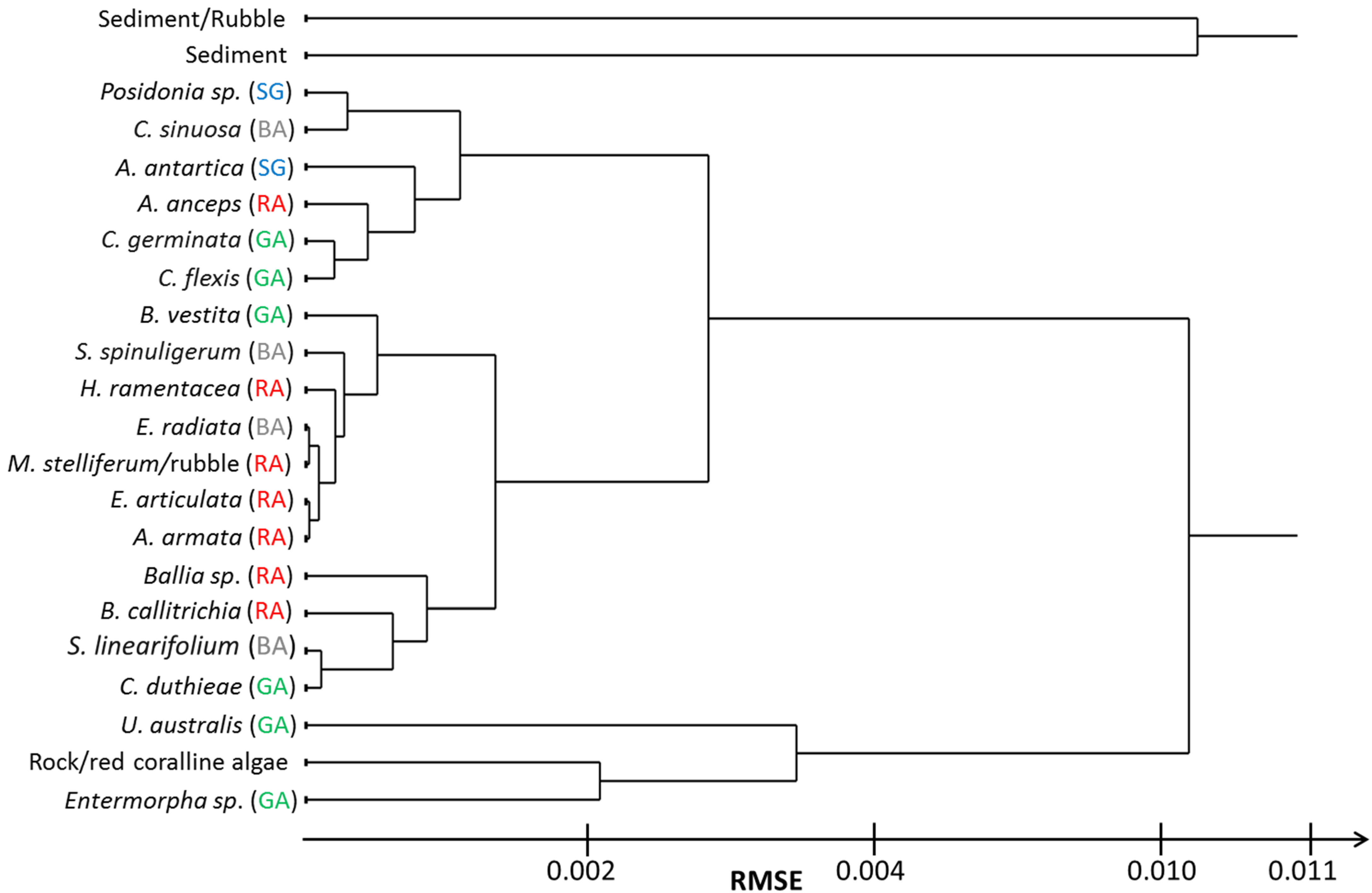
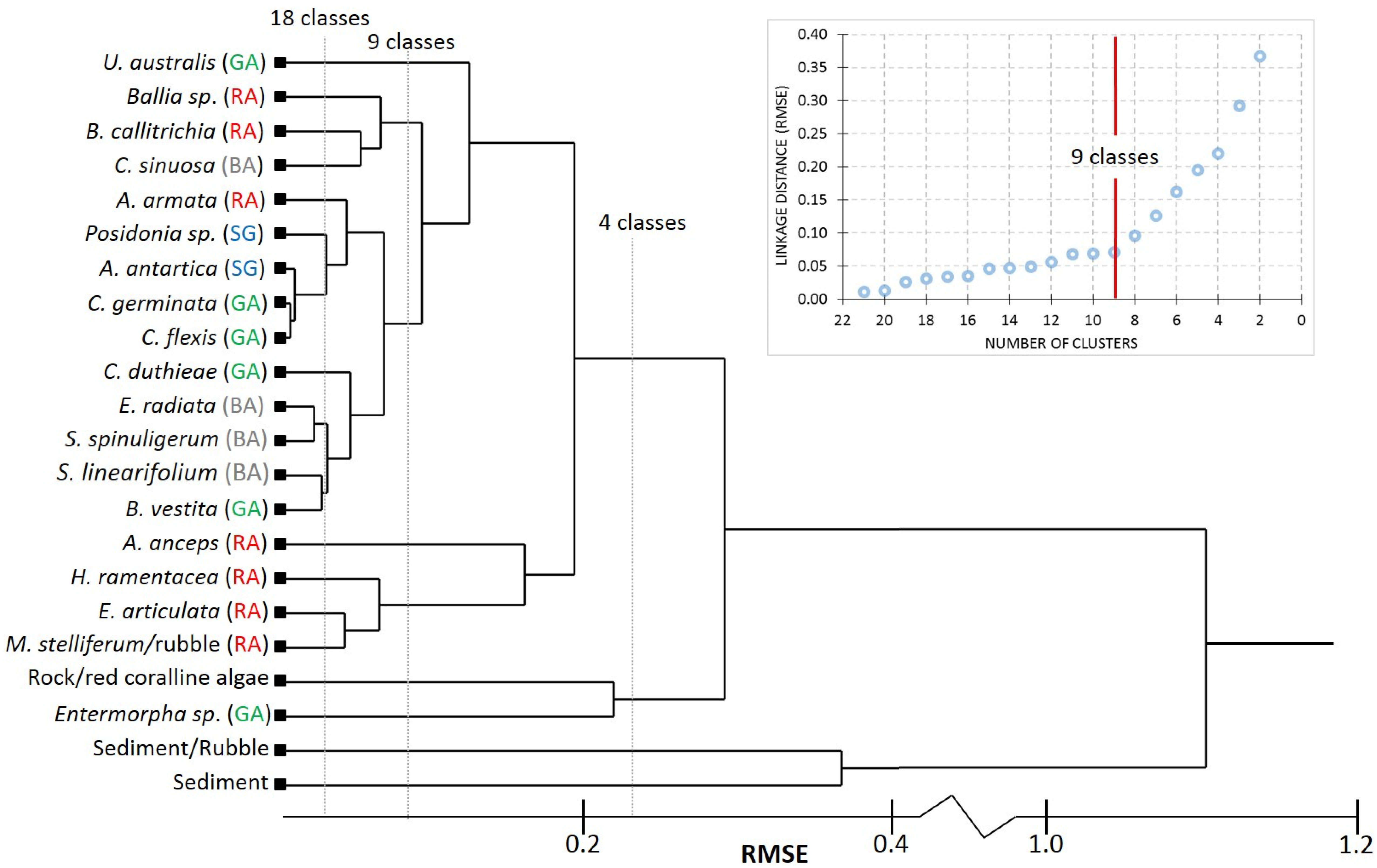
3.1. Hierarchical Clustering of Benthic Irradiance Reflectance Spectra

The HDC-derived dendrogram using the basic ρ_b spectra at HICO bands describes which benthic classes merge and the RMSE of that union (Figure 3). The respective dendrogram generated from the standard hierarchical clustering is presented in Figure 4. The RMSE refers to the spectral difference (in LD coordinates for the HDC algorithm) between one class mean and another, where the larger the value the larger the spectral difference. Based on the simulated spectral variability, occurring just below the air–water interface, the clustering output 18 classes for HICO (Figure 3) and HyMap (Figure 5) and 14 classes using WV2 bands (Figure 6). The clusters that were formed using HICO and HyMap bands were identical except that the merging of the clusters occurred at lower RMSE for HyMap (Figure 5). For example the merging of C. sinuosa with the cluster S. linearifolium/S. spinuligerum occurred at an RMSE of ~0.035 for HICO and ~0.032 for HyMap. This slight decrease in RMSE is likely due to the lower spectral resolution of the HyMap sensor or due to the lack of spectral bands below 450 nm (i.e., less spectral bands to facilitate separation). The dendrogram for HICO (Figure 3) and HyMap (Figure 5) show the formation of two green algae clusters (C. germinata/C. flexis and B. vestita/C. duthieae) and a brown algae cluster (C. sinuosa/S. linearifolium/S. spinuligerum) with the other benthic classes remaining optically separable. The dendrogram produced from the standard hierarchical clustering [45] (Figure 3) illustrates the potential indecision of what RMSE to cut the dendrogram and extract the relevant clusters. Here clustering continues to a single class with no indication of the optimum number of classes. At ~0.003 RMSE, 18 classes were extracted with the following clusters: (a) seagrass-green algae A. antartica/C. germinata/C. flexis; (b) mixed brown algae E. radiata/S. spinuligerum; and (c) brown-green algae S. linearifolium/B. vestita. A post clustering approach was utilized to estimate the appropriate number of classes from the standard hierarchical clustering (Figure 4). Here, nine classes was chosen as the optimum number, where the following general clusters remained: (a) two separate green algae species (Entromorpha sp. and U. australis); (b) two separate sediment classes (sediment/rubble and sediment); (c) mixed red/brown algae; (d) mixed brown, red, green algae and seagrass; and (e) a mixed red algae class. The number of classes selected by this post-clustering approach is much lower than that selected by the HDC. Moreover the HDC preferentially merges classes of the same genera first. For example the centroid hierarchical clustering merges the seagrass Posidonia sp. with the mixed C. germinata/C. flexis algae green class at the second iteration (Figure 4, RMSE ~0.0135), whereas the HDC considers these two classes optically distinct.

These two clustering algorithms generate different classes because the HDC first identifies pairs of classes with τ_m > 5% (the user defined threshold) and then merges the pair with the lowest RMSE (Mahalanobis distance in spectral space). The centroid based hierarchical clustering (Figure 4) instead merges the most similar class pairs regardless of whether their variance overlap or not. In other words a pair of classes may be grouped even if they could be considered optically distinct. An added advantage of the HDC is that the number of classes selected is imbedded inside the clustering, where the merging of clusters ceases when the variance overlap between groups is below a user defined threshold. Thus the criterion for stopping is statistically meaningful and aligns with the sensor and environmentally limited system of remote sensing as described and illustrated in Hedley et al. [26] (see Figure 1 in [26]). The user defined threshold describes the proportion of misclassification that a pair of classes should have before they are considered optically indistinguishable and hence merged. For example using HICO bands, the two classes C. germinata and C. flexis had a τ_m of 20%, i.e., 20% of the total spectra of these two classes were located in the overlap region and hence inseparable. Given that τ_m > 5% and proximity of the class means the HDC clustered these C. germinata and C. flexis after the second iteration.

The much lower spectral resolution and fewer wavebands of the WV2 sensor only facilitated the separation of 14 classes with the HDC. The dendrogram (Figure 6) shows the formation of the following clusters: (1) all the brown algae classes; (2) the green alga cluster Entermorpha sp./U. australis; (3) the mixed seagrass-green algae class of Posidonia sp./C. germinata/C. flexis/B. vestita; and (4) the red alga cluster E. articulata/M. stelliferum. Thus out of the seagrass species, only A. antartica was spectrally separable using WV2 bands. At the time of collection the seagrass Posidonia sp. samples were senescent and less spectrally distinct (using WV2 bands at least), which likely lead to its inclusion into the green algae cluster. Fyfe [50] compared the in-air reflectance of several unfouled and fouled seagrass species and showed that the latter had broader and less reflective peaks between 520–580 nm compared to the unfouled case. It is likely that this seagrass species can be optically separated if their reflectance spectra are collected during their growing season.

Figure 3. Dendrogram from the HDC of ρ_b spectra using HICO’s spectral bands. Here the iterative selection of eigenvectors chose the first six, which produced 18 classes.

Figure 3. Dendrogram from the HDC of ρ_b spectra using HICO’s spectral bands. Here the iterative selection of eigenvectors chose the first six, which produced 18 classes.

Figure 4. Dendrogram from the standard hierarchical clustering of ρ_b spectra using HICO’s spectral bands. The top right panel shows the linkage distance vs. number of clusters, where nine classes were selected as the optimal based on the location of the knee of the curve.

Figure 4. Dendrogram from the standard hierarchical clustering of ρ_b spectra using HICO’s spectral bands. The top right panel shows the linkage distance vs. number of clusters, where nine classes were selected as the optimal based on the location of the knee of the curve.

Figure 5. Dendrogram from the HDC of ρ_b spectra using HyMap spectral bands. The iterative selection of eigenvectors chose the first seven, which produced 18 classes.

Figure 5. Dendrogram from the HDC of ρ_b spectra using HyMap spectral bands. The iterative selection of eigenvectors chose the first seven, which produced 18 classes.

Figure 6. Dendrogram from the HDC of ρ_b spectra using WV2’s spectral bands. The iterative selection of eigenvectors chose the first four, which produced 14 classes.

Figure 6. Dendrogram from the HDC of ρ_b spectra using WV2’s spectral bands. The iterative selection of eigenvectors chose the first four, which produced 14 classes.

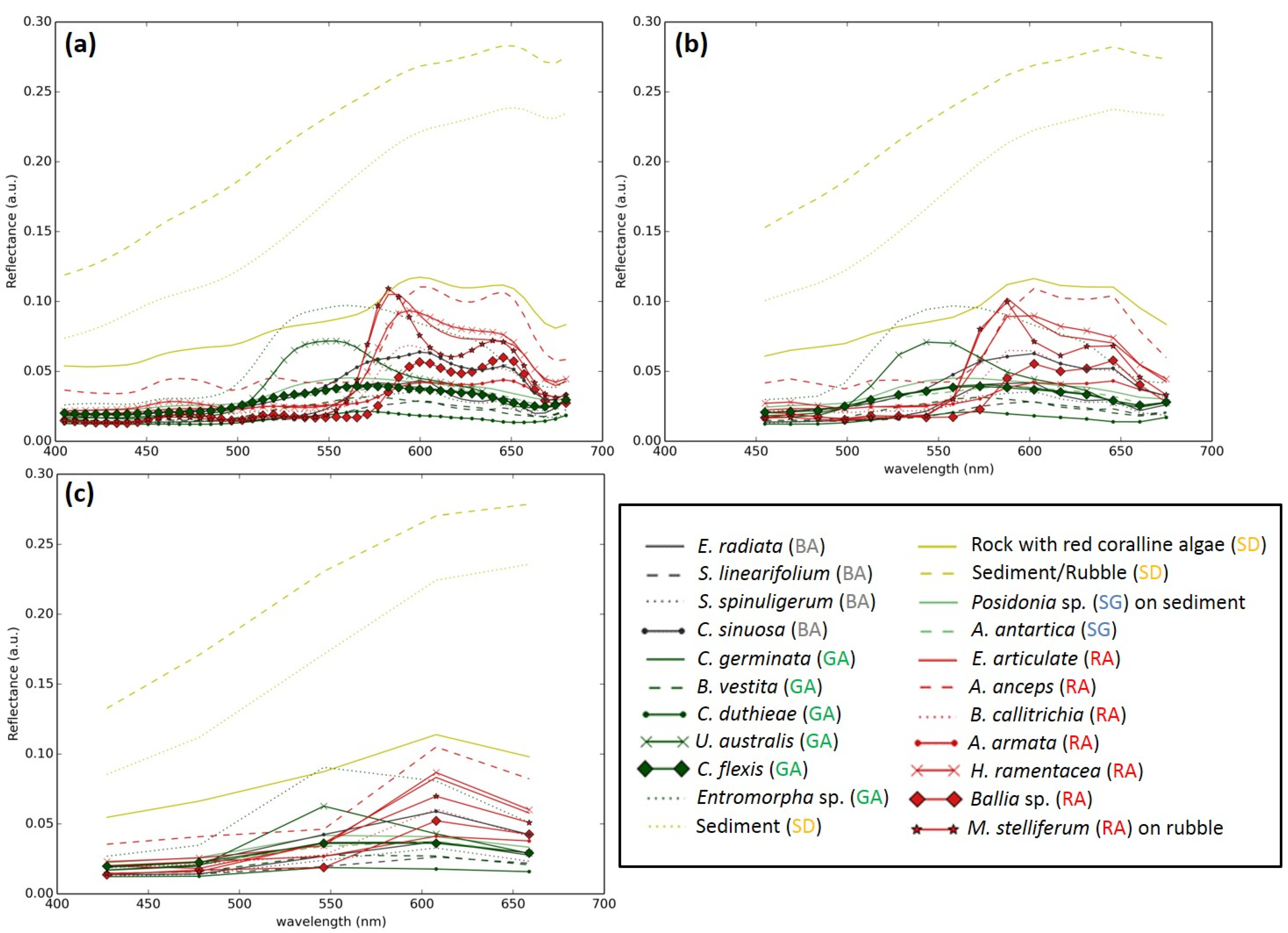
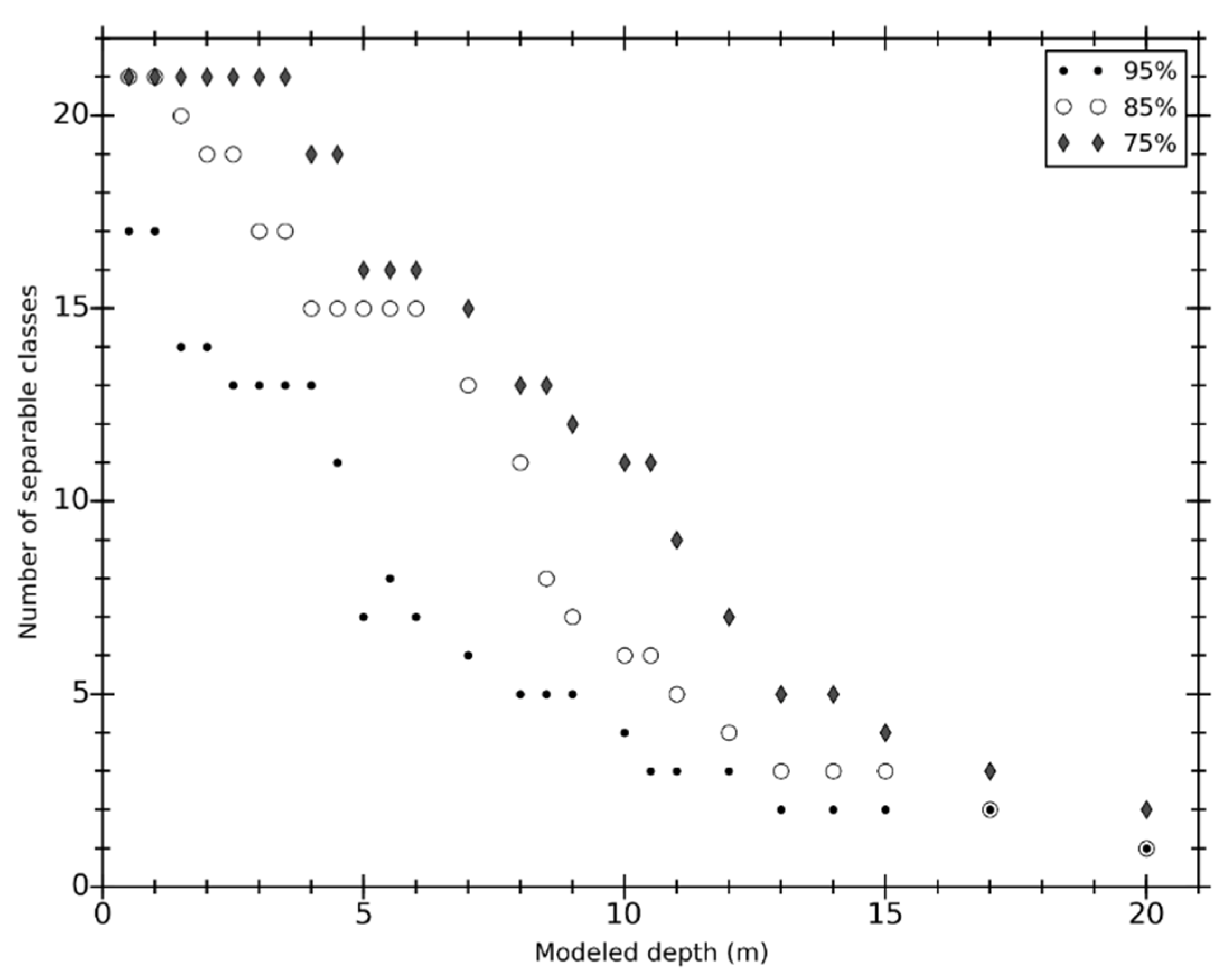
3.2. Water-Column Specific Benthic Spectral Libraries

Two spectrally distinct benthic classes remain at a modeled water depth and optical properties of 15.0 m, P = 0.05 m⁻¹, G = 0.10 m⁻¹ and X = 0.010 m⁻¹ using HICO bands (Figure 7). Here the HDC has merged all benthic vegetation species into a mixed vegetation class and merged the remaining two sediment classes. Thus at this water column optical property and depth it is not possible to distinguish between any of the initial benthic vegetation species above the total system noise, and only a bright (i.e., sediment) and dark (i.e., vegetation) substrate can be distinguished, assuming completely filled pixels of each type. Figure 7 shows the possibility of determining a priori which benthic classes are separable in a single image pixel at a fixed depth and optical property. Thus for an image with varying depths and water column optical properties the HDC clustering will need to be applied per-pixel. Physics-based inversion methods can be used to derive the depth and water column optical properties as will be discussed in Section 3.4.

The decrease in the number of optically separable benthic classes for increasing depth and water column turbidity at HICO, HyMap and WV2 bands was quantified with the HDC clustering (Figure8). Clear to turbid water columns (Figure 8, water types 1 and 4 respectively) were modeled to assess their impact on benthic class optical separation. For a given water clarity the number of optically distinguishable benthic classes decreased in a near exponential manner with increasing depth, as has been described in the literature [26,48]. Increasing the water turbidity also reduces the number of separable classes dramatically with increasing depth. With HICO spectral bands, 13 classes can be optically distinguished at 5 m depth for water type 1 (48 m Secchi depth, Figure 8a), whereas only 11, 6 and 2 classes are separable for water types 2, 3 and 4 (Secchi depths of 13, 6.2 and 2 m) respectively at that depth. The water column saturation point, that is, where the water column contributes to nearly all of the water leaving radiance, is located when none of the benthic classes can be distinguished (i.e., number of classes = 1). For water types 2, 3 and 4 these occur at depths 20 m, 12 m and 5.5 m respectively using HICO bands.

Decreasing the number of spectral bands also increases the slope of the exponential curve as illustrated when comparing Figure 8a (HICO) and Figure 8c (WV2). For water type 3 at 3 m depth the HICO, HyMap and WV2 wavebands, according to the HDC, can distinguish 12, 11 and 5 classes respectively. Increasing the depth to 5 m reduced the number of classes to 6, 6 and 3 respectively. For depths less than the water column saturation point, the five WV2 bands between 400 and 680 nm can generally separate half as many benthic classes as HICO. Based on the modeling shown in Figure 8 and a comparison between the exponential slopes, there appears to be minor differences in the number of classes distinguishable at depth between HICO and HyMap wavebands. In this analysis, wavelengths between 400 and 680 nm were used which reduced the number of bands to 49 and 16 for HICO and HyMap respectively. This may seem like a large reduction of wavebands without greatly affecting the benthic separability. We should note that unlike HICO, HyMap does not have bands below 450 nm [51], hence both sensors have wavebands that emphasize the spectral differences between the benthic classes analyzed. The literature has shown that specific wavelength ranges predominantly within 520–680 nm are useful for identifying substrate types, such as healthy coral, bleached coral, seagrass, sand and algae [34,39,50,52,53]. Therefore, it is likely that the difference in bandwidth is the cause where the spectral resolution of HICO and HyMap are 5.7 and 15 nm [51] respectively. This is in line with what Hochberg and Atkinson [24] showed where the separation of coral, algae and sand using LDA were nearly identical for spectra at 10, 5.5 and 1 nm spectral resolutions.

Figure 7. Dendrogram from the HDC of modeled r_rs spectra using HICO’s spectral bands. The water column was modeled with depth 15 m and P = 0.05, G = 0.1 and X = 0.010 m⁻¹. Here the iterative eigenvector selection chose only one eigenvector.

Figure 7. Dendrogram from the HDC of modeled r_rs spectra using HICO’s spectral bands. The water column was modeled with depth 15 m and P = 0.05, G = 0.1 and X = 0.010 m⁻¹. Here the iterative eigenvector selection chose only one eigenvector.

Figure 8. Number of optically separable classes vs. depth using the spectral bands and resolutions for (a) HICO; (b) HyMap; and (c) WV2. Four water-columns were modeled with varying water turbidity representing very clear to turbid waters. The exponential curves were derived through a least squares fit.

Figure 8. Number of optically separable classes vs. depth using the spectral bands and resolutions for (a) HICO; (b) HyMap; and (c) WV2. Four water-columns were modeled with varying water turbidity representing very clear to turbid waters. The exponential curves were derived through a least squares fit.

The number of classes within a spectral library can be stratified with depth, for instance using water type 1, the spectral library for WV2 (Figure 8c) has the same number of classes from 5 m to 15 m. Stratification in the number of classes is expected as they are integer values and hence more emphasized in slowly decreasing curves and less observed in areas of rapid change (e.g., 0–3 m depth of Figure 8b for water type 3). Analyses of the spectral libraries from all three sensors within the stratified regions of a given water type indicate that at >5 m the output classes produced are identical though subtle differences exist in the RMSE of when classes merge. At shallower depths, however, the spectral libraries in the stratified regions have minor differences in the classes that merge and thus in the output classes. For HICO spectral bands 13 classes were generated in the stratified region between 3 and 6 m depth with water type 1. The spectral libraries at 3 and 4 m are identical as are the spectral libraries at 5 and 6 m (Table 3). Between these two sets of spectral libraries the following differences occur: (1) the brown alga E. radiata and C. sinusoa from the mixed vegetation class (at 3 m) split to form an individual mixed brown algae class; and (2) the union of E. articulata and M. stelliferum (Table 3).

Table 3. The classes from the HICO spectral libraries at depths 3–6 m using water column optical properties of P = 0.01 m⁻¹, G = 0.01 m⁻¹, and X = 0.001 m⁻¹. The superscripts represent the number of species that form that cluster, for example mixed brown algae⁴ means that four brown algae species were merged to form one mixed brown algae class. The spectral libraries at 5 and 6 m depth are identical.

Table 3. The classes from the HICO spectral libraries at depths 3–6 m using water column optical properties of P = 0.01 m⁻¹, G = 0.01 m⁻¹, and X = 0.001 m⁻¹. The superscripts represent the number of species that form that cluster, for example mixed brown algae⁴ means that four brown algae species were merged to form one mixed brown algae class. The spectral libraries at 5 and 6 m depth are identical.

The classes from the HyMap spectral libraries for depths 3 to 6 m with water type 1 are given in Table 4. A stratified region (Figure 8b) is formed in this depth range and water type, where 12 classes are optically separable at 3, 5 and 6 m depth. At 3 m depth four species of brown algae merge to form one cluster, however at 4, 5 and 6 m two of those brown algae species (E. radiata and C. sinusoa) form a separate mixed class and the other two merge into a mixed brown algae/green algae/seagrass class (Table 4). Other differences include: (1) the separation of the Sediment-Rubble/Sediment class (3 and 4 m) to their individual class at 5 and 6 m; and (2) the union of the green alga Entermorpha sp. and U. australis at >3 m depth. Some clusters are consistently generated within this depth range which include Rock-red coralline algae and six red algae classes E. articulata/M. stelliferum, Ballia sp., H. ramentacea; A. armata; B. callitrichia, and A. anceps. Indeed each spectral library between 3 and 6 m has six red algae classes, >1 sediment class, >1 green algae class and a mixed vegetation class. At 4 m depth the HDC procedure generated 11 classes using three eigenvectors, analysis has shown that using six eigenvectors facilitates the separation of 12 classes identical to that produced at 5 and 6 m (Table 4). Here six eigenvectors were not used because the fourth and fifth eigenvectors did not increase the number of clusters generated and thus the iterative eigenvector selection procedure chose the first three. Like for HICO (Table 3) there are minor differences between spectral libraries in these stratified regions, as such we propose the use of a single spectral library for such regions.

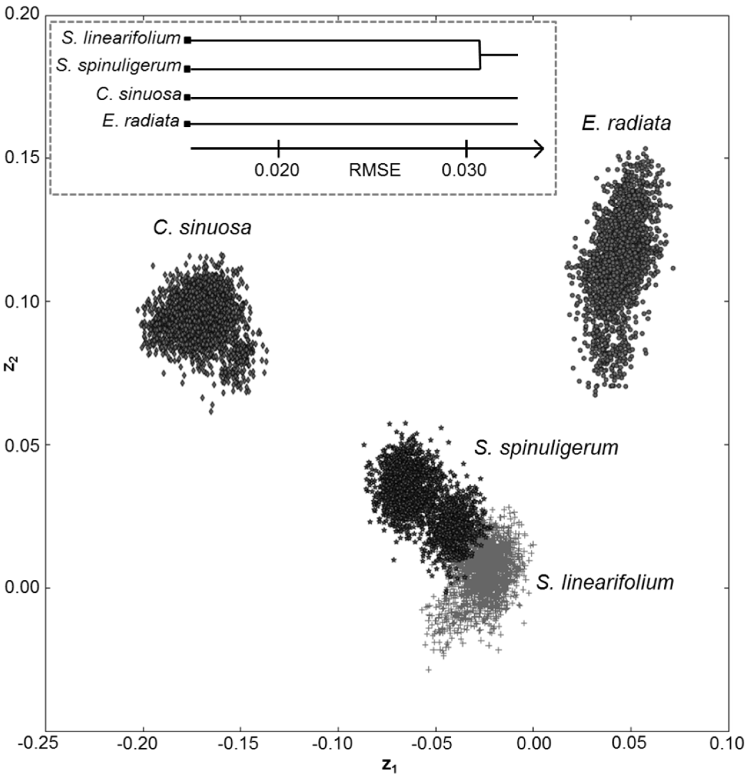
3.3. Resolving Seagrass Species from Algae

An important ecological application of optical remote sensing is mapping seagrass meadows [54]. Using the HDC algorithm, we consider the clustering accuracy, sensor spectral resolution, water column depth and optical properties that enable the optical distinction of the seagrass species A. antartica from green and brown alga. Figure 9 shows the modeled depth at which we can no longer resolve A. antartica from the green algae species (Table 2) for clear to turbid water clarities (water types 1 to 4 respectively) using the different sensors. Thus for HICO bands A. antartica is optically distinguishable from green algae to a depth of approximately 4.25 m at 90% clustering accuracy for a clear water column (water type 1, Figure 9a). Beyond this depth at 90% accuracy A. antartica cannot be spectrally distinguished. Note that the results for WV2 in Figure 9c relates to the ability of distinguishing A. antartica from the Posidonia sp./green algae cluster, as the latter seagrass species could not be resolved using bottom reflectances (Figure 6).

For a given water type, decreasing the clustering accuracy enables the ability to spectrally resolve seagrass from green algae to greater depths. The reason being that the HDC allows for greater misclassification proportion between pairs of classes before they are considered “indistinguishable”. For example, using HyMap bands A. antartica can be distinguished at 2.5 and 3.75 m for water type 2 at 85% and 75% clustering accuracies respectively (Figure 9b). Therefore if the user desires the ability to map A. antartica up to a depth of 4 m with HyMap, then 75% clustering accuracy should be used for water columns with Secchi depths greater than 13 m. A reduction of the water clarity also decreases the ability to resolve species at depth, as observed by the ability of WV2 to distinguish A. antartica to 2 m and 0.75 m for water types with Secchi depths 48 and 2 m (Figure 9c) respectively at 80% accuracy. Therefore as the modeled water depth or turbidity is increased the distances between classes decreases such that neighboring classes experience more overlap [26]. Hence a greater τ_m accounts for the decrease in the inter-class distance, where classes are considered optically distinct despite their increase in overlap. We have low confidence for results that used clustering accuracies less than 70% as, for example, HyMap bands can distinguish A. antartica to 2.25 m for water type 4 (Figure 9b) that has an estimated Secchi depth of 2 m.

Figure 9. The estimated modeled depth (m) at which A. antartica can no longer be distinguished from green algae at various clustering accuracies for (a) HICO; (b) HyMap and (c) WV2 wavebands. Clear (water type 1) to turbid (water type 4) water clarities were modeled. The depths given here are estimates as the clustering at every 0.25 m depth increment were analyzed.

Figure 9. The estimated modeled depth (m) at which A. antartica can no longer be distinguished from green algae at various clustering accuracies for (a) HICO; (b) HyMap and (c) WV2 wavebands. Clear (water type 1) to turbid (water type 4) water clarities were modeled. The depths given here are estimates as the clustering at every 0.25 m depth increment were analyzed.

The advantage of using hyperspectral sensors is clearly demonstrated in Figure 9, where HICO and HyMap have the ability to resolve seagrass from green algae to much greater depths for a given clustering accuracy and water clarity compared to WV2. Indeed at 85% clustering accuracy, HICO and HyMap spectral bands can distinguish A. antartica to an estimated depth of 6.5 and 3.75 m respectively for water type 1 (48 m Secchi Depth), whilst WV2 can only resolve it to a depth of 1.5 m. On average HICO bands can detect A. antartica to depths 2.7 times greater than WV2 bands across the clustering accuracies and water types. In most conditions analyzed there is close similarity in the depth limits at which A. antartica can be resolved using HICO and HyMap bands, where on average HICO can detect this species to depths 1.2 times greater than HyMap.

Table 4. The classes from the HyMap spectral libraries at depths 3–6 m using water column optical properties of P = 0.01 m⁻¹, G = 0.01 m⁻¹, and X = 0.001 m⁻¹. The superscripts represent the number of species that form that cluster, for example mixed brown algae⁴ means that four brown algae species were merged to form one mixed brown algae class. The spectral libraries at 5 and 6 m depth are identical.

* Six eigenvectors generated 12 classes identical to those at 5 and 6 m.

Table 4. The classes from the HyMap spectral libraries at depths 3–6 m using water column optical properties of P = 0.01 m⁻¹, G = 0.01 m⁻¹, and X = 0.001 m⁻¹. The superscripts represent the number of species that form that cluster, for example mixed brown algae⁴ means that four brown algae species were merged to form one mixed brown algae class. The spectral libraries at 5 and 6 m depth are identical.

* Six eigenvectors generated 12 classes identical to those at 5 and 6 m.

The ability to spectrally resolve mixed seagrass/green algae from brown algae was analyzed for the same conditions presented in Figure 9. However, a direct comparison between seagrass and brown algae was not possible for HICO, HyMap and WV2 at any of the water column conditions presented. The reason being that Posidonia sp. and A. antartica both merge with a mixed green algae class. This seagrass/green algae mix then clusters with a mixed brown algae class at deeper depths. The distinction between mixed seagrass/green algae and brown algae (effectively between green and brown colored benthic species) follows the same trend as that presented in Figure 9 expect that they can be distinguished to much deeper depths.

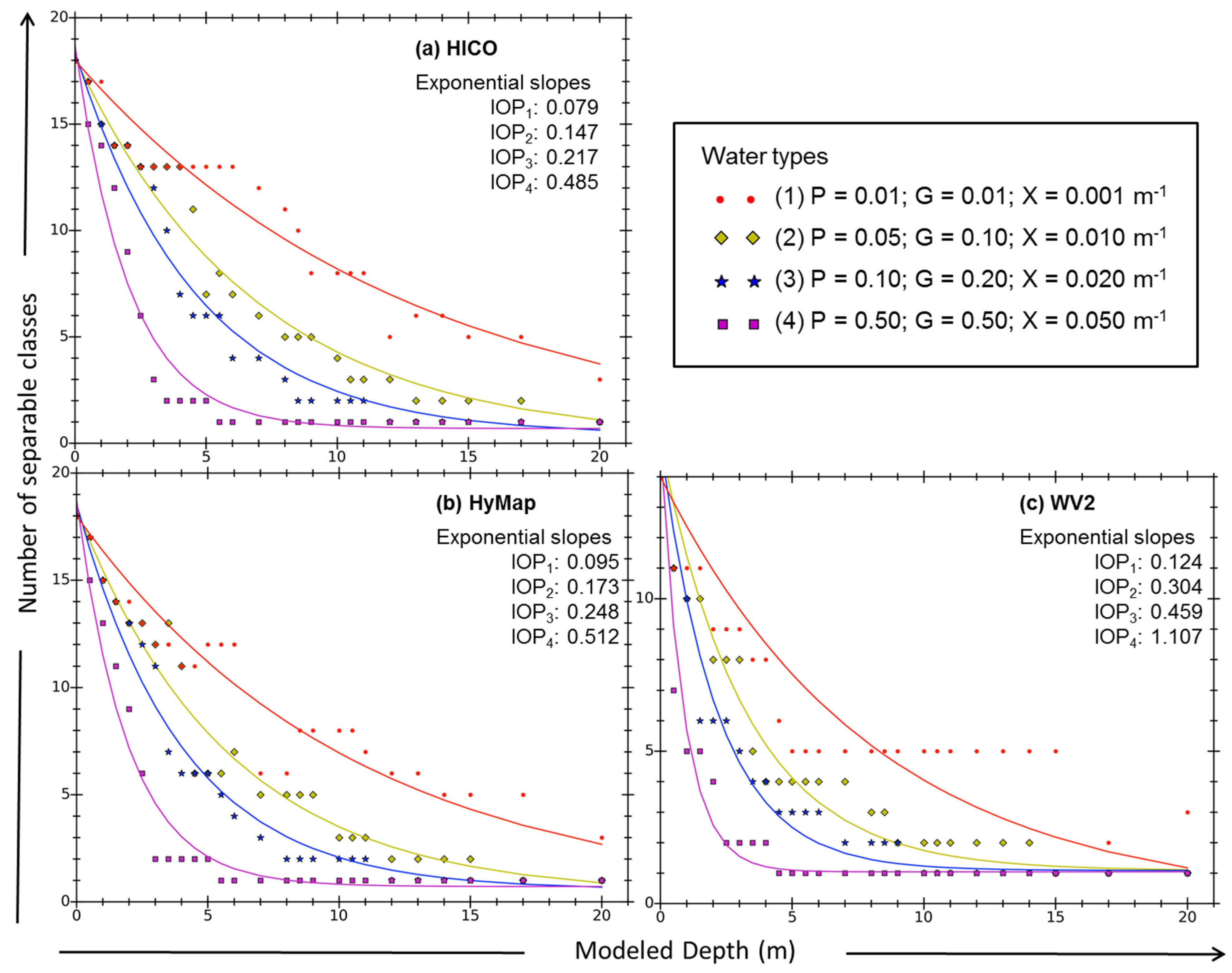
3.4. Implications to Shallow Water Habitat Mapping

Modeling for a variety of water turbidities and depth as displayed in Figure 8 enables predictions on the number and type of benthic classes that can be expected from a hyperspectral or multispectral image at a constant clustering accuracy. The level of accuracy can be changed according to the needs of the user or application with corresponding changes to the number and type of benthic classes defined by the HDC. Figure 10 illustrates that the number of optically separable classes increases as the clustering accuracy decreases for a constant set of water column optical properties at HICO wavebands. These results are similar to those produced by Andrefouet et al. [1] where the thematic accuracy decreased with increasing number of habitat classes used in the benthic classification scheme. Although thematic and clustering accuracy are applied in different contexts, Figure 8 does imply that if a benthic habitat map at a constant classification accuracy is required, then the number of classes used in the classification scheme must change with the range of depths and water column optical properties within an image. Prior knowledge of the depth and optical properties in a given scene therefore becomes a requisite in applying the HDC algorithm. Note the depth, P, G, and X can be determined by applying a shallow water inversion model for sensors with enough spectral bands in the visible [16,17]. Here the full benthic spectral library could be used solely to optimize these parameters.

Figure 10. Number of optically separable classes vs. depth at three different clustering accuracies using the spectral bands and resolutions for HICO. The water column was modeled with P = 0.05, G = 0.1 and X = 0.010 m⁻¹.

Figure 10. Number of optically separable classes vs. depth at three different clustering accuracies using the spectral bands and resolutions for HICO. The water column was modeled with P = 0.05, G = 0.1 and X = 0.010 m⁻¹.

Benthic classifications of remotely sensed imagery using physics-based inversion models to date have used a spectral library of representative benthic species (fine descriptive resolution, see Dekker et al. [20]). Depending on the shallow water model used, the inversion process iterates through unique combinations of benthic mixtures and optimizes for their fractional coverage, water column optical properties and depth. The benthic combination and fractional coverage that generated the best fit to the input reflectance are assigned. Therefore distinct benthic species would be assigned to image pixels at any given depth and water column optical property, no matter if it were unlikely to distinguish one benthic species from another.

The research presented here indicates that this type of benthic classification may not be appropriate, particularly when mapping regions of varying water depths or when propagating sensor and environmental noise in the inversion scheme [41,42,44,55]. This can be illustrated by the dendrogram presented in Figure 7, where the at-surface spectral differences between the benthic vegetation species do not make observable differences to r_rs above the total system noise at the depth and P, G and X modeled. Clearly if a spectral library consisting of the initial 22 benthic classes were used for an inversion of say a pixel having 100% coverage of E. radiata with P, G, X and depth used in Figure 7; then accordingly a shallow water inversion model would likely not be able to distinguish the forward modeled r_rs derived from E. radiata from any other benthic vegetation species when NEΔr_rs is incorporated. In this situation it is likely that equal probability of assignment across the benthic vegetation classes will result. This was illustrated in Figure 5 by Hedley et al. [42] where the uncertainty of the bottom type increased with depth and increasing number of endmembers in the spectral library. Furthermore, the assignment of a specific benthic species (even correctly identified E. radiata) cannot be made with sufficient certainty, and a classification assignment of “mixed vegetation” would be more appropriate for these optical properties and depth. In fact such a class name would convey that level of uncertainty and lack of spectral separability. Indeed, analysis of HDC-derived output classes has showed that as the water column becomes more turbid or deeper, the ability to distinguish distinct benthic species is lost, where resultant classes consist of mixed clusters. Again in these situations, assigning the appropriate mixed cluster would help convey the level of certainty and optical separability into the classification scheme.

Presently the HDC algorithm assumes 100% substrate coverage of a pixel and as a post-inversion tool would be suited for high spatial resolution image data. In addition, its application would be more appropriate towards constraining the benthic classification of the HOPE inversion model [16], if the endmembers of a high descriptive resolution spectral library were cycled through during the optimization process. Note that the HOPE model considers one substrate endmember rather than a linear mixture of two [18] or three [17]. The requirement of moderate to high spatial resolution image data does limit the applicability of the HDC algorithm as a post-inversion tool to mostly airborne sensors such as AISA Eagle, HyVista’s HyMap, CASI-2, AVIRIS and Ocean PHILLS. From the current and planned satellite sensors, WV2, Sentinel-2 and VENμS SSC [56] possess high spatial resolution (≤10 m) and enough spectral bands in the visible domain to facilitate optimization using current shallow water inversion models (e.g., [42,57]).

Analysis has showed that the HDC-derived water column specific libraries are sensor and scene specific. Sensor specific because the number and type of HDC-derived benthic classes depend on the sensor’s spectral resolution and signal to noise ratio. Scene specific because: (1) the environmental noise in the imagery, such as sunglint which even if corrected [58] leaves residual spatial noise; and (2) The number and type of output classes are dependent on the representative benthic species present. The latter is implied by the clustering of the seagrass Posidonia sp. and the green algae C. germinata, C. flexis and B. vestita at WV2 bands (Figure 6). If none of the green algae species were present in the scene then Posidonia sp. would be spectrally distinct, and would lead to different benthic class mixtures.

As the clustering is based on LD coordinates the ability to distinguish individual classes potentially decreases when the number of initial classes increase. This is illustrated in Figure 11, which shows the LD coordinates of the four brown algae E. radiata, S. linearifolium, S. spinuligerum and C. sinuosa. Three clusters resulted when the ρ_b spectra (at HICO bands) of these four brown algae species were passed through the HDC algorithm (see Figure 11). Recall that two brown algae clusters were considered distinct (S. linearifolium/S. spinuligerum/C. sinuosa and E. radiata) when the initial spectral library of 22 classes where passed through the HDC (see dendrogram in Figure 3). The reason for this is that the LDA seeks a projection that maximizes the distance between classes whilst minimizing the within-class variance [59,60]. Thus in the case of Figure 11, an optimal projection was found that enabled the distinction of three brown algae clusters. These results imply that only a minimal set of initial benthic classes should be used in the clustering.

Figure 11. LD coordinates of the four brown algae species using HICO wavebands. The HDC-derived dendrogram is shown on the top left corner. Here one eigenvector (z₁) allowed the optimal distinction of the following three clusters: (1) S. linearifolium/S. spinuligerum; (2) E. radiata, and (3) C. sinuosa.

Figure 11. LD coordinates of the four brown algae species using HICO wavebands. The HDC-derived dendrogram is shown on the top left corner. Here one eigenvector (z₁) allowed the optimal distinction of the following three clusters: (1) S. linearifolium/S. spinuligerum; (2) E. radiata, and (3) C. sinuosa.

Although a sensor’s spectral characteristics, total system noise and water column attenuation affect substrate separability; spatial resolution, not accounted by the HDC algorithm, also plays a significant role. Particularly since coastal and coral reefs can be spatially heterogeneous, where a diverse array of spectrally distinct substrates can occur at sub-meter scales [55]. Previous research involving thematic mapping and Object-Based Image Analysis of coral reefs has shown improved benthic classification using imaging platforms with high spatial resolution (<10 m) compared to those with moderate resolution (30 m) [61]. Thus although a sensor, such as HICO, with high spectral resolution can spectrally discriminate between many benthos to deeper depths, its spatial resolution (~90 m) will significantly affect the ability to resolve individual substrates compared to HyMap or even WV2 with resolutions less than 10 m. For moderate spatial resolution sensors broad classification of pixels into key substrate components would be a more feasible approach (e.g., [17,62]).

As a final note, a sensor’s radiometric calibration and the atmospheric correction can significantly affect the accuracy of the retrievals from inversion models [20], and hence on subsequent results from the HDC-algorithm as a post-inversion tool. Image pre-processing steps have been used, prior to shallow water inversion models, to minimize the effect of residual under- or over-atmospheric correction [17,63]. In Klonowski et al. [17] the R_rs of an image were vertically shifted to make R_rs(750) = 0, this approach was later modified where the R_rs were subtracted by the median value between 650 and 800 nm [20]. In Lee et al. [63] the R_rs were adjusted by setting the R_rs(750) to a value computed from an empirical relationship. These approaches are therefore useful if the atmospheric parameters were assumed constant for an image and the atmospheric correction produced a systematic offset. Atmospheric correction that deduce atmospheric parameters per-pixel can potentially use different aerosol models in an image and thereby cause variation in the spectral shape of the derived R_rs. If imprecise the pre-processing steps will not be able to account for an incorrect spectral shape of the R_rs. Radiometric sensor calibration can also significantly affect both the shape and offset of sensor-derived R_rs. Indeed, Lewis et al. [64] showed substantial improvement in match ups between in situ and HICO-derived water leaving radiance after vicarious calibration. Minimizing errors from calibration and atmospheric correction is particularly crucial over dark targets such as deep water or submerged aquatic vegetation. This is due to a reduced signal-to-noise ratio and where a higher proportion of the at-sensor radiance is contaminated by the atmospheric path radiance compared to bright shallow targets. Hence small errors in the calibration or deviations of the actual atmospheric parameters compared to what is used during atmospheric correction can produce negative reflectances [65,66,67]. Improvements to a sensor’s SNR, accurate calibration and atmospheric correction will lead to improved benthic classification from shallow water inversion models. We note that the use of the HDC algorithm to examine the ability of spectrally resolving a set of representative substrates for various environmental conditions takes into account noise introduced from inaccurate atmospheric or sunglint correction.

4. Conclusions

We have presented an agglomerative hierarchical clustering using linear discriminant coordinates (HDC), which when used on a spectral library of benthic endmembers outputs those classes that are optically distinguishable above the total system’s variability. The HDC clustering differs from other hierarchical clustering schemes by the inclusion of the system’s total variability onto each data point and the clustering based on pairwise distance and misclassification proportions. The iterative merging of classes in the HDC ceases when the remaining classes have a misclassification rate below a user specified threshold. Thus the user does not need to decide beforehand or post-clustering the number of classes to output—a common problem faced in the application of clustering procedures. Rather the total system’s variability controls this outcome where a noisier system would lead to fewer output classes for a given misclassification threshold and vice-versa. In the context of benthic classification from shallow water remote sensing, variability arises from the sensor and environment (imperfect atmospheric, sunglint and air–water interface corrections) and the spectral variability observed within a given benthic species. Both sources degrade the spectral separability between benthic classes.

The HDC was applied to a set of measured reflectance spectra of 22 benthic classes collected from the Point Peron study site, Western Australia. This initial spectral library contained the sub-local scale spectral variability of each benthic class and with the addition of sensor and environmental noise taken from a HICO image, accounted for the total system’s variability. Analysis of the clustering on datasets convolved to the wavebands of WV2, HyVista’s HyMap and HICO sensors showed a reduction in spectral resolution reduced the spectral separability between classes and hence reduced the number of distinct classes. For instance, at WV2 and HICO wavebands 14 and 18 classes were spectrally separable just below the water’s surface respectively, from the initial 22. Dendrograms from the HDC have showed that benthic species from a given genera preferentially merge first before clustering with species of other genera.

Depth and water column turbidity have been demonstrated in the literature as the most influential factor inhibiting benthic classification, where fewer classes are optically separable with increasing depth and/or turbidity. Using the measured benthic reflectance spectra, a shallow water forward model was used to simulate the water-leaving subsurface reflectance at any specified depth and water column optical property. Combined with the HDC, depth and water column specific spectral libraries were generated and subsequent analysis have quantified that the number of benthic classes decreases with increasing depth and water column turbidity at a constant clustering accuracy. Furthermore, the clustering analysis identifies those benthic classes that merge as a consequence of water column attenuation and the total system’s noise.

If the irradiance reflectance spectra of the representative benthos in a scene of interest are known, then the HDC algorithm offers the ability to explore the potential of benthic classification from shallow water remote sensing, where the number and type of classes can be quantified for any given sensor, clustering accuracy, water column optical property and depth. From a management perspective, the HDC can be used to pre-determine which sensor to use so that the mapping requirements match the expected outcomes from the resultant benthic classification map. This was illustrated through the analysis of conditions that include clustering accuracy, water clarity and depth and spectral resolution that enable A. antartica to be spectrally resolved from benthic algae. Such an analysis can aid in an assessment of the feasibility of detecting phase shifts in seagrass meadows, for example, from a variety of sensors; but does not incorporate the effect of spatial resolution, which can decrease spectral distinctions. In situations where local knowledge of the spectral library is absent then the algorithm presented here cannot be applied, as the derived class names are scene specific.

Further research includes the validation of the HDC algorithm with vertical profiling optical measurements and above water radiometry. Such studies would include a comparative analysis of the clustering algorithm to optical measurement based cluster dendrograms using the rand index [68] or cophenetic correlation [69], in an analogous manner to Torrecilla et al. [47]. Further development includes the application of the HDC-derived spectral libraries into physics-based shallow water inversion models. The purpose of which would be to obtain a benthic classification map with more appropriate class names that help convey the level of certainty and optical separability. It is likely that the resultant benthic classification map will be depth dependent (and hence layered), as the class names (and numbers) change with depth. Change detection is also an avenue of future research, particularly in assessing the amount of temporal change of a benthic species when it is not spectrally distinct at depth. In other words, assessing which benthic species/clusters we can detect temporal changes in. Mixed benthic assemblages typically occur at spatial resolutions greater than 2 m, how this affects benthic classification using HDC-derived spectral libraries should be investigated.

References

1. Andrefouet, S.; Kramer, P.; Torres-Pulliza, D.; Joyce, K.E.; Hochberg, E.J.; Garcia-Perez, R.; Mumby, P.J.; Riegl, B.; Yamano, H.; White, W.H.; et al. Multi-site evaluation of IKONOS data for classification of tropical coral reef environments. Remote Sens. Environ. 2003, 88, 128–143. [Google Scholar]
2. Mumby, P.J.; Harborne, A.R. Development of a systematic classification scheme of marine habitats to facilitate regional management and mapping of Caribbean coral reefs. Biol. Conserv. 1999, 88, 155–163. [Google Scholar] [CrossRef]
3. Mumby, P.J.; Green, E.P.; Edwards, A.J.; Clark, C.D. Coral reef habitat mapping: How much detail can remote sensing provide. Mar. Biol. 1997, 130, 193–202. [Google Scholar] [CrossRef]
4. Mumby, P.J.; Clark, C.D.; Green, E.P.; Edwards, A.J. Benefits of water column correction and contextual editing for mapping coral reefs. Int. J. Remote Sens. 1998, 19, 203–210. [Google Scholar] [CrossRef]
5. Mumby, P.J.; Green, E.P.; Clark, C.D.; Edwards, A.J. Digital analysis of multispectral airborne imagery of coral reefs. Coral Reefs 1998, 17, 59–69. [Google Scholar] [CrossRef]
6. Mumby, P.J.; Hedley, J.D.; Chisholm, J.R.M.; Clark, C.D.; Ripley, H.; Jaubert, J. The cover of living and dead corals from airborne remote sensing. Coral Reefs 2004, 23, 171–183. [Google Scholar] [CrossRef]
7. Vahtmae, E.; Kutser, T. Mapping bottom type and water depth in shallow coastal waters with satellite remote sensing. J. Coast. Res. 2007, S50, 185–189. [Google Scholar]
8. Mumby, P.J.; Edwards, A.J. Mapping marine environments with IKONOS imagery: Enhanced spatial resolution can deliver greater thematic accuracy. Remote Sens. Environ. 2002, 82, 248–257. [Google Scholar] [CrossRef]
9. Vahtmae, E.; Kutser, T.; Kotta, J.; Parnoja, M. Detecting patterns and changes in a complex benthic environment of the Baltic Sea. J. Appl. Remote Sens. 2011, 5, 053559. [Google Scholar] [CrossRef]
10. Purkis, S.; Kenter, J.A.M.; Oikonomou, E.K.; Robinson, I.S. High-resolution ground verification, cluster analysis and optical model of reef substrate coverage on Landsat TM imagery (Red Sea, Egypt). Int. J. Remote Sens. 2002, 23, 1677–1698. [Google Scholar] [CrossRef]
11. Dekker, A.G.; Brando, V.E.; Anstee, J.M. Retrospective seagrass change detection in a shallow coastal tidal Australian lake. Remote Sens. Environ. 2005, 97, 415–433. [Google Scholar] [CrossRef]
12. Gullstrom, M.; Lunden, B.; Bodin, M.; Kangwe, J.; Ohman, M.C.; Mtolera, M.S.P.; Bjork, M. Assessment of changes in the seagrass-dominated submerged vegetation of tropical Chwaka Bay (Zanzibar) using satellite remote sensing. Estuar. Coast. Shelf Sci. 2006, 67, 399–408. [Google Scholar] [CrossRef]
13. Hedley, J.D.; Mumby, P.J.; Joyce, K.E.; Phinn, S.R. Spectral unmixing of coral reef benthos under ideal conditions. Coral Reefs 2004, 23, 60–73. [Google Scholar] [CrossRef]
14. Mobley, C.D.; Sundman, L.K.; Davis, C.O.; Bowles, J.H.; Downes, T.V.; Leathers, R.A.; Montes, M.J.; Bissett, W.P.; Kohler, D.D.R.; Reid, R.P.; et al. Interpretation of hyperspectral remote-sensing imagery by spectrum matching and look-up-tables. Appl. Opt. 2005, 44, 3576–3592. [Google Scholar] [CrossRef] [PubMed]
15. Hedley, J.; Roelfsema, C.; Phinn, S.R. Efficient radiative transfer model inversion for remote sensing applications. Remote Sens. Environ. 2009, 113, 2527–2532. [Google Scholar] [CrossRef]
16. Lee, Z.P.; Carder, K.L.; Mobley, C.D.; Steward, R.G.; Patch, J.S. Hyperspectral remote sensing for shallow waters: 2. Deriving bottom depths and water properties by optimization. Appl. Opt. 1999, 38, 3831–3843. [Google Scholar] [CrossRef] [PubMed]
17. Klonowski, W.M.; Fearns, P.R.C.S.; Lynch, M.J. Retrieving key benthic cover types and bathymetry from hyperspectral imagery. J. Appl. Remote Sens. 2007, 1, 011505. [Google Scholar] [CrossRef]
18. Brando, V.E.; Anstee, J.M.; Wettle, M.; Dekker, A.G.; Phinn, S.R.; Roelfsema, C. A physics based retrieval and quality assessment of bathymetry from suboptimal hyperspectral data. Remote Sens. Environ. 2009, 49, 2972–2982. [Google Scholar] [CrossRef]
19. Fearns, P.R.C.; Klonowski, W.; Babcock, R.C.; England, P.; Phillips, J. Shallow water substrate mapping using hyperspectral remote sensing. Cont. Shelf Res. 2011, 31, 1249–1259. [Google Scholar] [CrossRef]
20. Dekker, A.G.; Phinn, S.R.; Anstee, J.; Bissett, P.; Brando, V.E.; Casey, B.; Fearns, P.; Hedley, J.; Klonowski, W.; Lee, Z.P.; et al. Intercomparison of shallow water bathymetry, hydro-optics, and benthos mapping techniques in Australian and Caribbean coastal environments. Limnol. Oceanogr. Methods 2011, 9, 396–425. [Google Scholar] [CrossRef]
21. Kobryn, H.T.; Wouters, K.; Beckley, L.E.; Heege, T. Ningaloo Reef: Shallow marine habitats mapped using a hyperspectral sensor. PLoS ONE 2013, 8, e70105. [Google Scholar] [CrossRef] [PubMed]
22. Harvey, M.J.; Kobryn, H.T.; Beckley, L.E.; Heege, T.; Hausknecht, P.; Pinnel, N. Mapping the shallow marine benthic habitats of Rottnest Island, Western Australia. In Proceedings of the 3rd EARSeL Workshop Remote Sensing of the Coastal Zone, Bolzano, Italy, 7–9 June 2007; Available online: http://researchrepository.murdoch.edu.au/6141/1/mapping_the_shallow_marine_benthic_habitats.pdf (accessed on 13 November 2014).
23. Karpouzli, E.; Malthus, T.J.; Place, C.J. Hyperspectral discrimination of coral reef benthic communities in the western Caribbean. Coral Reefs 2004, 23, 141–151. [Google Scholar] [CrossRef]
24. Hochberg, E.J.; Atkinson, M.J. Capabilities of remote sensors to classify coral, algae, and sand as pure and mixed spectra. Remote Sens. Environ. 2003, 85, 175–189. [Google Scholar] [CrossRef]
25. Brando, V.E.; Dekker, A.G. Satellite hyperspectral remote sensing for estimating estuarine and coastal water quality. IEEE Trans. Geosci. Remote Sens. 2003, 41, 1378–1387. [Google Scholar] [CrossRef]
26. Hedley, J.D.; Roelfsema, C.M.; Phinn, S.R.; Mumby, P.J. Environmental and sensor limitations in optical remote sensing of Coral Reefs: Implications for monitoring and sensor design. Remote Sens. 2012, 4, 271–302. [Google Scholar] [CrossRef]
27. Hochberg, E.J.; Atkinson, M.J.; Apprill, A.; Andrefouet, S. Spectral reflectance of coral. Coral Reefs 2004, 23, 84–95. [Google Scholar] [CrossRef]
28. Stambler, N.; Shashar, N. Variation in spectral reflectance of hermatypic corals, Stylophora pistillata and Pocillopora damicornis. J. Exp. Mar. Biol. Ecol. 2007, 351, 143–149. [Google Scholar] [CrossRef]
29. Kruse, F.A.; Lefkoff, A.B.; Boardman, J.W.; Heidebrecht, K.B.; Shapiro, A.T.; Barloon, P.J.; Goetz, A.F.H. The spectral image processing system (SIPS)—Interactive visualization and analysis of imaging spectrometer data. Remote Sens. Environ. 1993, 44, 145–163. [Google Scholar] [CrossRef]
30. Chang, C.I. An information-theoretic approach to spectral variability, similarity, and discrimination for hyperspectral image analysis. IEEE Trans. Inform. Theory 2000, 46, 1927–1932. [Google Scholar] [CrossRef]
31. Sohn, Y.; Rebello, N.S. Supervised and unsupervised spectral angle classifiers. Photogramm. Eng. Remote Sens. 2002, 68, 1271–1280. [Google Scholar]
32. Pu, R.; Bell, S.; Meyer, C.; Baggett, L.; Zhao, Y. Mapping and assessing seagrass along the western coast of Florida using Landsat TM and EO-1 ALI/Hyperion imagery. Estuar. Coast. Shelf Sci. 2012, 115, 234–245. [Google Scholar] [CrossRef]
33. Maeder, J.; Narumalani, S.; Rundquist, D.C.; Perk, R.L.; Schalles, J.; Hutchins, K.; Keck, J. Classifying and mapping general coral-reef structure using IKONOS data. Photogramm. Eng. Remote Sens. 2002, 68, 1297–1305. [Google Scholar]
34. Call, K.A.; Hardy, J.T.; Wallin, D.O. Coral reef habitat discrimination using multivariate spectral analysis and satellite remote sensing. Int. J. Remote Sens. 2003, 24, 2627–2639. [Google Scholar] [CrossRef]
35. Minghelli-Roman, A.; Chisholm, J.R.M.; Marchioretti, M.; Ripley, H.; Jaubert, J.M. Discrimination of coral reflectance spectra in the Red Sea. Coral Reefs 2002, 21, 307–314. [Google Scholar] [CrossRef]
36. Kutser, T.I.; Jupp, D.L.B. On the possibility of mapping living corals to the species level based on their optical signatures. Estuar. Coast. Shelf Sci. 2006, 69, 607–614. [Google Scholar] [CrossRef]
37. Purkis, S.J.; Pasterkamp, R. Integrating in situ reef-top reflectance spectra with Landsat TM imagery to aid shallow-tropical benthic habitat mapping. Coral Reefs 2004, 23, 5–20. [Google Scholar] [CrossRef]
38. Rencher, A.C.; Christensen, W.F. Methods of Multivariate Analysis, 3rd ed.; John Wiley & Sons: Hoboken, NJ, USA, 2012; pp. 288–319. [Google Scholar]
39. Holden, H.; LeDrew, E. Spectral discrimination of healthy and non-healthy corals based on cluster analysis, principal component analysis, and derivative spectroscopy. Remote Sens. Environ. 1998, 65, 217–224. [Google Scholar] [CrossRef]
40. Anderberg, M.R. Cluster Analysis for Applications; Academic Press: New York, NY, USA, 1973; p. 15. [Google Scholar]
41. Hedley, J.; Roelfsema, C.; Phinn, S.R. Propagating uncertainty through a shallow water mapping algorithm based on radiative transfer model inversion. In Proceedings of the Ocean Optics XX, Anchorage, AK, USA, 25 September–1 October 2010.
42. Hedley, J.; Roelfsema, C.; Koetz, B.; Phinn, S. Capability of the Sentinel 2 mission for tropical coral reef mapping and coral bleaching detection. Remote Sens. Environ. 2012, 120, 145–155. [Google Scholar] [CrossRef]
43. Garcia, R.A.; McKinna, L.I.W.; Fearns, P.R.C.S. Improving the optimization solution for a semi-analytical shallow water inversion model in the presence of spectrally correlated noise. Limnol. Oceanogr. Methods 2014, 12, 651–669. [Google Scholar]
44. Garcia, R.A.; Fearns, P.R.C.S.; McKinna, L.I.W. Detecting trend and seasonal changes in bathymetry derived from HICO imagery: A case study of Shark Bay, Western Australia. Remote Sens. Environ. 2014, 147C, 186–205. [Google Scholar] [CrossRef]
45. Everitt, B.S.; Landau, S.; Leese, M.; Stahl, D. Cluster Analysis, 5th ed.; John Wiley & Sons: Chichester, West Sussex, UK, 2011; p. 76. [Google Scholar]
46. Salvador, S.; Chan, P. Determining the number of clusters/segments in hierarchical clustering/segmentation algorithms. IEEE Inter. Conf. Tools Artif. Intell. 2004, 16, 576–584. [Google Scholar]
47. Torrecilla, E.; Stramski, D.; Reynolds, R.A.; Millan-Nunez, E.; Piera, J. Cluster analysis of hyperspectral optical data for discriminating phytoplankton pigment assemblages in the open ocean. Remote Sens. Environ. 2011, 115, 2578–2593. [Google Scholar] [CrossRef] [Green Version]
48. Botha, E.J.; Brando, V.E.; Anstee, J.M.; Dekker, A.G.; Sagar, S. Increased spectral resolution enhances coral detection under varying water conditions. Remote Sens. Environ. 2013, 131, 247–261. [Google Scholar] [CrossRef]
49. Holmes, R.W. The Secchi disk in turbid coastal waters. Limnol. Oceanogr. 1970, 15, 688–694. [Google Scholar] [CrossRef]
50. Fyfe, S.K. Spatial and temporal variation in spectral reflectance: Are seagrass species spectrally distinct? Limnol. Oceanogr. 2003, 48, 464–479. [Google Scholar] [CrossRef]
51. Kruse, K.A.; Broadman, J.W.; Lefkoff, A.B.; Young, J.M.; Kierein-Young, K.S. HyMap: An Australian hyperspectral sensor solving global problems—Results from USA HyMap data acquisitions. In Proceedings of the 10th Australasian Remote Sensing and Photogrammetry Conference, Adelaide, Australia, 21–25 August 2000; pp. 296–311.
52. Clark, C.D.; Mumby, P.J.; Chisholm, J.R.M.; Jaubert, J.; Andrefouet, S. Spectral discrimination of coral mortality states following a severe bleaching event. Int. J. Remote Sens. 2000, 21, 2321–2327. [Google Scholar] [CrossRef]
53. Hochberg, E.J.; Atkinson, M.J. Spectral discrimination of coral reef benthic communities. Coral Reefs 2000, 19, 164–171. [Google Scholar] [CrossRef]
54. Roelfsema, C.; Kovacs, E.M.; Saunders, M.I.; Phinn, S.; Lyons, M.; Maxwell, P. Challenges of remote sensing for quantifying changes in large complex seagrass environments. Estuar. Coast. Shelf Sci. 2013, 133, 161–171. [Google Scholar] [CrossRef]
55. Hedley, J.D. Hyperspectral applications. In Coral Reef Remote Sensing: A Guide for Mapping, Monitoring and Management; Goodman, J.A., Purkis, S.J., Phinn, S.R., Eds.; Springer: New York, NY, USA, 2013; pp. 79–112. [Google Scholar]
56. Crebassol, P.; Ferrier, P.; Dedieu, G.; Hagolle, O.; Fougnie, B.; Tinto, F.; Yaniv, Y.; Herscovitz, J. VENμS (Vegetation and Environment Monitoring on a New Micro Satellite). In Small Satellite Missions for Earth Observation: New Development and Trends; Sandau, R., Roser, H.P., Valenzuela, A., Eds.; Springer: Heidelberg, Germany, 2010; pp. 47–65. [Google Scholar]
57. Lee, Z.P.; Weidermann, A.; Arnone, R. Combined effect of reduced band number and increased bandwidth on shallow water remote sensing: The case of WorldView 2. IEEE Trans. Geosci. Remote Sens. 2013, 51, 2577–2586. [Google Scholar] [CrossRef]
58. Hedley, J.D.; Harborne, A.; Mumby, P. Simple and robust removal of sun glint for mapping shallow-water benthois. Int. J. Remote Sens. 2005, 26, 2107–2112. [Google Scholar] [CrossRef]
59. Lachenbruch, P.A.; Sneeringer, C.; Revo, L.T. Robustness of the linear and quadratic discriminant function to certain types of non-normality. Commun. Stat. 1973, 1, 39–56. [Google Scholar] [CrossRef]
60. Hastie, T.; Tibshirani, R.; Friedman, J. The Elements of Statistical Learning: Data Mining, Inference and Prediction, 2nd ed.; Springer: New York, NY, USA, 2009; p. 110. Available online: http://web.stanford.edu/~hastie/local.ftp/Springer/OLD/ESLII_print4.pdf (accessed on 12 January 2015).
61. Benfield, S.L.; Guzman, H.M.; Mair, J.M.; Young, J.A.T. Mapping the distribution of coral reefs and associated sublittoral habitats in Pacific Panama: A comparison of optical satellite sensors and classification methodologies. Int. J. Remote Sens. 2007, 28, 5047–5070. [Google Scholar] [CrossRef]
62. Goodman, J.A.; Ustin, S.L. Classification of benthic composition in a coral reef environment using spectral unmixing. J. Appl. Remote Sens. 2007, 1, 011501. [Google Scholar] [CrossRef]
63. Lee, Z.P.; Carder, K.L.; Chen, R.F.; Peacock, T.G. Properties of the water column and bottom derived from Airborne Visible Infrared Imaging Spectroradiometer (AVIRIS) data. J. Geophys. Res. 2001, 106, 11639–11651. [Google Scholar] [CrossRef]
64. Lewis, D.; Gould, R.W., Jr.; Weidemann, A.; Ladner, S.; Lee, Z.P. Bathymetry estimations using vicariousy calibrated HICO data. Proc. SPIE 2013. [Google Scholar] [CrossRef]
65. Richter, R. A fast atmospheric correction algorithm applied to Landsat TM images. Int. J. Remote Sens. 1990, 11, 159–166. [Google Scholar] [CrossRef]
66. Jacobsen, A.; Heidebrecht, K.B.; Goetz, A.F.H. Assessing the quality of the radiometric calibration of casi data and retrieval of surface reflectance factors. Photogramm. Eng. Remote Sens. 2000, 66, 1083–1091. [Google Scholar]
67. Moses, W.J.; Bowles, J.H.; Corson, M.R. Expected improvements in the quantitative remote sensing of optically complex waters with the use of an optically fast hyperspectral spectrometer—A modeling study. Sensors 2015, 15, 6152–6173. [Google Scholar] [CrossRef] [PubMed]
68. Rand, W.M. Objective criteria for the evaluation of clustering methods. J. Am. Stat. Assoc. 1971, 66, 846–850. [Google Scholar] [CrossRef]
69. Sokal, R.R.; Rohlf, F.J. The comparison of dendrograms by objective methods. Taxon 1962, 11, 33–40. [Google Scholar] [CrossRef]