Article

Detecting the Temporal Scaling Behavior of the Normalized Difference Vegetation Index Time Series in China Using a Detrended Fluctuation Analysis

1
School of Geographical Sciences, Northeast Normal University, Changchun 130024, China
2
Institute of Land and Resources Surveying and Planning, Changchun 130061, China
3
Key Laboratory of Wetland Ecology and Environment, Northeast Institute of Geography and Agroecology, CAS, Changchun 130102, China
*
Author to whom correspondence should be addressed.
These authors contributed equally to this work.
Remote Sens. 2015, 7(10), 12942-12960; https://doi.org/10.3390/rs71012942
Submission received: 13 July 2015 / Revised: 14 September 2015 / Accepted: 21 September 2015 / Published: 30 September 2015

Abstract

:
Vegetation is an important part of terrestrial ecosystems. Although vegetation dynamics have explicit spatial and temporal dimensions, the study of the temporal process is in its infancy. Evaluation of temporal scaling behavior could provide a unique perspective for exploring the temporal nature of vegetation dynamics. In this study, the Global Inventory Modeling and Mapping Studies (GIMMS) Normalized Difference Vegetation Index (NDVI) was used to reflect vegetation dynamics, and the temporal scaling behavior of the NDVI in China was determined via detrended fluctuation analysis (DFA). Our main objectives were to reveal the temporal scaling behavior of NDVI time series and to understand variation among vegetation types. First, DFA revealed similar exponents, which ranged from 0.6 to 0.9, for all selected pixels, implying that a long-range correlation was generally present in the NDVI time series at the individual pixel scale. We then extended the analysis to all of China and found that 99.30% of the pixel exponents ranged from 0.5 to 1. These results suggest that the NDVI time series displays strong long-range correlation throughout most of China; however, the exponents exhibited regional variability. To explain these differences, we further analyzed the exponents for 12 vegetation types based on a vegetation map of China. All of the vegetation types exhibited well-defined long-range correlation, with exponents ranging from 0.7189 to 0.8436. For all vegetation types, the maximum and average value and standard deviation of the exponents decreased with increasing annual maximum NDVI values, suggesting that low vegetation density is much more sensitive to external factors. These findings may be useful for understanding vegetation dynamics as a complex, temporally varying phenomenon.

Graphical Abstract

1. Introduction

Vegetation is the most important component of the terrestrial ecosystem [1], serving as a medium for energy transfer, the water cycle, and the biogeochemical cycle [2,3]. Due to natural and/or anthropogenic causes, vegetation is endlessly changing at a variety of spatial and temporal scales [2,4,5,6]. Changes in vegetation play crucial roles in regulating the carbon balance, reducing greenhouse gases and maintaining climate stability across various spatial and temporal scales [5,7]. Therefore, the detection of vegetation dynamics has been widely recognized as an interesting topic in global change studies [8,9]. Vegetation change can be efficiently quantified using multi-temporal satellite observations because of the large coverage area and long time series [2,5,10]. In particular, the Normalized Difference Vegetation Index (NDVI) [11] is an important and widely applied indicator for representing vegetation dynamics on a broad scale because its temporal evolution is strongly sensitive to growth [3,5,12]. Various NDVI time series products, which are captured by the National Oceanic and Atmospheric Administration-Advanced Very High Resolution Radiometer (NOAA-AVHRR), Systeme Probatoire d’Observation de la Terre-Vegetation (SPOT-VGT) and Moderate Resolution Imaging Spectroradiometer (MODIS), have been used to study the variability of vegetation activity and changes in vegetation phenology at global, regional and local scales [5,6,10,13,14,15,16,17,18,19,20]. It is widely recognized that NDVI fluctuations are significantly related to climate variables [21] such as temperature [22,23], relative humidity [23] and solar radiation [24]. According to previous empirical studies, these factors are characterized by various temporal scaling behaviors [25,26,27], i.e., a long-range correlation behavior exists for these factors over time and exhibits diverse geographical distributions. However, few studies have formally identified and quantified the temporal scaling behaviors of the NDVI time series [28,29]. Telesca et al. found that the NDVI showed long-range correlation in the Mediterranean ecosystem of southern Italy based on the SPOT-VGT dataset [28] and also investigated differences in the correlations of the NDVI time series before and after vegetation burning [29]. An accurate measure of scaling behavior is important for modeling spatiotemporal processes and for formulating the physical mechanisms related to vegetation dynamics [30]. Therefore, detecting the temporal scaling behavior of the NDVI time series will enable us to understand and obtain new insight into the long-range correlation that characterizes complex vegetation dynamics. Additionally, the temporal patterns of the NDVI time series can be compared to determine whether vegetation dynamics are heterogeneous in different areas.
In general, power density spectra and rescaled range (R/S) analysis have been used to characterize the scaling behaviors of complex phenomena [31] affected by non-stationarity [32]. Unfortunately, NDVI time series are usually non-stationary due to the presence of different frequency components, such as seasonal variations and long- and short-term fluctuations [18,33]. Meanwhile, the dynamics of transients can play an important role in the structure of natural processes. These issues can be addressed by employing a detrended fluctuation analysis (DFA) [34], which is a suitable method for studying the scaling behavior of non-stationary time series. The DFA can be performed to explore intrinsic self-similar properties and avoid the spurious detection of apparent long-range correlations that may be caused by the non-stationary time series [34]. In addition, this method effectively filters out slow trends [35] and provides a simple exponent that represents the scaling behavior of a particular time series [36].
China encompasses a wide area and contains diverse vegetation types [37]. According to monitoring results from remote sensing data, the characteristics of dynamics of various vegetation types showed diverse trends since the 1980s. Forest and desert NDVI data had the smallest and highest coefficients of variation during 1982 and 1999, respectively [38]. Furthermore, during the same period, the annual net primary production increased markedly for all vegetation types except deciduous needleleaf forest, with the most rapid increase corresponding to cultivated vegetation [37]. Zhao et al. analyzed the vegetation dynamics in northern China based on the SPOT-VGT dataset and found that the NDVI exhibited a degradation trend in Xilingol Steppe during 1998 and 2007 [39]. The variation of the NDVI for the alpine vegetation showed no significant trend in the Tibet Plateau [40].
In this study, the temporal scaling behavior of the Global Inventory Modeling and Mapping Studies (GIMMS) NDVI time series was explored in China using DFA. The main objectives were to: (1) reveal the dynamic patterns of the NDVI time series by characterizing the spatial pattern of the temporal scaling behavior and (2) understand the differences in the temporal scaling behaviors of the NDVI time series among various vegetation types to explain the vegetation-climate relationship for the terrestrial ecosystems of China.

2. Data and Method

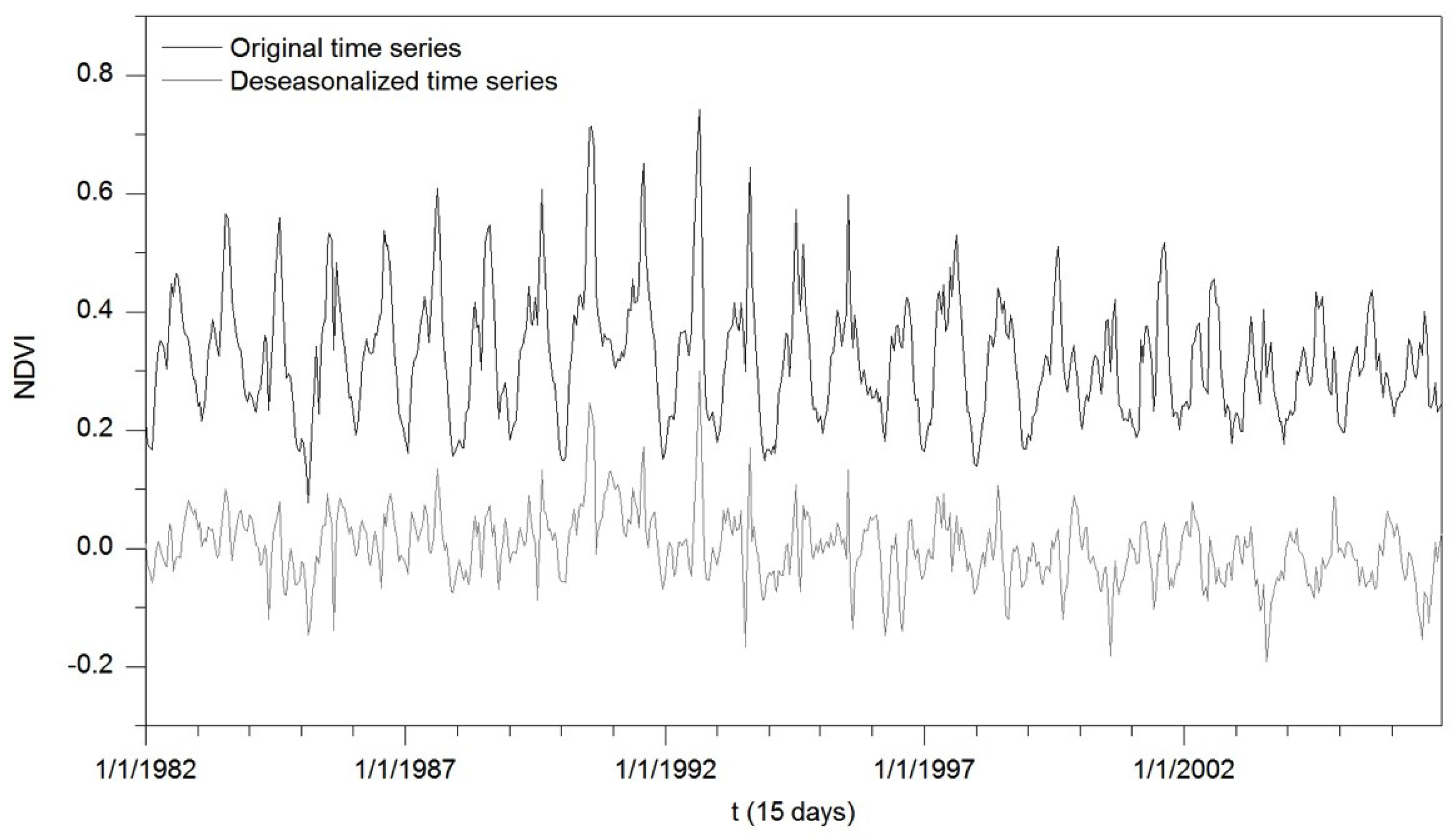
2.1. GIMMS NDVI Dataset and Pre-Processing

The GIMMS NDVI dataset was used as a proxy for vegetation dynamics in this study. The NDVI dataset was downloaded from the website of the Environmental and Ecological Science Data Center for West China, National Natural Science Foundation of China [41], and was acquired by the NOAA-AVHRR series sensors (NOAA 7, 9, 11, 14, 16, 17, and 18) over a 25-year period from July 1981 to December 2006. The dataset has an 8 × 8 km spatial resolution and is composed of approximately 15-day intervals using the maximum value composite (MVC) method [42]. The GIMMS NDVI has been corrected for sensor calibration, sensor degradation and contamination, view geometry, and volcanic aerosols issues [43]. As the dataset did not cover the entire year of 1981, we selected January 1982 as the beginning time point of the analysis. Therefore, 600 images were utilized in this study. Trends in the GIMMS NDVI dataset compared favorably with trends derived from Landsat [44] and MODIS NDVI [45]; moreover, it covers a longer period than other available NDVI datasets. The dataset has been widely applied to monitor long-term and large-scale trends in vegetation dynamics in various regions of the world [3,6,8,13,20,21].
To detect the exact temporal scaling behavior of the NDVI time series, we focused on the departure of the NDVI from the mean 15-day composition. The seasonal cycle was removed from the original NDVIi time series before applying the method. The process works as follows:
x i = N D V I i N D V I j ¯
where xi is the deseasonalized time series, i ranges from 1 to 600, N D V I j ¯ is the average value for each 15-day composition in all years in the record, and j ranges from 1 to 24. Figure 1 shows an example of the original NDVIi and the deseasonalized time series xi of one arbitrary pixel for the study period. The deseasonalized time series exhibits irregular behavior that is primarily related to the inter-annual changes exhibited by climate variables, such as temperature and precipitation.
Figure 1. Characteristic fluctuation of the original and deseasonalized GIMMS NDVI time series for one arbitrary pixel from 1982 to 2006.
Remotesensing 07 12942 g001
To better understand the DFA method and temporal scaling behavior, we randomly selected 10 pixels distributed across China (Figure 2). The selected pixels were used to test the effectiveness of DFA at the individual pixel scale in China based on the GIMMS NDVI time series.
Additionally, to confirm whether the temporal scaling behavior of the raw time series is indicative of long-range correlations or a broad probability density function [46,47], we processed a shuffled deseasonalized time series using a phase randomized method [48] for all of the selected pixels. All of the shuffled series were randomly rearranged 107 times to ensure that the time series were completely random. These shuffled series were not affected by any probability distribution functions. Moreover, the temporal ordering of the raw time series was broken.

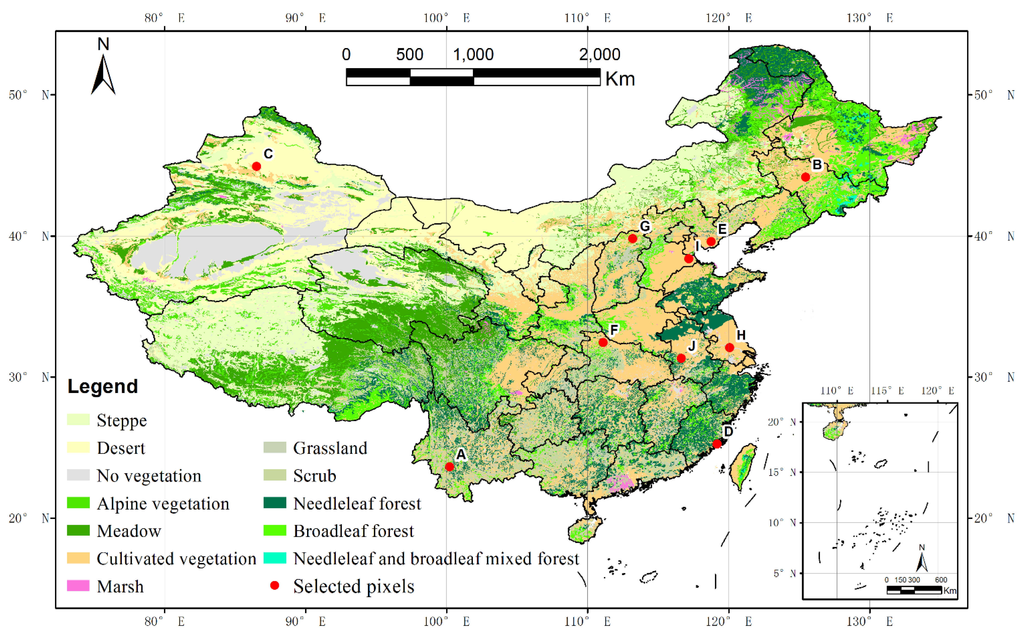
2.2. Vegetation Map of China

The Vegetation Map of China [49], which had a scale of 1:1,000,000, was employed to identify vegetation types in this study. This map was obtained from the Environment and Ecological Science Data Center for West China, National Natural Science Foundation of China [41]. It is shown in Figure 2 and contains numerous polygons that are categorized into 12 types: needleleaf forest, needleleaf and broadleaf mixed forest, broadleaf forest, scrub, grassland, steppe, meadow, marsh, alpine vegetation, desert, cultivated vegetation, and no vegetation. The “no vegetation” type describes regions without any vegetation covering the land surface. This type represents an important biome group in China, and it was regarded as equal to the other vegetation types in the study. The map was used to analyze differences in the temporal scaling behavior of the NDVI time series among various vegetation types.
Figure 2. The vegetation map of China and the locations of selected pixels. The vegetation types of selected pixels are following: A-Scrub, B-Cultivated vegetation, C-Desert, D-Needleleaf forest, E-Cultivated vegetation, F-Alpine vegetation, G-Alpine vegetation, H-Cultivated vegetation, I-Cultivated vegetation, J-Needleleaf forest.
Remotesensing 07 12942 g002

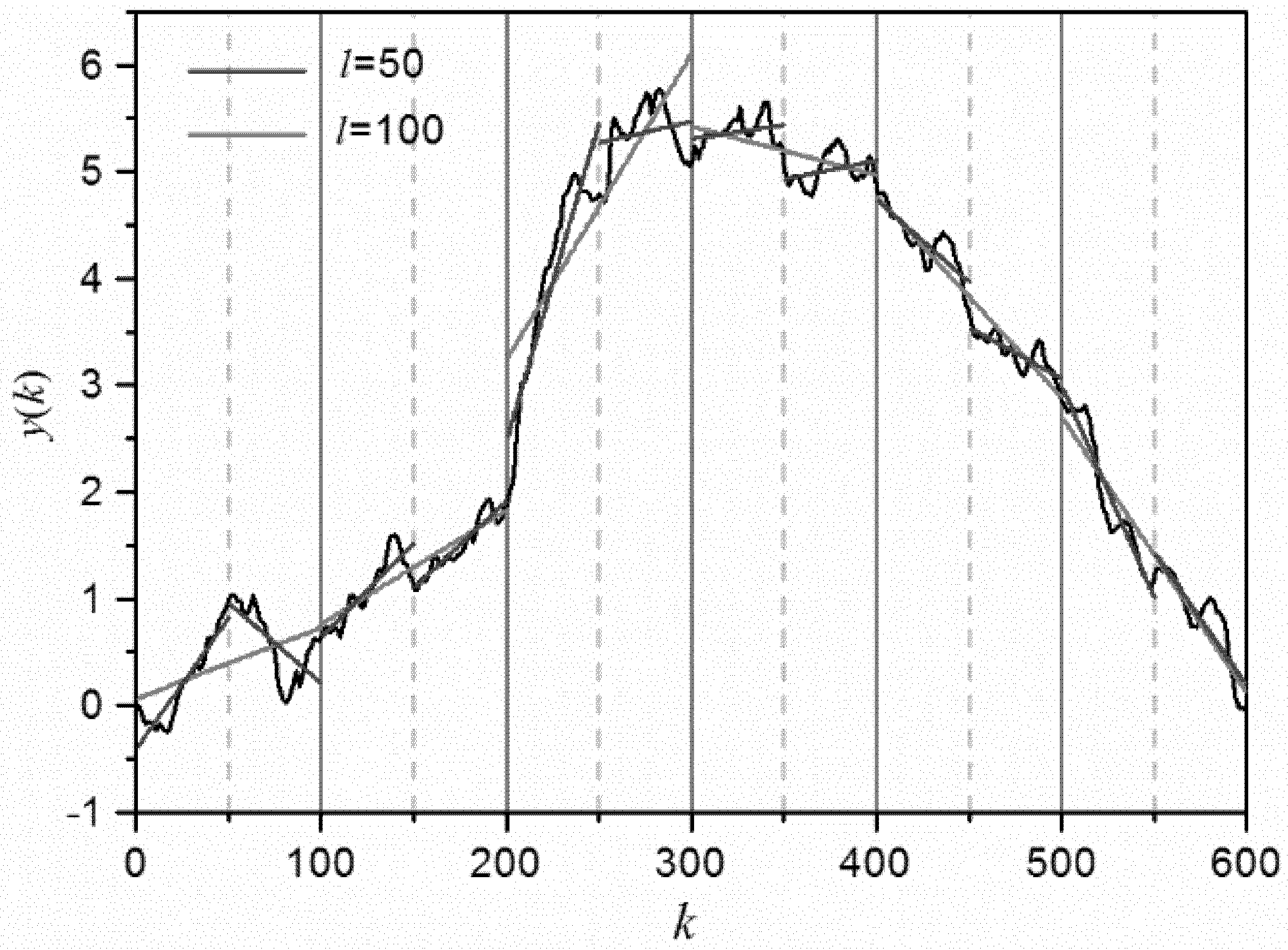
2.3. Detrended Fluctuation Analysis (DFA)

DFA stems from random walk theory and has been effectively used to explore the scaling behavior of natural process time series in diverse fields, such as weather records [25,35], tree-ring width [50], intervention time series of forest fires [31,46], groundwater systems [51], and features of atmosphere [52,53]. DFA provides a simple quantitative parameter to represent the properties of the scaling behavior of complex systems [54].
Consider a deseasonalized time series xi, where i = 1, 2, 3, …, N. N is the length of the series, which is 600 in this study. We first calculate the average of the deseasonalized series xi as follows:
x ¯ = 1 N i = 1 N x i
where x ¯ is the average value of the series xi. We then integrate the series xi:
y ( k ) = i = 1 k ( x i x ¯ )
The bounded series xi is thus converted to an unbounded series y(k), which is the profile of the deseasonalized time series, where k is the order of the time series.
Next, the integrated series y(k) is divided into non-overlapping windows of equal length l, where there are a total of N/l windows for a particular l.
To represent the local trend in each window, the least squares fitting method is used to fit the linear trend yl(k), which is the local trend of each window for a particular length l. The integrated series is detrended by subtracting the local linear trend curve yl(k) in each window. Figure 3 illustrates the local trend of the deseasonalized series for a single pixel in the study area fitted using the linear least squares method with a window length of 50 (blue line) and 100 (red line). In Figure 3, the fluctuation takes a parabola-like shape, which means that the deseasonalized series of anomalies at various times are cumulated. The local trend changes as a function of the window length, suggesting that the local trend of each window depends on the window length.
Figure 3. Application of local linear fitting to the integrated series divided into window lengths of 50 and 100 at a single pixel.
Remotesensing 07 12942 g003
The root-mean-square fluctuation F(l) of this integrated series is calculated after the detrending procedure using the following equation:
F ( l ) = 1 N k = 1 N [ y ( k ) y l ( k ) ] 2
Generally, the window length l ranges from 4 to N/4. Therefore, we repeated the calculations outlined in Equation (4) for different window lengths l, i.e., 4 to 150. We can obtain the variances F(l) as a function of window length l.
We focus on the relationship between F(l) and the window length l for different window length. If the series is characterized by long-range correlation, then F(l)~l has a linear relationship in log-log plots:
log [ F ( l ) ] = α log ( l )
where α is an exponent obtained by measuring the slope of the line that relates log[F(l)] to log(l). The numerical value of α implies that the characteristics of scaling behavior and self-similar process for fluctuations of a series. Different exponents represent different types of scaling behavior in the original series. When α is less than 0.5, the time series exhibits short-range correlation or anti-correlation behavior [25,29,31,46] suggesting that the fluctuation of the series at different times are oppositely correlated and the opposite correlation is the strongest when α closes to 0; when α is around 0.5, the series corresponds to white noise (there is no correlation in the series), i.e., it is a random series; if a long-range correlation exists in the series, α is between 0.5 and 1 [29,31,34,36,46], and the series exhibits power-law behavior meaning that the fluctuation of the series at different times are positively correlated and the positive correlation is the strongest when α closes to 1; when α is equal to 1, the series exhibits characteristics of 1/f noise [31,46], thereby indicating that the series shows a self-organized criticality [55]; and when α is bigger than 1, long-range correlation exists in the series, although it does not obey a power-law relationship [31].

3. Results

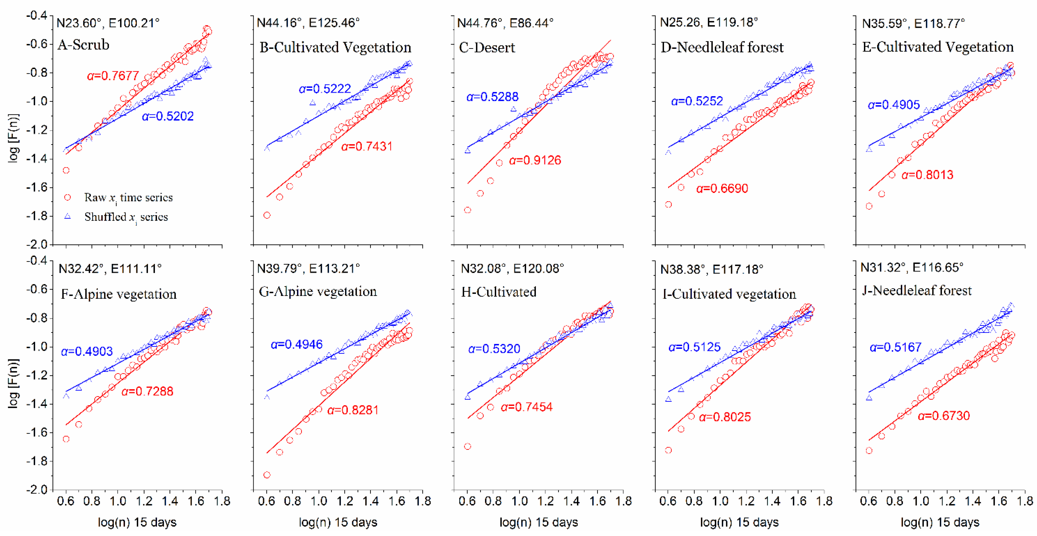
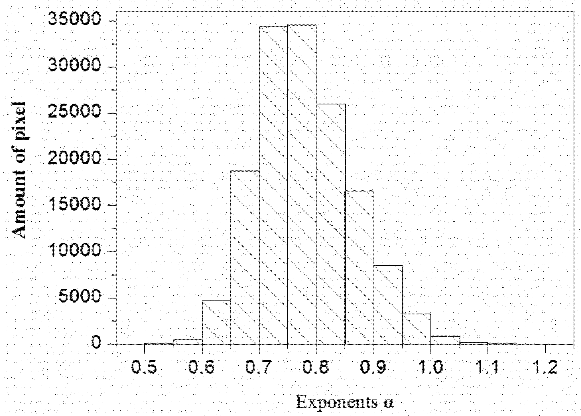
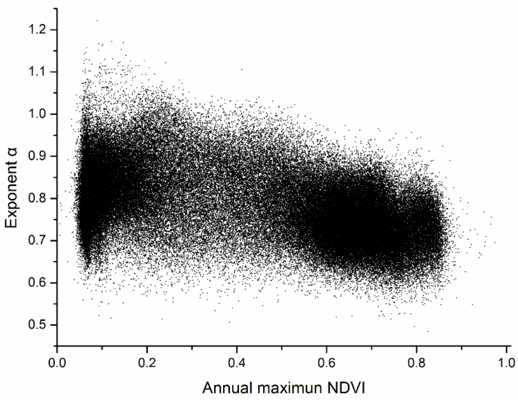
3.1. Temporal Scaling Behavior of the NDVI Time Series at the Pixel Scale

To understand the detailed characteristics of the root-mean-square series, we first performed DFA to determine the temporal scaling behavior of the NDVI time series for all of the selected pixels in China. In Figure 4, a coincident linear feature can be identified in all of the log-log plots. This feature indicates that temporal scaling behaviors exist in the NDVI time series for the selected pixels, suggesting that the NDVI values are correlated at different times. Figure 4 shows that the exponent α ranges from 0.6690 to 0.9126 for all of the log-log plots and that all of the coefficients of determination r exceed 0.99, which is a high value and indicative of statistical significance. The corresponding correlation function suggests long-range correlation exists in the NDVI time series for all of the selected pixels. As a consequence, the temporal scaling behavior can be interpreted as the internal self-similarity of the NDVI time series or as the “memory” within the series at these pixels.
Figure 4. The root-mean-square series and DFA results of fitting for the NDVI time series (red) and shuffled series (blue) at the individual pixel scale.
Remotesensing 07 12942 g004
To confirm whether the temporal scaling behavior of the raw NDVI time series is indicative of long-range correlations or a broad probability density function, DFA was applied to the shuffled NDVI series based on all of the selected pixels. As expected, the exponents of the shuffled series are approximately 0.5 for all of the selected pixels (see Figure 4). According to the computed exponents, all of the shuffled series exhibit approximately random characteristics. Although the raw time series (xi) and the shuffled series have the same population distributions, the different temporal ordering of the two series leads to different scaling behavior. This finding confirms that the temporal scaling behavior of the NDVI time series results from long-range correlation.

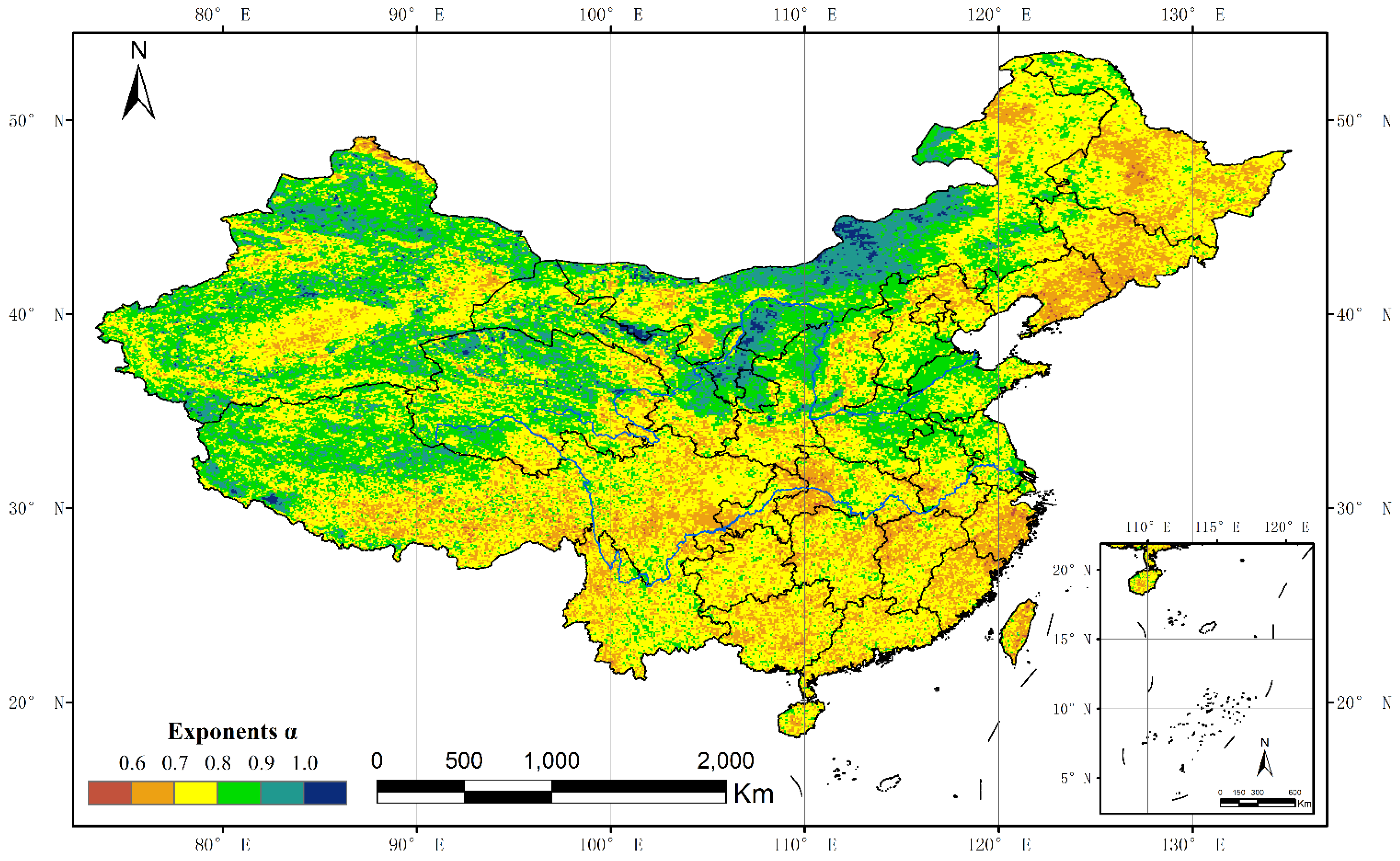
3.2. Spatial Patterns of the Temporal Scaling Behavior of the NDVI Time Series

Because the temporal scaling behavior was found to vary at the pixel scale, we were interested in the regional scale characteristics of the NDVI time series. Therefore, DFA was applied to the entire country of China. Figure 5 shows the results. The exponents of the NDVI time series range from 0.4843 to 1.2215 for all of China. The spatially averaged exponent is 0.7786 with a standard deviation of 0.0819. Figure 5 reveals well-defined variability in the spatial patterns of the exponent during the period studied. These spatial patterns demonstrate that the temporal scaling behavior of the NDVI time series exists over broad scales in China.
As shown in Figure 5, the exponent exhibits complex and fragmented patterns. Values below 0.8 are most frequently observed south of the geographical border of the Qinling Mountains-Huaihe River (0.7283), the southern Qinghai-Tibet Plateau (0.7506), most of northeastern China and the central Tarim Basin (0.7649). In contrast, the remaining regions in China, i.e., most parts of northwestern China, the central Songliao Plain (0.8234) and the North China Plain (0.8135), have exponents exceeding 0.8, which is above the spatial average. The highest exponents, i.e., α > 1, are primarily distributed over the middle of the Hexi Corridor, the Hetao Region, and the central Inner Mongolian Plateau. Based on the above analysis, there is no universal exponent at the regional scale. The temporal scaling behavior of the NDVI time series exhibits well-defined heterogeneity that corresponds to individual geographical regions. For a better understanding of the spatial pattern of temporal scaling behavior, we produced a box-plot of exponents based on latitude (Figure 6). Figure 6 shows that entire pixels of NDVI time series show power-law long-range correlations in the < 25° latitude zone. The range of standard deviation of exponents α is extended from the < 25° to 40°~45° latitude zone. The exponent α values of higher latitude zones display more diverse characteristics, especially within the 40°~45° latitude zone.
We analyzed all of the pixels in China over the range of the exponent α values which are as shown in Figure 7. DFA was performed to process 148,183 pixels in the study. The exponent values were found to range from 0.5 to 1, which is indicative of power-law behavior and is representative of 99.30% of the pixels. Therefore, long-range correlation behavior in the NDVI time series is common throughout China. Additionally, only two pixels have exponent values of below 0.5; these pixels are located in the extreme north of Xinjiang Uygur Autonomous Region and covered by meadow. The two pixels exhibit short-range correlation, whereas several other pixels exhibit 1/f noise or non-power-law long-range correlation (1 to 1.22).
Figure 5. Spatial patterns of the exponent α for the GIMMS NDVI time series calculated via DFA for all of China.
Remotesensing 07 12942 g005
Figure 6. The range of DFA exponent α values at various latitudinal zones. The bottom and top of the box are 1st and 3rd quartile, respectively; the band inside the box is median value (2nd quartile); the square inside the box is mean value; the lower and upper crosses are 1st and 99th percentile, respectively; the lower and upper dashes are 1.5 interquartile range of lower and upper quartiles, respectively; and the bottom and top circles are the minimum and maximum values, respectively.
Remotesensing 07 12942 g006
Figure 7. Histogram of the values of the DFA exponent α for China.
Remotesensing 07 12942 g007

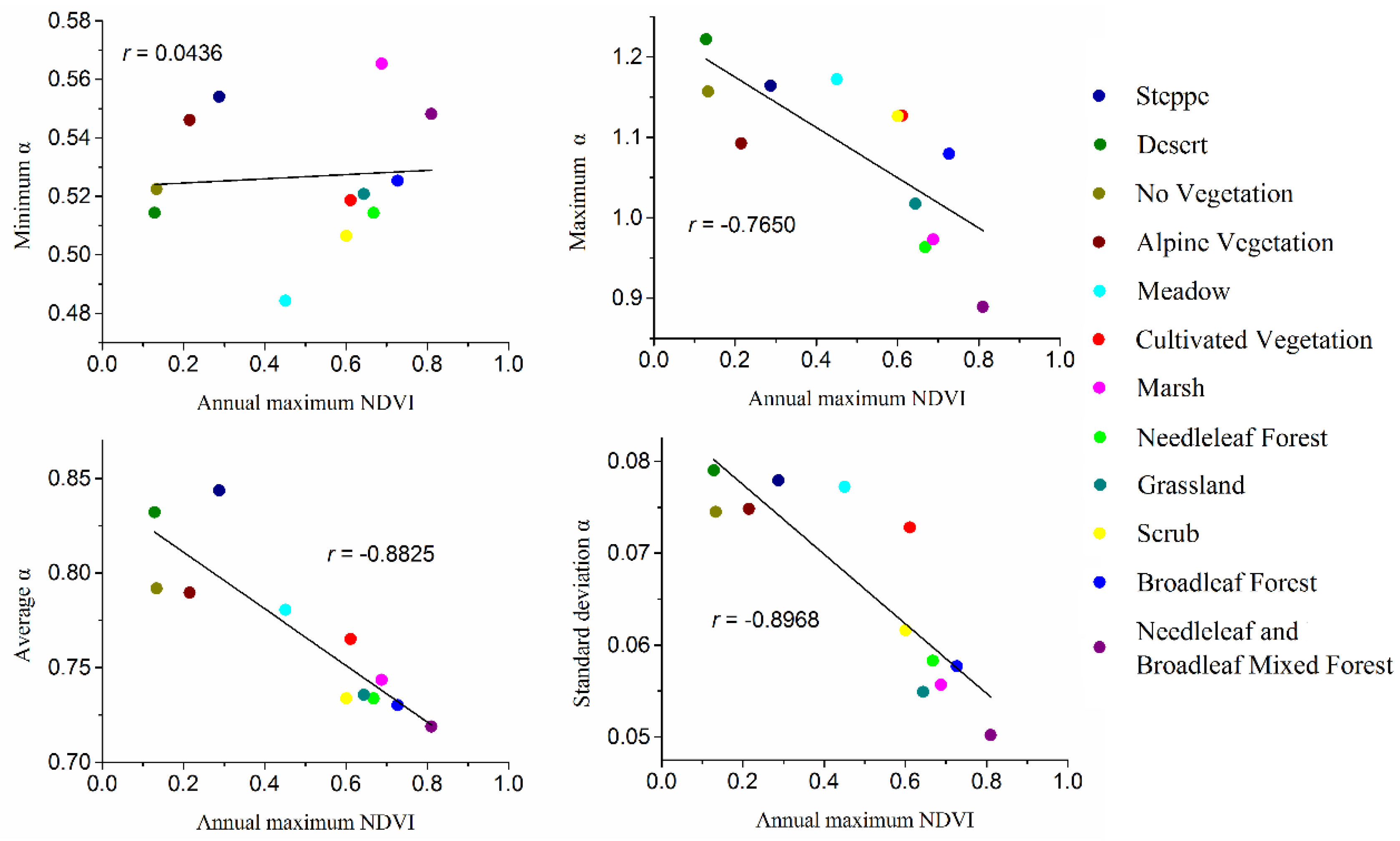
3.3. Characteristics of the Temporal Scaling Behavior for Different Vegetation Types

The NDVI can be used to indicate the activity of vegetation because it exhibits a nearly linear relationship with the fraction of photosynthetically active radiation absorbed by the vegetation canopy and net primary production [56]. We inferred that the temporal scaling behavior of the NDVI time series may be affected by the vegetation type. To confirm this hypothesis, the exponent α values were determined for various vegetation types. The minimum, maximum, and average value, and the standard deviation of exponent α were calculated based on the vegetation map of China. As shown in Table 1, the minimum and maximum exponents are found for meadow and desert, respectively. The average exponent values for all of the vegetation types range from 0.7189 to 0.8436. All of the vegetation types exhibit long-range correlation behavior. The steppe, desert, no vegetation, alpine vegetation, and meadow exponents exceed the spatial average for China (0.7786); the other vegetation types are below the average. Steppe and needleleaf and broadleaf mixed forest exhibit the highest and lowest average exponents for the NDVI time series, respectively.
Table 1. The DFA results of the minimum, maximum, and average exponent α values for all vegetation types.
No.Vegetation Type MinimumMaximumAverage ± SD
1Steppe0.55411.16430.8436 ± 0.0779
2Desert0.51431.22160.8321 ± 0.0790
3No Vegetation0.52241.15690.7918 ± 0.0745
4Alpine Vegetation0.54611.09240.7897 ± 0.0748
5Meadow0.48431.17220.7805 ± 0.0772
6Cultivated Vegetation0.51871.12690.7651 ± 0.0728
7Marsh0.56540.97300.7436 ± 0.0557
8Needleleaf Forest0.51430.96350.7377 ± 0.0583
9Grassland0.52081.01730.7357 ± 0.0549
10Scrub0.50651.12630.7338 ± 0.0616
11Broadleaf Forest0.52531.07950.7302 ± 0.0577
12Needleleaf and Broadleaf Mixed Forest0.54820.88910.7189 ± 0.0502
Figure 8. Scatter plot of exponent α and annual maximum NDVI for all of China.
Remotesensing 07 12942 g008
To further analyze the temporal scaling behaviors for all of China, the annual maximum NDVI was calculated based on the MVC method for the period 1982 to 2006. Figure 8 shows a scatter plot of the exponent α and annual maximum NDVI for all of the pixels in China. As shown in the figure, there is a non-significant trend between annual maximum NDVI and exponent α.
Additionally, the relationships between annual maximum NDVI and the temporal scaling behavior were explored for each vegetation type. The annual maximum NDVI value approximately indicates the green leaf density of the land surface. Figure 9 shows the correlations between the average annual maximum NDVI and the minimum, maximum, and average value, and the standard deviation of the computed exponents for each vegetation type. As indicated in Figure 9, the maximum and average value and standard deviation, but not the minimum value, of the exponent α decrease as the annual maximum NDVI values increase. The correlation coefficients between the maximum and average value, and standard deviation of the exponents and the annual maximum NDVI are −0.7650, −0.8825, and −0.8968, respectively; these correlations are highly significant (p < 0.05).
Figure 9. Relationships between the minimum, maximum, average value and standard deviation of the exponent α and the annual maximum NDVI for each vegetation type.
Remotesensing 07 12942 g009

4. Discussion

In the present study, we applied DFA to investigate the temporal scaling behavior of the NDVI time series. Most pixels, which exhibited exponents from 0.5 to 1, revealed long-range temporal correlation. This finding indicates that the temporal scaling behavior of the NDVI time series exhibits a ubiquitous power-law distribution over most of China. The characteristics do not obey the classical Markov random process (exponential decrease with time), but instead decay slowly as a function of time. Power-law relationships are simple rules that provide the dynamical foundation of the NDVI time series. Meanwhile, the NDVI time series showed a persistent feature that indicates that a positive fluctuation at a particular instant in time is more likely to be followed by a positive fluctuation at the next moment in time. Telesca et al. noted that persistence implied that positive temporal feedback mechanisms drive the dynamics of the NDVI time series [28]. Positive feedback mechanisms tend to destabilize the system under external forces for most of China; these include phenomena such as climate change, fire, and human-caused disturbance. The exponents of two pixels are lower than 0.5, which is regarded as anti-correlation. Thus, the dynamic trends of the NDVI time series in the future will be in direct opposition to those of the present. The 1/f noise, corresponding to exponent values of approximately 1, is considered to be indicative of a self-organizing critical status. This status means that the vegetation is vulnerable; even small changes can produce large variability. Additionally, there are a fraction of pixels of the NDVI time series that show long-range correlation as well as a non-power-law distribution.
From the range of exponents, i.e., 0.5~1, we found that the NDVI time series were consistent with other natural series based on DFA. For example, the exponents of daily mean temperature and relative humidity series are between 0.52 and 0.82 and between 0.60 and 0.95, respectively, for China [25,27], and the exponents for fire sequences range from 0.52 to 0.98 [31]. From the spatial patterns, the temporal scaling behavior of the NDVI time series was found to exhibit common interesting spatial distributions; namely, the exponent α values are higher in most of northern China than in southern China (Figure 5). This feature agrees with the long-range correlation observed in weather and climatology, which are closely related to the dynamics of the NDVI time series. Yuan et al. found that the DFA exponents for temperature decrease with decreasing latitude in China [27]. Moreover, the DFA exponents for relative humidity are higher in northern China than in southern China [25]. Comparing these results and Figure 5, climatology and the NDVI time series have similar geographical patterns. The fundamental mechanisms governing vegetation and climatology may be similar. In addition, a crossover point has been identified for the temperature, fire, and groundwater time series [11,13,22]. We are not clear as to whether such a crossover point exists in the NDVI time series because the bi-weekly NDVI dataset of l, where F(l) can be calculated, is between two months and five years in length in this study. A longer NDVI time series dataset may be required to understand the behavior at longer time scales.
Among the 12 different vegetation types analyzed in this study, strong negative relationships were identified between three types of exponent α values and the annual maximum NDVI (Figure 9). A similar finding has been reported in Mediterranean ecosystems, where the exponents of shrub-land, transitional cover, and forest cover were found to be 1.03, 0.87, and 0.73, respectively [28]. In general, the annual maximum NDVI increases from shrub to forest at the appropriate scales. This characteristic may reflect the fact that these types that showing higher exponent values tend to be more sensitive to external factors [28]. It is well known that climatic variables (e.g., temperature and precipitation) play important roles in NDVI trends [21]. According to the vegetation map of China, the vegetation types with low NDVI, such as steppe, desert, and alpine vegetation, are mainly distributed in northwestern China where there are arid areas. These vegetation types showed significant positive correlations between NDVI and precipitation [57], which suggests that variation in precipitation is the main external factor influencing NDVI dynamics. All of the forest types showed weaker correlations between the NDVI and temperature and precipitation than the other types [57], indicating that forests are not sensitive to climatic variables. However, there was an exception. Typically, the persistence of forest types, i.e., broadleaf forest and needleleaf and broadleaf mixed forest, is weaker than persistence of other types. The average exponent α of needleleaf forest is higher than those of grassland and scrub (see Table 1). Telesca and Lasaponara investigated pre- and post-forest fire temporal scaling behavior based on the SPOT-VGT dataset in Mediterranean ecosystems [29]. Their analysis showed that the post-fire exponent (α = 1.46 ± 0.03) was larger than the pre-fire exponent (α = 1.04 ± 0.06), indicating that fires contribute to increased persistence in temporal vegetation dynamics. Liu et al. reported that needleleaf forest was frequently disturbed by lightning and human-caused fire in the northern Greater Khingan Mountains [58], which was dominated by coniferous species. Therefore, fire is an important factor that causes a relatively strong persistence in needleleaf forest in China. These results indicate that there are different mechanisms driving the various vegetation types. The high exponent values of NDVI time series are caused by more unstable factors.
Few studies have quantified the temporal scaling behavior for vegetation dynamics. Previous studies have been primarily based on spatial power-law relationships. Taylor et al. reported that power-law scaling exponents between the variance of populations and their mean abundances are between 1 and 2, which may explain an underlying fundamental concept in general ecological processes [59]. In another study, it was estimated that the scaling exponents of tree canopies and cluster size distributions range from 0.89 to 2.86 based on IKONOS images for six Kalahari vegetation sites [60]. Here, the calculated exponents based on DFA are between 0.4843 and 1.2215. Because α = (1 + β)/2 [34], where β is the scaling exponent, the temporal scaling exponents of the NDVI time series are between −0.0314 and 1.4430. Compared with previous studies that focused on the spatial scaling behavior, the temporal scaling exponents presented herein are markedly lower than general spatial scaling exponents, suggesting substantial differences in scaling behavior between temporal and spatial ecological processes.
For 1982~2003, the results of Hurst (H) exponent-based R/S analysis were consistent with the GIMMS NDVI dynamics trends in most of the Qinghai-Tibet Plateau basin [3]. However, the spatial pattern of the H exponent was inconsistent with α in the present study for the same area. R/S and DFA analyses have been used as estimators of long-range correlations. Weron noted that DFA analysis outperforms R/S analysis for Gaussian white noise [61] because DFA analysis avoids the spurious correlation of non-stationary series. Moreover, differences in the time period of the NDVI dataset under study could affect the results.

5. Conclusions

DFA was performed to quantify the temporal scaling behavior of the bi-weekly GIMMS NDVI time series for a 25-year period at individual pixel and regional scales. We also discussed variation among vegetation types based on the vegetation map of China. DFA provided a good understanding of the temporal scaling behavior of the NDVI time series in China. We found that the NDVI time series showed a long-range correlation in most of China as suggested by the values of the exponents, which were between 0.5 and 1. However, the DFA exponent was not universal and depended on the geographic location. All of the vegetation types exhibited similar persistent power-law correlations with exponents ranging from 0.7189 to 0.8436. Steppe and broadleaf mixed forest had the strongest and weakest persistence, respectively. Furthermore, there was a general tendency for persistence to increase with decreasing annual maximum NDVI values for different vegetation types, although there were a few exceptions.
The power-law behavior in the temporal evolution of the NDVI time series might reflect short- and long-term vegetation characteristics. Our results suggest that there is a positive temporal feedback in the NDVI time series in China. A positive circularity leads to a growth-generating phenomenon. Furthermore, the vegetation in China departs equilibrium and continuously evolves to self-organizing critical status under this positive temporal feedback.
The results of this study should be relevant to future vegetation and climatic models. However, a more comprehensive understanding of the temporal scaling behavior must be attained in future studies. This study was limited by the availability of NDVI time series data. Finer temporal resolutions and longer temporal spans may lead to a deeper understanding of the processes underlying the temporal scaling behavior of vegetation in the future.

Acknowledgments

This work was supported by the “State Key Laboratory of Resources and Environmental Information System,” the “Fundamental Research Funds for the Central Universities” (Project No. 14QIVJJ025 and 11SSXT134), and the National Natural Science Foundation of China (No. 41201082). We would like to thank Hongshi He, Eckart Dege, Kay Dege, the China Scholarship Council, and the anonymous reviewers.

Author Contributions

Xiaoyi Guo and Hongyan Zhang conceived and designed the experiments. Xiaoyi Guo and Jianjun Zhao performed the experiments. Hongyan Zhang, Tao Yuan, and Zhenshan Xue analyzed the data. Xiaoyi Guo, Tao Yuan, and Jianjun Zhao contributed the materials and analysis tools. Xiaoyi Guo and Hongyan Zhang wrote the paper.

Conflicts of Interest

The authors declare no conflict of interest.

References

  1. Godínez-Alvarez, H.; Herrick, J.E.; Mattocks, M.; Toledo, D.; van Zee, J. Comparison of three vegetation monitoring methods: Their relative utility for ecological assessment and monitoring. Ecol. Indic. 2009, 9, 1001–1008. [Google Scholar] [CrossRef]
  2. Du, J.; Shu, J.; Yin, J.; Yuan, X.; Jiaerheng, A.; Xiong, S.; He, P.; Liu, W. Analysis on spatio-temporal trends and drivers in vegetation growth during recent decades in Xinjiang, China. Int. J. Appl. Earth Obs. Geoinf. 2015, 38, 216–228. [Google Scholar] [CrossRef]
  3. Peng, J.; Liu, Z.; Liu, Y.; Wu, J.; Han, Y. Trend analysis of vegetation dynamics in Qinghai–Tibet Plateau using Hurst Exponent. Ecol. Indic. 2012, 14, 28–39. [Google Scholar] [CrossRef]
  4. Herrmann, S.M.; Anyamba, A.; Tucker, C.J. Recent trends in vegetation dynamics in the African Sahel and their relationship to climate. Glob. Environ. Change 2005, 15, 394–404. [Google Scholar] [CrossRef]
  5. Dubovyk, O.; Landmann, T.; Erasmus, B.F.N.; Tewes, A.; Schellberg, J. Monitoring vegetation dynamics with medium resolution MODIS-EVI time series at sub-regional scale in southern Africa. Int. J. Appl. Earth Obs. Geoinf. 2015, 38, 175–183. [Google Scholar] [CrossRef]
  6. De Jong, R.; de Bruin, S.; de Wit, A.; Schaepman, M.E.; Dent, D.L. Analysis of monotonic greening and browning trends from global NDVI time-series. Remote Sens. Environ. 2011, 115, 692–702. [Google Scholar] [CrossRef] [Green Version]
  7. Barichivich, J.; Briffa, K.R.; Myneni, R.B.; Osborn, T.J.; Melvin, T.M.; Ciais, P.; Piao, S.; Tucker, C. Large-scale variations in the vegetation growing season and annual cycle of atmospheric CO2 at high northern latitudes from 1950 to 2011. Glob. Change Biol. 2013, 19, 3167–3183. [Google Scholar] [CrossRef] [PubMed]
  8. Suzuki, R.; Masuda, K.; Dye, D.G. Interannual covariability between actual evapotranspiration and PAL and GIMMS NDVIs of Northern Asia. Remote Sens. Environ. 2007, 106, 387–398. [Google Scholar] [CrossRef]
  9. Fu, B.; Li, S.; Yu, X.; Yang, P.; Yu, G.; Feng, R.; Zhuang, X. Chinese ecosystem research network: Progress and perspectives. Ecol. Complex. 2010, 7, 225–233. [Google Scholar] [CrossRef]
  10. Lanorte, A.; Lasaponara, R.; Lovallo, M.; Telesca, L. Fisher–Shannon information plane analysis of SPOT/VEGETATION Normalized Difference Vegetation Index (NDVI) time series to characterize vegetation recovery after fire disturbance. Int. J. Appl. Earth Obs. Geoinf. 2014, 26, 441–446. [Google Scholar] [CrossRef]
  11. Tucker, C.J. Red and photographic infrared linear combinations for monitoring vegetation. Remote Sens. Environ. 1979, 8, 127–150. [Google Scholar] [CrossRef]
  12. Xu, G.; Zhang, H.; Chen, B.; Zhang, H.; Innes, J.; Wang, G.; Yan, J.; Zheng, Y.; Zhu, Z.; Myneni, R. Changes in vegetation growth dynamics and relations with climate over China’s landmass from 1982 to 2011. Remote Sens. 2014, 6, 3263–3283. [Google Scholar] [CrossRef]
  13. Zhao, J.; Wang, Y.; Hashimoto, H.; Melton, F.S.; Hiatt, S.H.; Zhang, H.; Nemani, R.R. The variation of land surface phenology from 1982 to 2006 along the Appalachian trail. IEEE Trans. Geosci. Remote Sens. 2013, 51, 2087–2095. [Google Scholar] [CrossRef]
  14. Hou, G.; Zhang, H.; Wang, Y. Vegetation dynamics and its relationship with climatic factors in the Changbai Mountain Natural Reserve. J. Mt. Sci. 2011, 8, 865–875. [Google Scholar] [CrossRef]
  15. Lu, L.; Kuenzer, C.; Wang, C.; Guo, H.; Li, Q. Evaluation of three MODIS-derived vegetation index time series for dryland vegetation dynamics monitoring. Remote Sens. 2015, 7, 7597–7614. [Google Scholar] [CrossRef]
  16. Jeong, S.J.; Ho, C.H.; Choi, S.D.; Kim, J.; Lee, E.J.; Gim, H.J. Satellite data-based phenological evaluation of the nationwide reforestation of South Korea. PLoS ONE 2013, 8, e58900. [Google Scholar] [CrossRef] [PubMed] [Green Version]
  17. Fensholt, R.; Langanke, T.; Rasmussen, K.; Reenberg, A.; Prince, S.D.; Tucker, C.; Scholes, R.J.; Le, Q.B.; Bondeau, A.; Eastman, R.; et al. Greenness in semi-arid areas across the globe 1981–2007—An earth observing satellite based analysis of trends and drivers. Remote Sens. Environ. 2012, 121, 144–158. [Google Scholar] [CrossRef]
  18. Martínez, B.; Gilabert, M.A. Vegetation dynamics from NDVI time series analysis using the wavelet transform. Remote Sens. Environ. 2009, 113, 1823–1842. [Google Scholar] [CrossRef]
  19. Schucknecht, A. Assessing vegetation variability and trends in north-eastern Brazil using AVHRR and MODIS NDVI time series. Eur. J. Remote Sens. 2013, 40–59. [Google Scholar] [CrossRef]
  20. Sobrino, J.A.; Julien, Y. Global trends in NDVI-derived parameters obtained from GIMMS data. Int. J. Remote Sens. 2011, 32, 4267–4279. [Google Scholar] [CrossRef]
  21. Piao, S.; Fang, J.; Zhou, L.; Guo, Q.; Henderson, M.; Ji, W.; Li, Y.; Tao, S. Interannual variations of monthly and seasonal normalized difference vegetation index (NDVI) in China from 1982 to 1999. J. Geophys. Res. 2003, 108, 1–12. [Google Scholar] [CrossRef]
  22. Chuai, X.W.; Huang, X.J.; Wang, W.J.; Bao, G. NDVI, temperature and precipitation changes and their relationships with different vegetation types during 1998–2007 in Inner Mongolia, China. Int. J. Climatol. 2013, 33, 1696–1706. [Google Scholar] [CrossRef]
  23. Sun, Y.; Yan, X.; Xie, D. Study on the relationship between vegetation and climate in China using factor analysis. J. Mt. Sci. 2007, 25, 54–63. [Google Scholar]
  24. Wu, D.H.; Zhao, X.; Zhao, W.Q.; Tang, B.J.; Xu, W.F. Response of vegetation to temperature, precipitation and solar radiation time-scales: A case study over mainland Australia. In Proceedings of 2014 IEEE International Geoscience and Remote Sensing Symposium (IGARSS), QC, Canada, 13–18 July 2014.
  25. Lin, G.; Chen, X.; Fu, Z. Temporal-spatial diversities of long-range correlation for relative humidity over China. Phys. Stat. Mech. Appl. 2007, 383, 585–594. [Google Scholar] [CrossRef]
  26. Osokin, A.R.; Podlazov, A.V.; Chernetsky, V.A.; Livshits, M.A. Solar flares: Self-organization of active region to the critical state. Proc. Int. Astron. Union 2004, 2004, 477–478. [Google Scholar] [CrossRef]
  27. Yuan, N.; Fu, Z.; Mao, J. Different scaling behaviors in daily temperature records over China. Phys. Stat. Mech. Appl. 2010, 389, 4087–4095. [Google Scholar] [CrossRef]
  28. Telesca, L.; Lasaponara, R.; Lanorte, A. Intra-annual dynamical persistent mechanisms in mediterranean ecosystems revealed SPOT-VEGETATION time series. Ecol. Complex. 2008, 5, 151–156. [Google Scholar] [CrossRef]
  29. Telesca, L.; Lasaponara, R. Pre- and post-fire behavioral trends revealed in satellite NDVI time series. Geophys. Res. Lett. 2006. [Google Scholar] [CrossRef]
  30. Poveda, G.; Salazar, L.F. Annual and interannual (ENSO) variability of spatial scaling properties of a vegetation index (NDVI) in Amazonia. Remote Sens. Environ. 2004, 93, 391–401. [Google Scholar] [CrossRef]
  31. Zheng, H.; Song, W.; Satoh, K. Detecting long-range correlations in fire sequences with detrended fluctuation analysis. Phys. Stat. Mech. Appl. 2010, 389, 837–842. [Google Scholar] [CrossRef]
  32. Alvarez-Ramirez, J.; Rodriguez, E.; Echeverria, J.C. A DFA approach for assessing asymmetric correlations. Phys. Stat. Mech. Appl. 2009, 388, 2263–2270. [Google Scholar] [CrossRef]
  33. Pinzon, J.; Tucker, C. A non-stationary 1981–2012 AVHRR NDVI3g time series. Remote Sens. 2014, 6, 6929–6960. [Google Scholar] [CrossRef]
  34. Peng, C.K.; Buldyrev, S.V.; Havlin, S.; Simons, M.; Stanley, H.E.; Goldberger, A.L. Mosaic organization of DNA nucleotides. Phys. Rev. 1994, 49, 1685–1689. [Google Scholar] [CrossRef]
  35. Király, A.; Jánosi, I.M. Detrended fluctuation analysis of daily temperature records: Geographic dependence over Australia. Meteorol. Atmos. Phys. 2004, 88, 119–128. [Google Scholar] [CrossRef]
  36. Zhao, Z.D.; Cai, S.M.; Huang, J.; Fu, Y.; Zhou, T. Scaling behavior of online human activity. Europhys. Lett. 2012, 100, 48004–48009. [Google Scholar] [CrossRef]
  37. Fang, J.; Piao, S.; Field, C.B.; Pan, Y.; Guo, Q.; Zhou, L.; Peng, C.; Tao, S. Increasing net primary production in China from 1982 to 1999. Front. Ecol. Environ. 2003, 1, 293–297. [Google Scholar] [CrossRef]
  38. Fang, J.; Piao, S.; Tang, Z.; Peng, C.; Ji, W. Interannual variability in net primary production and precipitation. Science 2001, 293, 1723–1723. [Google Scholar] [CrossRef] [PubMed]
  39. Zhao, Y.; He, C.; Zhang, Q. Monitoring vegetation dynamics by coupling linear trend analysis with change vector analysis: A case study in the Xilingol steppe in northern China. Int. J. Remote Sens. 2012, 33, 287–308. [Google Scholar] [CrossRef]
  40. Yang, J.; Ding, Y.; Chen, R. Spatial and temporal of variations of alpine vegetation cover in the source regions of the Yangtze and Yellow Rivers of the Tibetan Plateau from 1982 to 2001. Environ. Geol. 2006, 50, 313–322. [Google Scholar] [CrossRef]
  41. Environmental and Ecological Science Data Center for West China, National Natural Science Foundation of China. Available online: http://westdc.westgis.ac.cn/ (accessed on 17 April 2013).
  42. Holben, B.N. Characteristics of maximum-value composite images from temporal AVHRR data. Int. J. Remote Sens. 1986, 7, 1417–1434. [Google Scholar] [CrossRef]
  43. Tucker, C.; Pinzon, J.; Brown, M.; Slayback, D.; Pak, E.; Mahoney, R.; Vermote, E.; Saleous, N. El An extended AVHRR 8-km NDVI dataset compatible with MODIS and SPOT vegetation NDVI data. Int. J. Remote Sens. 2005, 26, 4485–4498. [Google Scholar] [CrossRef]
  44. Beck, H.E.; McVicar, T.R.; van Dijk, A.I.J.M.; Schellekens, J.; de Jeu, R.A.M.; Bruijnzeel, L.A. Global evaluation of four AVHRR–NDVI data sets: Intercomparison and assessment against Landsat imagery. Remote Sens. Environ. 2011, 115, 2547–2563. [Google Scholar] [CrossRef]
  45. Fensholt, R.; Proud, S.R. Evaluation of earth observation based global long term vegetation trends—Comparing GIMMS and MODIS global NDVI time series. Remote Sens. Environ. 2012, 119, 131–147. [Google Scholar] [CrossRef]
  46. Da Silva, L.R.; Stošić, T.; Stošić, B.D. Power law correlations in time series of wild-land and forest fires in Brazil. Int. J. Remote Sens. 2012, 33, 2059–2067. [Google Scholar] [CrossRef]
  47. Kantelhardt, J.W.; Koscielny-Bunde, E.; Rego, H.H.; Havlin, S.; Bunde, A. Detecting long-range correlations with detrended fluctuation analysis. Phys. Stat. Mech. Appl. 2001, 295, 441–454. [Google Scholar] [CrossRef]
  48. Theiler, J.; Eubank, S.; Longtin, A.; Galdrikian, B.; Doyne Farmer, J. Testing for nonlinearity in time series: The method of surrogate data. Phys. Nonlinear Phenom. 1992, 58, 77–94. [Google Scholar] [CrossRef]
  49. Editorial Board of Vegetation Map of China. Vegetation Map of the People’s Republic of China (1:1,000,000) 2001. Available online: http://westdc.westgis.ac.cn/ (accessed on 30 May 2013).
  50. Telesca, L.; Lovallo, M. Long-range dependence in tree-ring width time series of Austrocedrus Chilensis revealed by means of the detrended fluctuation analysis. Phys. Stat. Mech. Appl. 2010, 389, 4096–4104. [Google Scholar] [CrossRef]
  51. Li, Z.; Zhang, Y.K. Quantifying fractal dynamics of groundwater systems with detrended fluctuation analysis. J. Hydrol. 2007, 336, 139–146. [Google Scholar] [CrossRef]
  52. Varotsos, C.A.; Ondov, J.M.; Cracknell, A.P.; Efstathiou, M.N.; Assimakopoulos, M.N. Long-range persistence in global Aerosol Index dynamics. Int. J. Remote Sens. 2006, 27, 3593–3603. [Google Scholar] [CrossRef]
  53. Varotsos, C. Power-law correlations in column ozone over Antarctica. Int. J. Remote Sens. 2005, 26, 3333–3342. [Google Scholar] [CrossRef]
  54. Hu, K.; Ivanov, P.; Chen, Z.; Carpena, P.; Eugene Stanley, H. Effect of trends on detrended fluctuation analysis. Phys. Rev. E 2001, 64, 1–19. [Google Scholar] [CrossRef]
  55. Bak, P.; Tang, C.; Wiesenfeld, K. Self-organized criticality. Phys. Rev. A 1988, 38, 364–374. [Google Scholar] [CrossRef]
  56. Gamon, J.A.; Field, C.B.; Goulden, M.L.; Griffin, K.L.; Hartley, A.E.; Joel, G.; Peñuelas, J.; Valentini, R. Relationships between NDVI, canopy structure, and photosynthesis in three Californian vegetation types. Ecol. Appl. 1995, 5, 28–41. [Google Scholar] [CrossRef]
  57. Piao, S.; Fang, J.; Wei, J.; Guo, Q.; Ke, J.; Tao, S. Variation in a satellite-based vegetation index in relation to climate in China. J. Veg. Sci. 2004, 15, 219–226. [Google Scholar] [CrossRef]
  58. Liu, Z.; Yang, J.; Chang, Y.; Weisberg, P.J.; He, H.S. Spatial patterns and drivers of fire occurrence and its future trend under climate change in a boreal forest of Northeast China. Glob. Change Biol. 2012, 18, 2041–2056. [Google Scholar] [CrossRef]
  59. Taylor, L.R.; Perry, J.N.; Woiwod, I.P.; Taylor, R.A.J. Specificity of the spatial power-law exponent in ecology and agriculture. Nature 1988, 332, 721–722. [Google Scholar] [CrossRef]
  60. Scanlon, T.M.; Caylor, K.K.; Levin, S.A.; Rodriguez-Iturbe, I. Positive feedbacks promote power-law clustering of Kalahari vegetation. Nature 2007, 449, 209–212. [Google Scholar] [CrossRef] [PubMed]
  61. Weron, R. Estimating long-range dependence: Finite sample properties and confidence intervals. Phys. Stat. Mech. Appl. 2002, 312, 285–299. [Google Scholar] [CrossRef]

