Article

An Upscaling Algorithm to Obtain the Representative Ground Truth of LAI Time Series in Heterogeneous Land Surface

1
State Key Laboratory of Remote Sensing Science, Research Center for Remote Sensing and GIS, and School of Geography, Beijing Normal University, Beijing 100875, China
2
Beijing Key Laboratory for Remote Sensing of Environment and Digital Cities, Beijing Normal University, Beijing 100875, China
3
Laboratory of Tibetan Environment Changes and Land Surface Processes, Institute of Tibetan Plateau Research, Chinese Academy of Sciences, Beijing 100101, China
*
Author to whom correspondence should be addressed.
Remote Sens. 2015, 7(10), 12887-12908; https://doi.org/10.3390/rs71012887
Submission received: 8 July 2015 / Revised: 26 August 2015 / Accepted: 21 September 2015 / Published: 30 September 2015

Abstract

:
Upscaling in situ leaf area index (LAI) measurements to the footprint scale is important for the validation of medium resolution remote sensing products. However, surface heterogeneity and temporal variation of vegetation make this difficult. In this study, a two-step upscaling algorithm was developed to obtain the representative ground truth of LAI time series in heterogeneous surfaces based on in situ LAI data measured by the wireless sensor network (WSN) observation system. Since heterogeneity within a site usually arises from the mixture of vegetation and non-vegetation surfaces, the spatial heterogeneity of vegetation and land cover types were separately considered. Representative LAI time series of vegetation surfaces were obtained by upscaling in situ measurements using an optimal weighted combination method, incorporating the expectation maximum (EM) algorithm to derive the weights. The ground truth of LAI over the whole site could then be determined using area weighted combination of representative LAIs of different land cover types. The algorithm was evaluated using a dataset collected in Heihe Watershed Allied Telemetry Experimental Research (HiWater) experiment. The proposed algorithm can effectively obtain the representative ground truth of LAI time series in heterogeneous cropland areas. Using the normal method of an average LAI measurement to represent the heterogeneous surface produced a root mean square error (RMSE) of 0.69, whereas the proposed algorithm provided RMSE = 0.032 using 23 sampling points. The proposed ground truth derived method was implemented to validate four major LAI products.

Graphical Abstract

1. Introduction

The leaf area index (LAI), defined as half the total developed area of green leaves per unit ground horizontal surface area [1], is an essential vegetation parameter and plays an important role in crop growth monitoring, yield estimation, ecosystem productivity, and land surface modeling [2,3,4,5,6,7,8]. Remote sensing methods provide an effective way to acquire LAI with different spatial and temporal resolutions [9]. Several medium resolution remote sensing LAI products (250 m–1 km) have been produced, such as MODIS (Medium Resolution Imaging Spectrometer) [10], GEOV1 [11], and GLASS [12], and extensively applied in monitoring seasonal and interannual variation of LAI over regional to global domains. However, the LAI products must be validated against in situ measurements to provide the uncertainties associated with these products, which are essential for their application and improvement of the LAI inversion algorithm [13,14].
Validation of LAI products is a very difficult task, particularly regarding their kilometric spatial resolution and vegetation dynamic changes [14]. The remote sensing footprint is much larger than the representative area of in situ LAI measurement due to surface heterogeneity; therefore, a pragmatic approach is required to upscale in situ measurements to the scale of the satellite footprint. There are two major upscaling schemes for validation of LAI products. The simplest is to average a number of in situ LAI measurements to present the ground truth. This method is promising when a sufficient number of sampling points are available and the site is homogeneous over a large area [15]. However, surface heterogeneity is generally present in medium resolution footprints, and an alternative approach is the bridging method based on the use of high resolution remote sensing images [14,16]. The high resolution map of LAI is first estimated generally based on an empirical transfer function between the radiometric signal and a number of LAI data measured in the whole site. This map is then applied to obtain the ground truth by aggregation of the LAI estimates. Although the bridging method has been recognized as an effective way to obtain the ground truth in the guidelines of the Land Product Validation (LPV) subgroup of the Committee Earth Observing Satellite (CEOS) [14] and widely used in validation studies [17,18,19,20,21,22,23,24,25], its feasibility is influenced by the limited number of high resolution images due to low temporal resolution and cloud aerosol contamination. In addition, the accuracy of the LAI map is impacted by the representativeness of the sampling points for the whole site [16].
Another issue is the in situ LAI measurements. LAI can be measured by direct or indirect methods, but the direct methods are time consuming and cannot be applied routinely [26]. Hence, remote sensing LAI validation experiments rely largely on indirect measurements using optical instruments rather than direct measurements [14]. However, the indirect method is still labor intensive and difficult for obtaining a large number of LAI data over such a large space and a short time period constrained by the satellite revisit time. Therefore, very few validation studies show repeated measurements along the year or between years. There are usually one or two high resolution maps of LAI for a given year and site close to the maximum vegetation development [16,17,18,19,20,21,22,23]. The temporal mismatch between ground based measurement and LAI products can produce uncertainty in validation due to dynamic change of vegetation, especially crops [27,28,29].
The CEOS LPV defines a hierarchical four stage validation approach for the requirement of user communities [30]. LAI products reach stage 2 validation and a dataset of 113 reference values has been acquired through significant international LAI validation activity over several years [30]. However, this is still limited in space and especially in time, which restricts the opportunity to reach a higher validation stage [31]. Some researchers have sought to use the operational algorithms of medium resolution LAI products or advanced sensors with both frequent revisit capacity and decametric spatial resolution to solve this problem [32,33,34,35]. However, ultimately all LAI estimates must be evaluated against in situ LAI measurements.
The ground based measurement method based on wireless sensor networks (WSN) technology is a suitable method for validation and provides a good opportunity to evaluate the temporal consistency of remote sensing products [36,37,38]. The WSN technology allows spatially distributed ground instruments, and can perform automatic temporal monitoring, greatly reducing labor and time costs. In addition, this measurement method is lower cost than commonly used optical instruments, which is critical for ground validation experiments. Qu et al. [39,40] designed the LAINet observation system for LAI measurements based on WSN technology and commenced upscaling these measurements using the bridging method. Qin et al. [41] developed an effective upscaling method for in situ soil moisture measured by the WSN method, which obtained the temporally continuous ground truth of soil moisture. Further studies are required to confirm if this upscaling method is effective for LAI in heterogeneous surfaces.
The objective of this paper was to upscale in situ LAI measurements from the LAINet system to obtain the continuous representative ground truth of LAI in heterogeneous surfaces. The temporal continuous LAI over the period of a crop growth season was called LAI time series, to distinguish it from the separately distributed ground truth over time. Section 2 briefly described the study area and the collected dataset including in situ LAI data, ASTER (Advanced Spaceborne Thermal Emission and Reflection), provided by Heihe Watershed Allied Telemetry Experimental Research (HiWater) experiment. The field experiment was conducted over a 4 km × 4 km area composed of cropland and various non-vegetation types in the Yingke irrigation district in the arid regions of the middle Heihe River, northwest China in 2012. In Section 3, the two-step upscaling algorithm was proposed, considering the heterogeneity of the site from different land cover types. We scaled up in situ measurements with optimal weights to obtain the representative LAI time series of vegetation surface. A cost function was established constrained by ancillary information extracted from ASTER images and the concurrent in situ LAI measurements. The expectation maximum (EM) optimization algorithm was used to determine the weights from this minimization problem. We then scaled up the representative LAI of different land cover types with area weighted method to present the ground truth of LAI over the whole site. In Section 4, the upscaling algorithm was evaluated in the cropland area and the derived ground truth of LAI was used to validate the LAI products. The results were discussed in Section 5, before providing our conclusions in the final section.

2. Study Area and Data

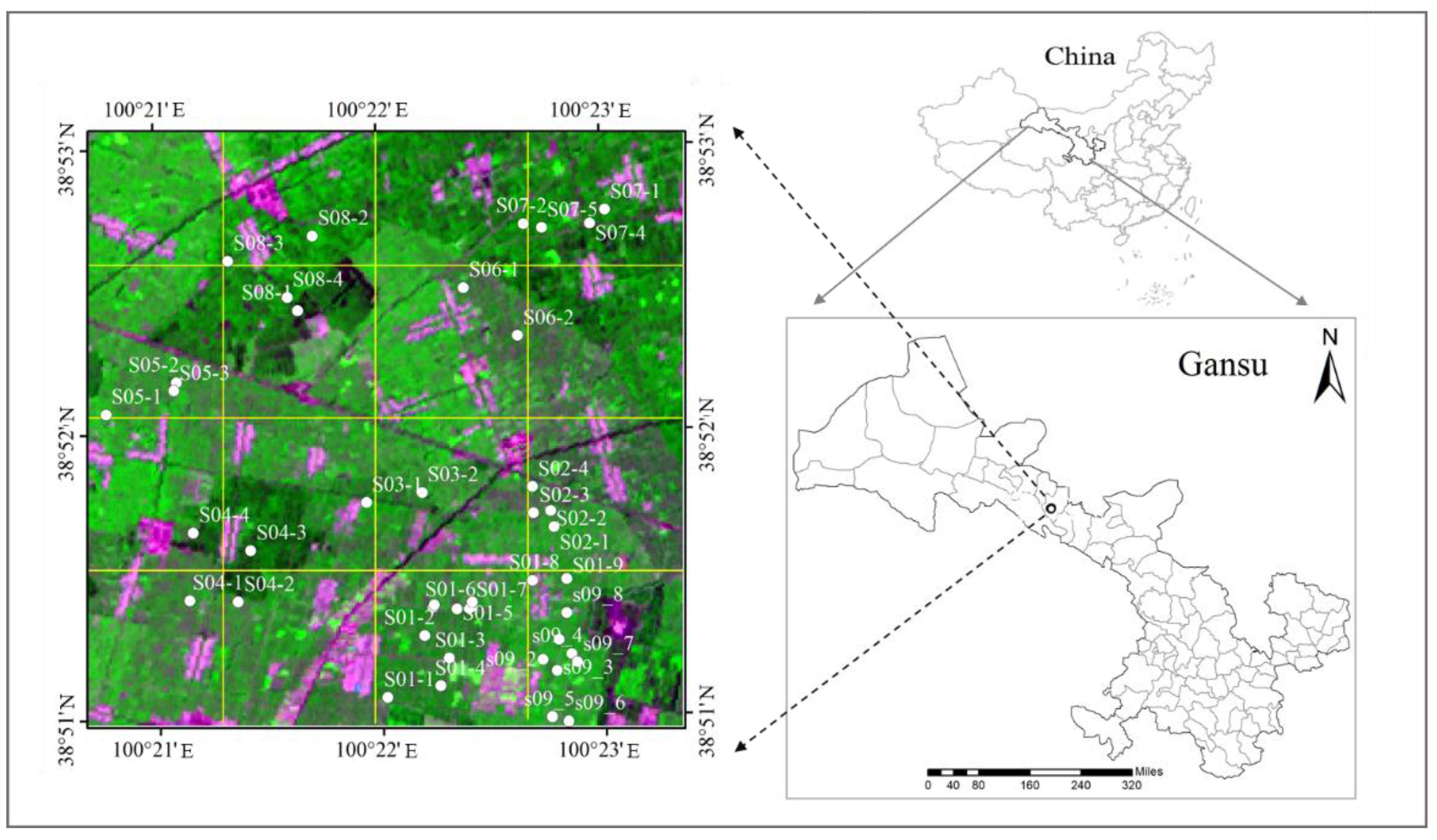
2.1. Study Area and In Situ LAI Data

The field experiment was conducted in the Yingke irrigation district in the arid regions of the middle Heihe River, northwest China (100°22′E, 38°52′N, Figure 1) in 2012. It is a part of the Heihe watershed allied telemetry experimental research (Hi-WATER) project, which is a multi-disciplinary and integrated remote sensing experiment evaluating ecological and hydrological processes in the Heihe River basin [42]. A flat site of 4 km × 4 km was chosen to collect in situ LAI data and meets the general requirement of site size in validation of LAI products [43]. The site was predominantly cultivated with corn (green region in Figure 1), but included numerous residential areas, irrigation facilities, and roads. The spatial differences of corn growth were manifested by the distinct green levels in Figure 1. As a typical row crop, corn was cultivated uniformly with non-continuous gaps, planted in late April and harvested in mid-September of 2012.
Figure 1. Location of the study area (false color composite ASTER image acquired on 24 June 2012, R/G/B vs. band1/band3/band2), 42 sampling points (white points) distributed in 4 km × 4 km area.
Remotesensing 07 12887 g001
In the study area, a LAINet observation system containing 42 WSN measurement nodes was used to measure LAI between 25 June and 24 August 2012. Each measurement node automatically collected multi-angle transmittance of the vegetation canopy during the day and the LAI can be calculated from this based on direct light transmittance algorithm. An approximately uniform sampling method was adopted and each observation node was located in a homogenous zone within the field [40]. Detailed information regarding the LAINet observation system and the field experiment can be found in Qu et al. [39,40].
Every measurement node was employed from June 25 to August 24, governed by vegetation growing season. The corn grew normally, however, not all field measurements were valid due to low battery levels and unexpected weather. To better describe vegetation growth characteristics, an aggregating window of five days was implemented to smooth the LAI data. Moreover, LAI data on August 4 and 14 were excluded from the analysis, due to measurement failures and high temporal variability, respectively. Thus, 42 valid sampling points with 10 measurements at each point were available, as shown in Table 1.
Table 1. The collected ASTER data and four LAI products data including two MODIS C5, GLASS v3.0, and GEOV1 corresponding to the dates of in situ LAI data.
In situ LAIJun.25Jun.30Jul.5Jul.10Jul.15Jul.20Jul.25Jul.30Aug.9Aug.19
ASTERJun.24 Jul.10 Aug.2Aug.11Aug.18
MOD15C5/MCD15C5Jun.25 Jul.3Jul.11 Jul.19Jul.27Aug.4Aug.12Aug.20
GLASS v3.0Jun.25 Jul.3Jul.11 Jul.19Jul.27Aug.4Aug.12Aug.20
GEOV1 Jun.23 Jul.3 Jul.13 Jul.24Aug.3Aug.13Aug.24

2.2. Remote Sensing Data

ASTER imagery was applied to extract ancillary information to support the upscaling investigation. Five high quality ASTER images (2B05V) were acquired corresponding to the dates of field observations (Table 1). ASTER 2B05V data are atmospheric corrected surface reflectance with three bands (0.52–0.86 μm) and 15 m spatial resolution in UTM (WGS84) projection. All images were geometrically corrected to the standard reference image with 0.5 pixel accuracy, which was commonly accepted based on the findings of Gu et al. [44].
Table 2. Characteristics of MODIS, GLASS and GEOV1 LAI products.
LAI ProductsVersionSpatial ResolutionTemporal Resolution (Day)AlgorithmReferences
MOD/MCD15C51.0 km8LUTYang et al. [45]
GLASSV31.0 km8NNXiao et al. [12]
GEOV1V11/112°10NNBaret et al. [11]
Note: LUT and NN refer to the look-up table and neural network methods, respectively.
Several LAI products including two MODIS collection 5 (C5), GLASS v3.0, and GEOV1 (Table 2), were collected and used for comparison with the ground truth of LAI created by the proposed method detailed in Section 3. MODIS C5 products are generated every eight days and have a 1 km spatial resolution (http://wist.echo.nasa.gov) in sinusoidal projection. The main algorithm is based on a lookup table (LUT) simulated from a 3D radiative transfer model, and a backup algorithm based on NDVI is used when the main algorithm fails [45]. The MODIS LAI product suite, containing the Terra C5 (MOD15 C5) and Terra + Aqua C5 (MCD15 C5), were investigated. The 1 km, 8 day, GLASS v3.0 LAI product is available from the Beijing Normal University (BNU) (http://www.bnu-datacenter.com/) in the Integerized Sinusoidal (ISIN) projection. This is estimated from MODIS and AVHRR time series reflectance data using a neural network approach [12]. The European GEOLAND-2 LAI product (GEOV1) is derived from the SPOT/VEGETATION observations at 1/112° (~1 km at the equator) spatial resolution with a 10 day time step in a Plate Carrée projection (http://www.geoland2.eu). It is estimated based on a fusion between MODIS15 and CYCLOPES products [11]. During the field experimental period, eight MODIS and GLASS LAI images, and seven GEOV1 LAI images over the study area were downloaded (Table 1).

3. Methods

3.1. Framework of the Upscaling Algorithm

The land cover of this site was mainly mixed corn and numerous non-vegetation types (i.e., residential areas, irrigation facilities, and roads), while the in situ LAI was only measured in the vegetation area. The in situ LAI measurements continuously acquired at several sampling points could capture the approximate temporal pattern of LAI of the vegetation surface, but might lose fidelity to the true LAI of the vegetation surface in the site level. If a few true LAI of the vegetation surface could be identified, they could be used as ancillary information for upscaling of in situ LAI measurements time series. In this study, information extracted from the high resolution images played such a role. If the representative LAI of vegetation surface was accurately determined, the ground truth of LAI over the whole site could be calculated based on the coverage proportion of vegetation area. A two-step upscaling algorithm is proposed to merge the ancillary information and in situ LAI measurements to obtain ground truth of the LAI time series over the whole site. Figure 2a outlines the flowchart of this method and Figure 2b shows the process of ancillary information.
Figure 2. Flowchart of the two-step upscaling algorithm. (a) The overall procedure, (b) Ancillary information extracted from high resolution images to be used in the upscaling procedure.
Remotesensing 07 12887 g002

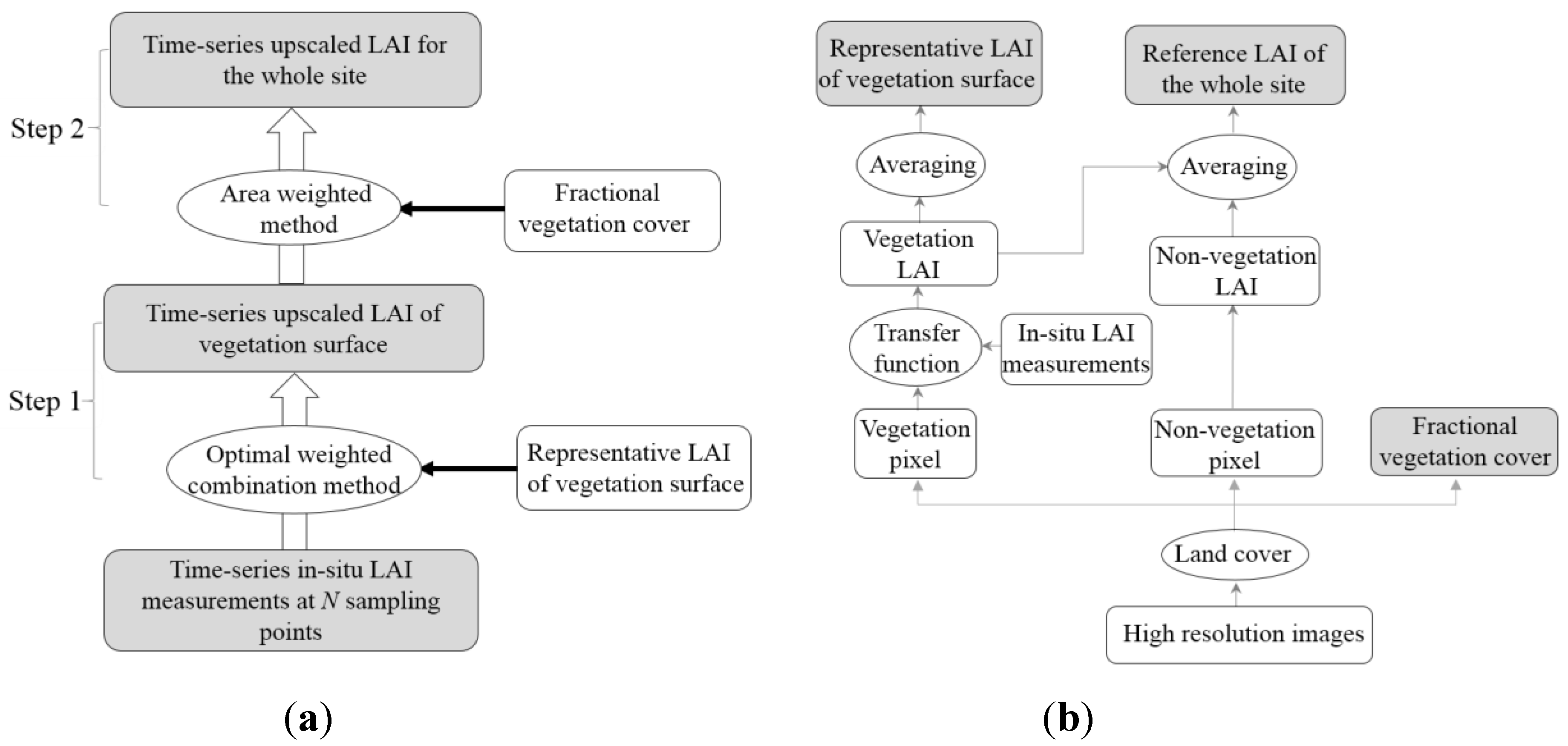
3.1.1. Upscaling In Situ LAI Measurements in the Vegetation Surface

In the first step, for the vegetation surface of this site, the LAI time series were obtained by upscaling the in situ LAI measurements using optimal weighted combination method. The simple averaging method, using equal weight for all measurements, is a popular way to calculate the average LAI from measurements distributed within an area [15]. However, when we consider the spatial difference of vegetation growth over a large area, the weights should be determined by the representativeness of each LAI measurement to the LAI of the overall vegetation surface. Therefore, we used an optimal weighted combination of in situ LAI measurements at several sampling points to obtain the representative LAI time series of the vegetation surface. In abstracted linear form,
L A I ¯ t v e g = β T L A I t m e a s w i t h L A I t m e a s = [ 1 , L A I t , 1 m e a s , L A I t , 2 m e a s , ... , L A I t , N m e a s ] T
where L A I ¯ t veg is the optimal weight combined value of in situ LAI measurements at several sampling points at time t, L A I t m e a s are in situ LAI measurements at N sampling points at time t, β is the weight vector of in situ LAI measurements, and t is the measurement time. In this study, there were 10 measurements during the study period, corresponding to the dates of in situ LAI data in Table 1. We took β as constant during the study period based on the assumption that the spatial difference of vegetation growth was not changing with time. This assumption was reasonable for this study, because corn of the same type was planted simultaneously, and managed under similar water and fertilizer conditions.
We can calculate the weight from a cost function, if a few representative LAI values of vegetation surface in site level are available. To be more robust, a regularized cost function is considered,
J = i = 1 M ( L A I ¯ i v e g rep β T L A I i m e a s ) σ 2 ( L A I ¯ i v e g r e p β T L A I i m e a s ) + α β T β L A I i m e a s = [ 1 , L A I i , 1 m e a s , L A I i , 2 m e a s , ... , L A I i , N m e a s ] T
where L A I ¯ i v e g rep is the representative LAI of vegetation surface at time i, L A I i m e a s are in situ LAI measurements at N sampling points at time i, σ denotes the standard deviation of L A I ¯ i v e g rep , α is the regularization parameter, and M is the number of L A I ¯ i v e g rep . i is the acquired time of L A I ¯ i v e g rep and the total amount (i.e., M values) is significantly less than the measurement times of in situ LAI data in Table 1. In other words, the i is only part of the measurement times of in situ LAI data and is relevant to the number of L A I ¯ i v e g rep .
Figure 2b shows how the representative LAI of the vegetation surface is extracted from a high resolution image. The high resolution image is commonly taken as the ancillary information to upscale the ground measurements to the scale of interest, such as in the bridging method [14]. Various methods can be used to establish the transfer functions to estimate LAI from the remote sensing data [16], and the empirical regression method has been widely used and generally provides a satisfactory result with sufficient observations [16,18,19,20,21,22,23]. In this study, the high resolution image was used to classify and estimate LAI of vegetation pixels based on a transfer function, and the representative LAI of vegetation surface was acquired by aggregation. An empirical relationship was built based on the in situ LAI measurements and corresponding normalized difference vegetation index (NDVI) from the ASTER image.
L A I = a × [ 1 ( N D V I N D V I max N D V I min N D V I max ) 0.6175 ] b
where LAI is in situ measurements, NDVI is the vegetation index value of an individual pixel, NDVImin represents the typical NDVI value of bare soil areas, and NDVImax is the value of a pure green vegetation pixel. NDVImin and NDVImax are assumed to be constant over the image during the study period, and were extracted from the histogram of the NDVI in the study area. NDVImin was set to 0.18 and NDVImax was set to 0.785. a and b are the fitting coefficients of the empirical relationship. In this study, a 65% subset of the data was used to calculate regression equations, with the remaining data used to validate the results.
When the representative LAI of vegetation surface can be expressed as an aggregation of vegetation LAI estimates, Equation (2) becomes
J = i = 1 M ( L A I ¯ i N D V I β T L A I i m e a s ) σ 2 ( L A I ¯ i N D V I β T L A I i m e a s ) + α β T β
where L A I ¯ i N D V I is the aggregation of vegetation LAI estimates at time i, and the other symbols are as defined for Equation (2). The overall number of L A I ¯ i N D V I (i.e., M values) is affected by the available high resolution images. The expectation maximum (EM) algorithm was employed to solve the minimization problem to determine the weights. The EM algorithm is an iterative optimization method and has been recognized as a simple and robust tool to estimate some unknown parameters, given measurement data [46,47,48]. An iterative process estimates the expected combined value θ = (α, σ2) in the expectation step, and seeks the updated θ(t + 1) to maximize the likelihood function in the maximization step. This procedure is repeated until the difference between the parameter updates becomes very small.

3.1.2. Obtaining Ground Truth by Area Weighted Method

In the second step, the ground truth of LAI time series over the whole site was derived based on the coverage proportion of vegetation area. Information relevant to the land cover type is well able to describe the spatial heterogeneity and often applied to support the scaling issues [19,20,21,22,23,49,50,51,52]. In this study, we incorporated representative LAIs of different land cover types based on the individual coverage proportion of each land cover type, summarized as
L A I ¯ t = j = 1 k f c j L A I ¯ t j
where L A I ¯ t is the area weighted value of the representative LAIs of different land cover types at time t, L A I ¯ t j is the representative LAI of a land cover type j; f c j is the coverage proportion of the land cover type j, which is calculated using pixel counting based on high resolution land cover map; and k is the number of land cover types. In this study, the 4 km x 4 km site was divided into vegetation and non-vegetation areas. Therefore, k was equivalent to two and fc indicated the fractional vegetation cover, which was directly used in Figure 2b.
The reference LAI of the whole site ( L A I ¯ r e f ) was exacted from the high resolution image and used to assess the upscaling algorithm. Figure 2b shows the process for averaging the LAI estimates of two land types in the study area. This process is consistent with that employed in the bridging method [14].

3.2. Statistical Metrics

It is quite challenging to evaluate the upscaling algorithm due to the difficult acquisition of the real LAI over the large area. Therefore, we proposed a procedure to conduct the evaluation. The reference LAI over the whole site are derived from the high resolution images, and these are regarded as the ground truth. The upscaling algorithm is employed to check whether this ground truth can be retrieved from in situ LAI measurements at the sampling points. The representative LAI of vegetation surface were also used to evaluate the upscaled LAI to provide an additional comparison.
The root mean square error (RMSE) was used to quantify the deviation between two datasets:
RMSE = 1 N u m × i = 1 N u m ( y i y ^ i ) 2
where N u m is the number of samples used for the comparison, y i   and y ^ i   are reference and compared data, respectively. To evaluate the upscaling algorithm, R M S E veg ( L A I ¯ i v e g r e p / L A I ¯ i v e g for y i   /   y ^ i ) and R M S E s i t e ( L A I ¯ i r e f / L A I ¯ i for y i   /   y ^ i ) are used and represent the RMSE for upscaled LAI of the vegetation surface and the whole site derived from the first and second steps of the proposed upscaling method, respectively. The upscaled results are evaluated when high resolution images are available, so N u m corresponds to M values as defined in Equation (2). R M S E veg reflects the fitting accuracy of the cost function, Equation (4).
To quantify performance of calibration model (Equation (3)) for LAI estimates from NDVI, we calculate the coefficient of determination (R2) and RMSE between the measured and estimated LAI values from the testing dataset. The range error ratio (RER) is also used to assess practical efficacy of the model [53,54]. Some essentially empirical thresholds have been defined based on RER, as models with RER of less than 3 have little practical utility, RER values of between 3 and 10 indicate limited to good practical utility, and values above 10 show that the model has a high utility value [53,54].
R E R = y max y min R M S E
where y max and y min are the maximum and minimum of the in situ LAI measurement, respectively. RMSE is derived from the testing dataset between the measured and estimated LAI values.

3.3. Validation of the LAI Products

To conduct direct comparison at the site level, geolocation uncertainties, projection systems, and point spread functions could be issues and should be explicitly considered. The collected products containing two MODIS C5, GLASS v3.0, and GEOV1 are in distinct projection systems, while the ground validation data and ASTER imagery are in UTM, WGS84. Therefore, the products were projected into the ground data projection system, and the GEOV1 product was resampled to a 1 km spatial resolution using bilinear interpolation.
The mean LAI of surrounding pixels have been recommended for validation in the presence of geolocation uncertainties [27,28]. In this study, an array of 4 × 4 pixels was considered for the comparison. The mean LAI values and standard deviation over the 16 pixels were computed for each product and the temporal performance against the ground truth of the LAI time series was investigated. At this stage, R2 and RMSE were calculated to quantify the deviation between the reference ground LAI and LAI products.

4. Results

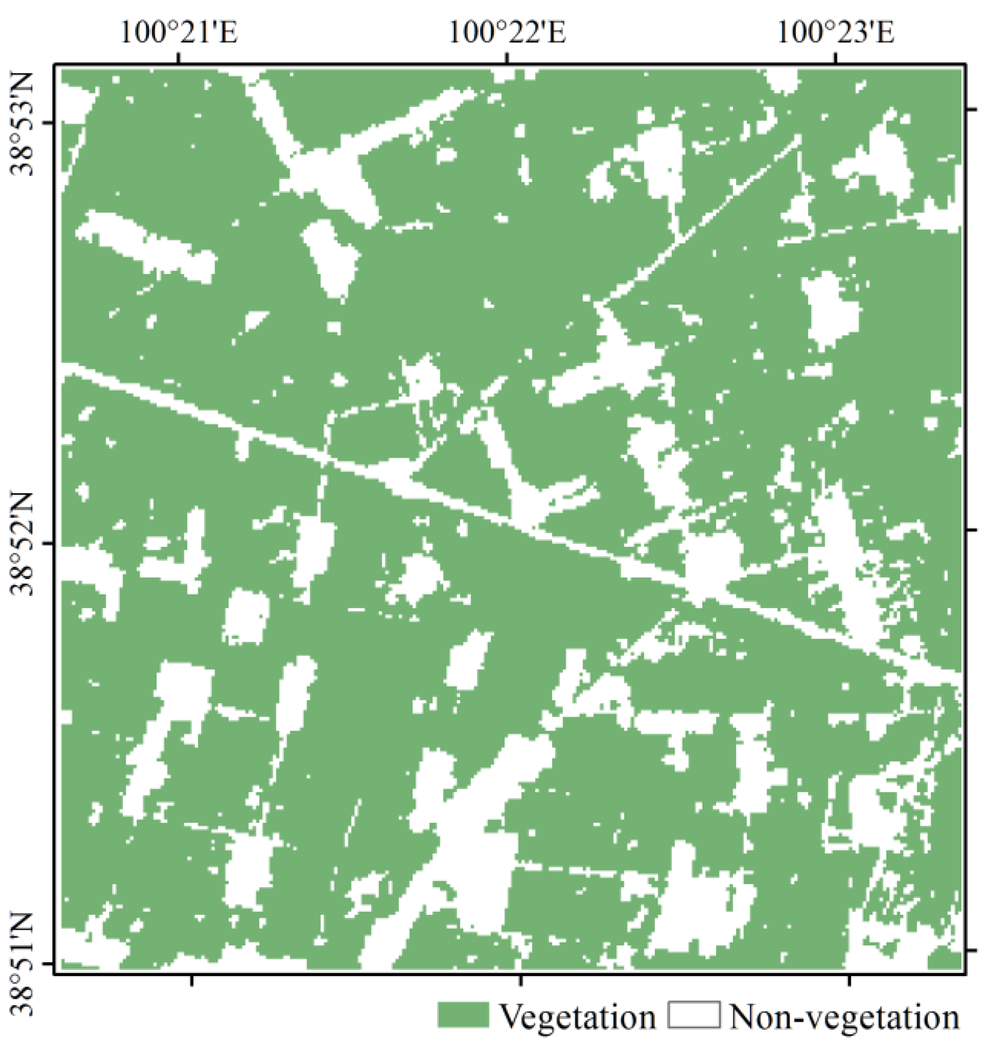
4.1. Extracting the Ancillary Information from High Resolution Images

The proposed method to extract ancillary information from high resolution images was presented in Section 3.1. Decision tree classification was used to distinguish croplands from non-vegetation types including residential areas, irrigation facilities, roads, bare soil, etc. The site comprised 78% cropland and 22% mosaic (or non-vegetation) class in the 4 km × 4 km study area, as shown in Figure 3. The set of test samples, including 1446 vegetation samples and 1785 non-vegetation samples, were used to assess the classification result, showing a high accuracy with overall accuracy of 98% and Kappa coefficient of 0.95 from a confusion matrix. This good performance was partly attributed to the clear and simple spatial structure in 4 km × 4 km region considered.
Figure 3. Land cover map based on ASTER images.
Remotesensing 07 12887 g003
Once the vegetation pixels were identified, the corresponding LAI can be estimated based on the empirical relationship. We calibrated the coefficients of Equation (3) by regression analysis of the relationship between the NDVI and in situ LAI measurements. Forty two sampling points were used to construct the relationship since continuous LAI data at those points were measured from 25 June to 24 August. However, not all field measurements provided complete 10 days of continuous observations, as only part of the collocated ASTER images were acquired during the study period, reducing the amount of data available to derive the empirical relationship. We collated the available ASTER-NDVI values with in situ LAI measurements to establish Equation (3). In summary, 88 pairs of data (each pair comprising one NDVI value and corresponding in situ LAI value) were available. The data were divided into two subsets: 65% of the pairs intended for model calibration and the remainder for independent test. The coefficients of the model were determined by the calibration dataset (a = 4.9, b = 0.89) with R2 = 0.63 showed in Figure 4a. Figure 4b shows that there was minimal scatter between the measured and estimated LAI values, as indicated by the statistical quantities (R2 = 0.52, RMSE = 0.66). The RER of 6.6 indicated that the model had good practical utility.
Figure 4. The constructed empirical relationship: (a) the empirical relationship between LAI and NDVI, (b) Comparison between measured and estimated LAI values.
Remotesensing 07 12887 g004
Once the LAI estimates of vegetation and non-vegetation types were determined, the representative LAI of vegetation surface and reference LAI for the site could be obtained. Figure 5 shows these values distributed over time, with the average value of in situ LAI measurements at the 42 sampling points. Five reference LAI values were distributed separately over time and would be used to evaluate the proposed algorithm. The average LAI agreed well with the representative LAI of vegetation surface and captured the vegetation temporal variation, but marginally represent the LAI over the heterogeneous surface.
Figure 5. The representative LAI of vegetation surface and reference LAI in this site with the average values of in situ LAI measurements.
Remotesensing 07 12887 g005

4.2. Evaluation of the Upscaling Algorithm

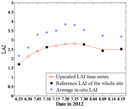
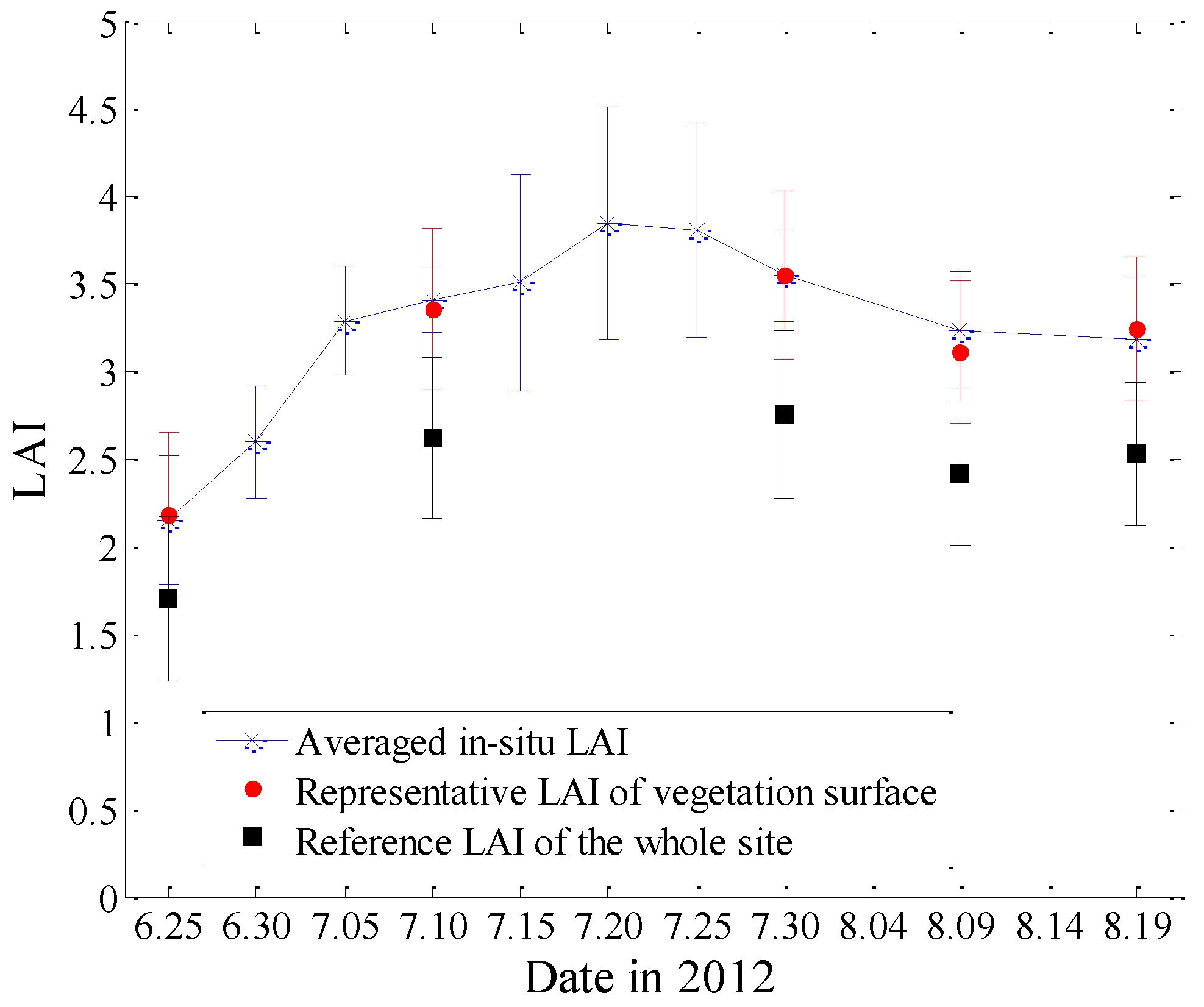
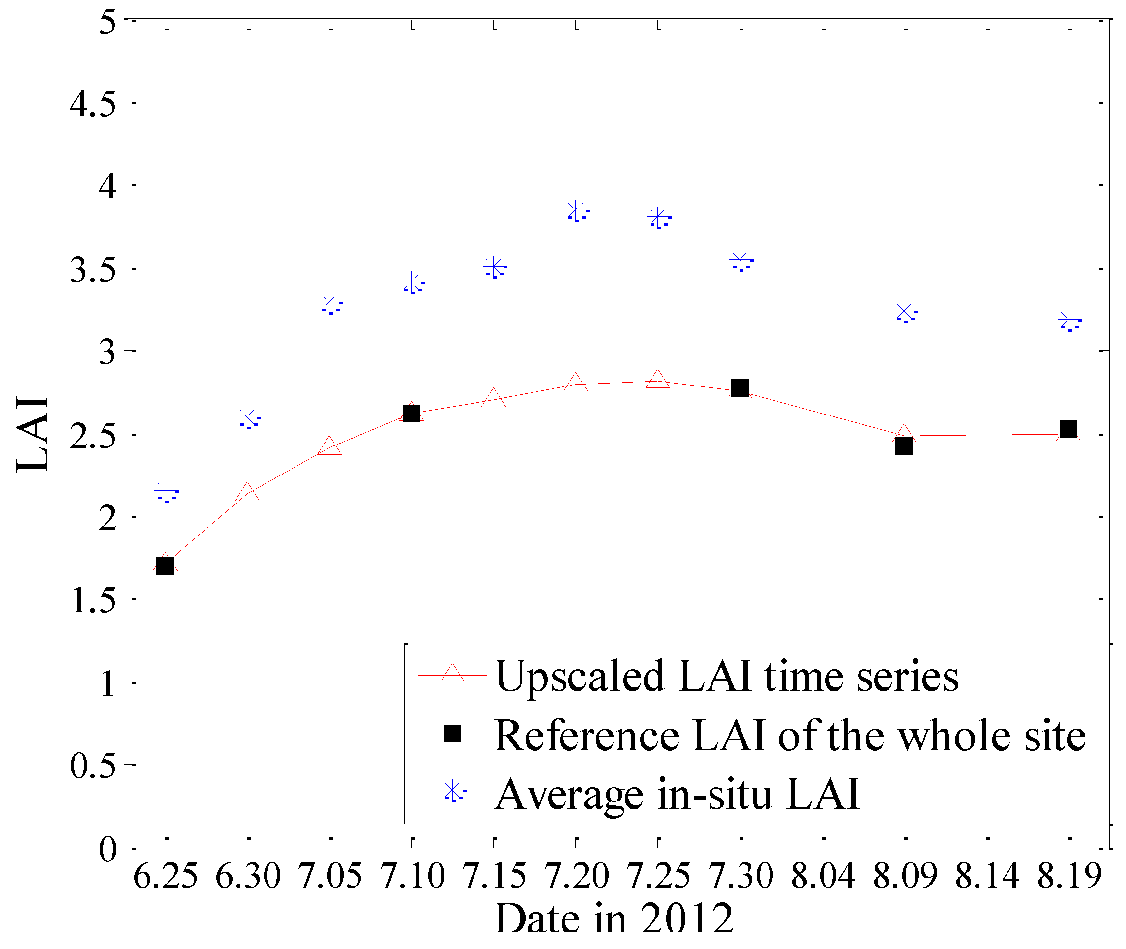
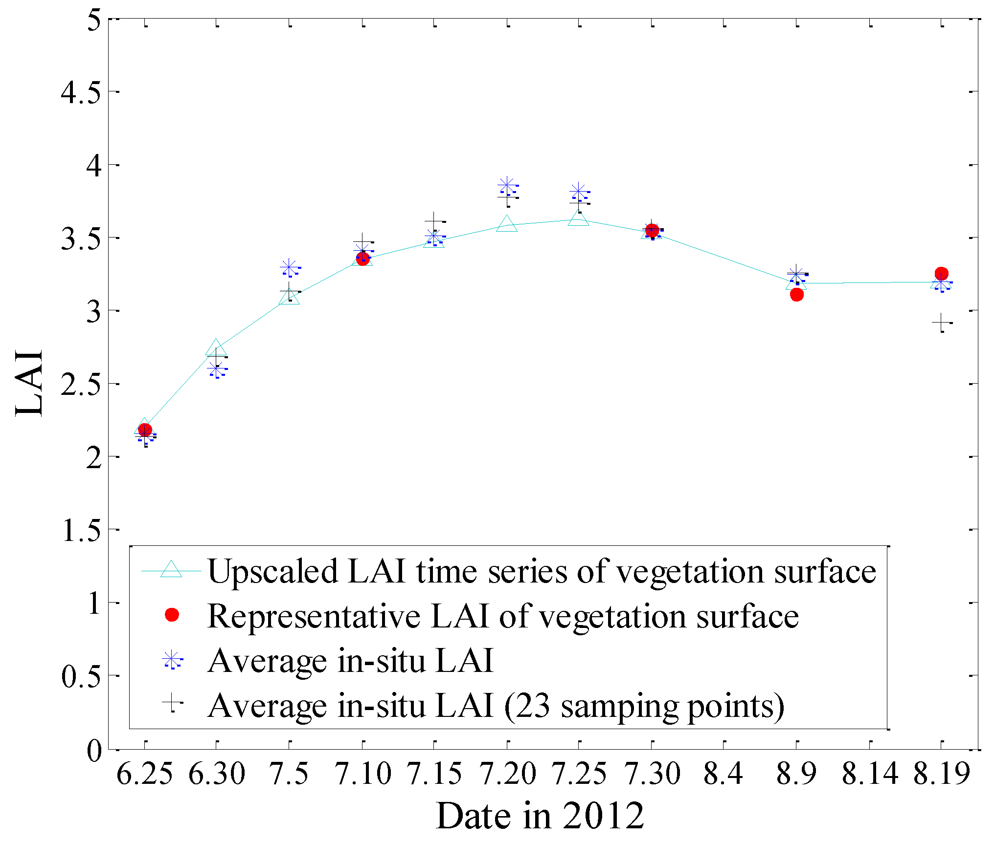
4.2.1. Evaluation of the Upscaled LAI Time Series

We tested the usability of the proposed upscaling algorithm to obtain the ground truth of LAI time series. All data was used for upscaling, including five representative LAI values and the continuous LAI measurements at the 42 sampling points. Since only some of the 42 sampling points presented complete 10 days of continuous observations, we interpolated the in situ measurements using quadratic interpolation [40]. Interpolated values separated by more than five days from an actual measurement were excluded from the analysis. Pooling the measured and interpolated data, 23 sampling points with 10 continuous measurements at each point were available. We applied the upscaling algorithm to these sampling points and compared the upscaled performance with the derived ground truth, as shown in Figure 6.
Figure 6. Upscaled LAI time series and average in situ LAI compared to the reference LAI.
Remotesensing 07 12887 g006
The upscaled LAI time series shows a temporal pattern for the cropland area (red line) in good agreement with the reference LAI (black solid squares) across the entire time period (RMSE = 0.032, n = 23). The average LAI method values are higher than the reference LAI (RMSE = 0.69, n = 42). Thus, averaging in situ LAI measurements does not correctly represent the LAI on a heterogeneous surface, whereas the proposed upscaling method can successfully generate the ground truth of LAI time series with a limited number of in situ LAI measurements (23 in this case).

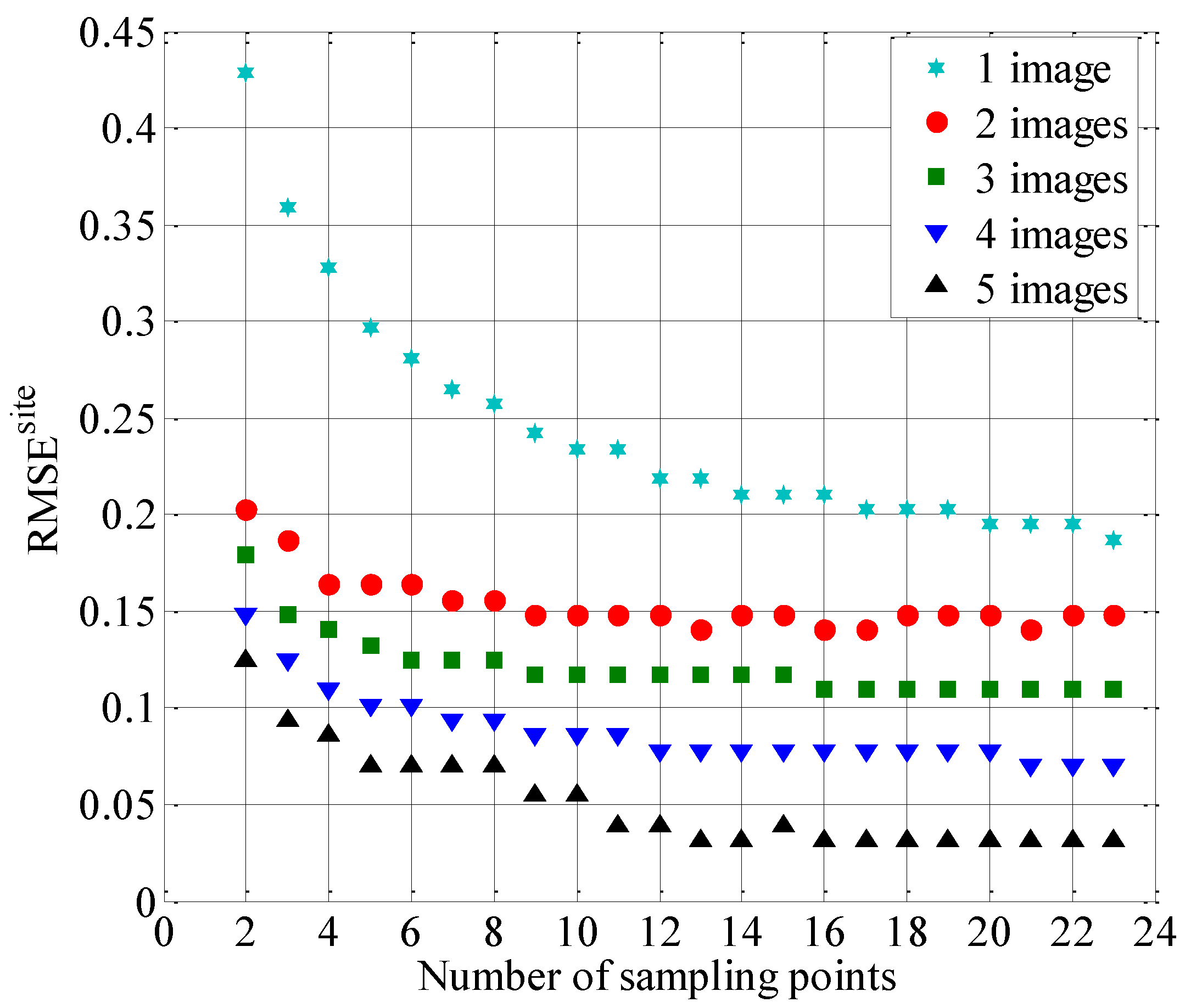
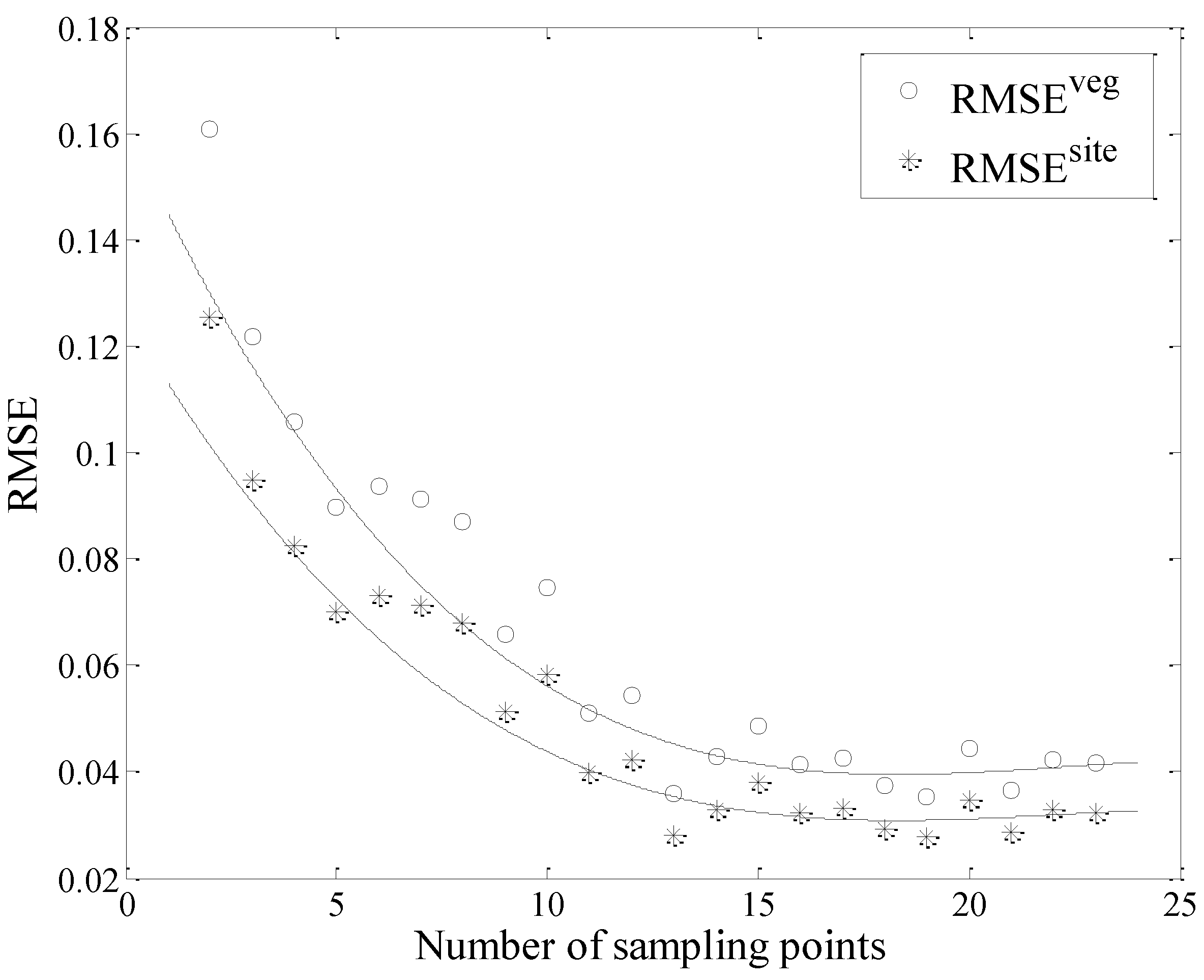
4.2.2. Required Number of Sampling Points

Twenty three sampling points were used to perform the upscaling for this study. However, in practice, there may be only a few sampling points available in the study area. Therefore, we conducted a sensitivity study to define the level of input data that maybe required. The number of sampling points (2–23) were repeatedly randomly sampled from the total points, the upscaling algorithm applied to the sampled points and the mean RMSE values calculated, as shown in Figure 7. The mean RMSE of the upscaled LAI decreases with increasing number of points, but is relatively stable after including 13 sampling points. Thus, the ground truth of LAI can be effectively identified when only a few sampling points are available using the proposed upscaling algorithm.
Figure 7. Upscaled performances with the number of sampling points.
Remotesensing 07 12887 g007
Figure 8. Upscaled LAI time series of vegetation surface, average in situ LAI and representative LAI of vegetation surface.
Remotesensing 07 12887 g008
We further analyzed the upscaled LAI performance of the vegetation surface, which was the essential intermediate result of upscaling, as shown in Figure 8. The upscaled LAI was more consistent with the corresponding representative LAI (red solid circles) (RMSE = 0.041, n = 23) than the average LAI (RMSE = 0.17, n = 23). The measured field LAI data was also able to represent the vegetation surface features well (RMSE = 0.069, n = 42). The proposed upscaling method provides a similar performance with less sampling points (RMSE = 0.07, n = 8, Figure 7), and increasing the sampling points does significantly improve the performance. This may benefit field experiment by reducing labor and instrument costs, and extend the usefulness of existing datasets currently without sufficient measurements for conventional LAI analysis.

4.2.3. Number of High Resolution Images

Another important issue for the proposed upscaling algorithm is the availability of the high resolution remote sensing data. As discussed above, this data normally has low temporal resolution and is also often contaminated by clouds, leading to the unavailability of representative LAI of the vegetation surface for upscaling. We analyzed proposed upscaling algorithm performance with different numbers of ASTER images (1–5) and evaluated the resultant LAIs against the five derived reference LAI values, as shown in Figure 9. The mean RMSEs were calculated following the procedures detailed above.
The mean RMSE decreased with increasing number of images for any number of sampling points. For a given number of images, increasing the sampling points for upscaling could improve the performance, suggesting that the in situ LAI data and images can compensate each other to achieve a satisfactory result. Zhang et al. [55] suggested the characteristic accuracy of LAI ranges from 0.1 to 0.6, varying with the spatial scale. If RMSE of 0.15 was required, only two images and nine sampling points would be sufficient to obtain the corresponding ground truth of the LAI time series.
Figure 9. Upscaled LAI performance with the number of ASTER images and sampling points
Remotesensing 07 12887 g009

4.3. Comparison with LAI Products

The proposed ground truth of LAI time series with 23 sampling points were used to investigate the temporal performance of LAI products. The average value of in situ LAI measurements was also used for comparison.

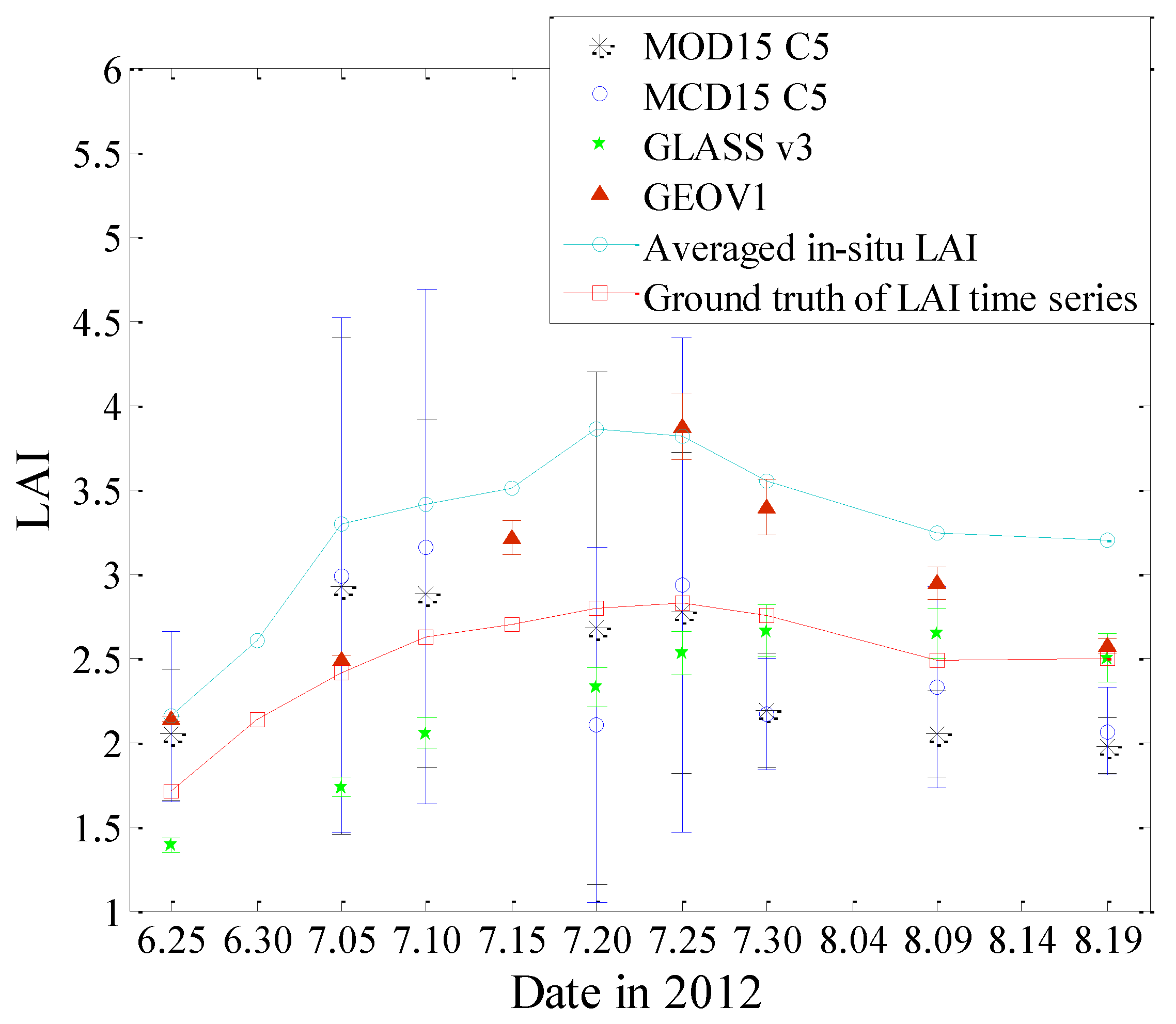
4.3.1. Time Series Analysis

Figure 10 shows the temporal trajectory of different LAI products across the site during the study period, compared with the ground truth of LAI calculated by our proposed method, and the average in situ LAI. The satellite products were generally in better agreement with the ground truth than the average in situ LAI.
LAI estimates from GLASS and GEOV1 show a smooth temporal pattern, but systematically lower and higher than the ground truth, respectively. Overestimation of GEOV1 over cropland biomes has also been found by Claverie et al. [34]. In addition, GLASS LAI tended to increase later than GEOV1 and in situ LAI measurements, which approximately peaked between mid to end of July. The two MODIS C5 collections agreed very well, overlapping for much of the time, but exhibited some temporal discontinuity and an unrealistically variability with higher deviations, especially in the fast growing season. This may be due to the impact of cloud cover or the LAI derivation method for those datasets [15].
Figure 10. Time series comparison between ground truth of LAI and average in situ LAI for the 4 km × 4 km area and corresponding LAI products
Remotesensing 07 12887 g010

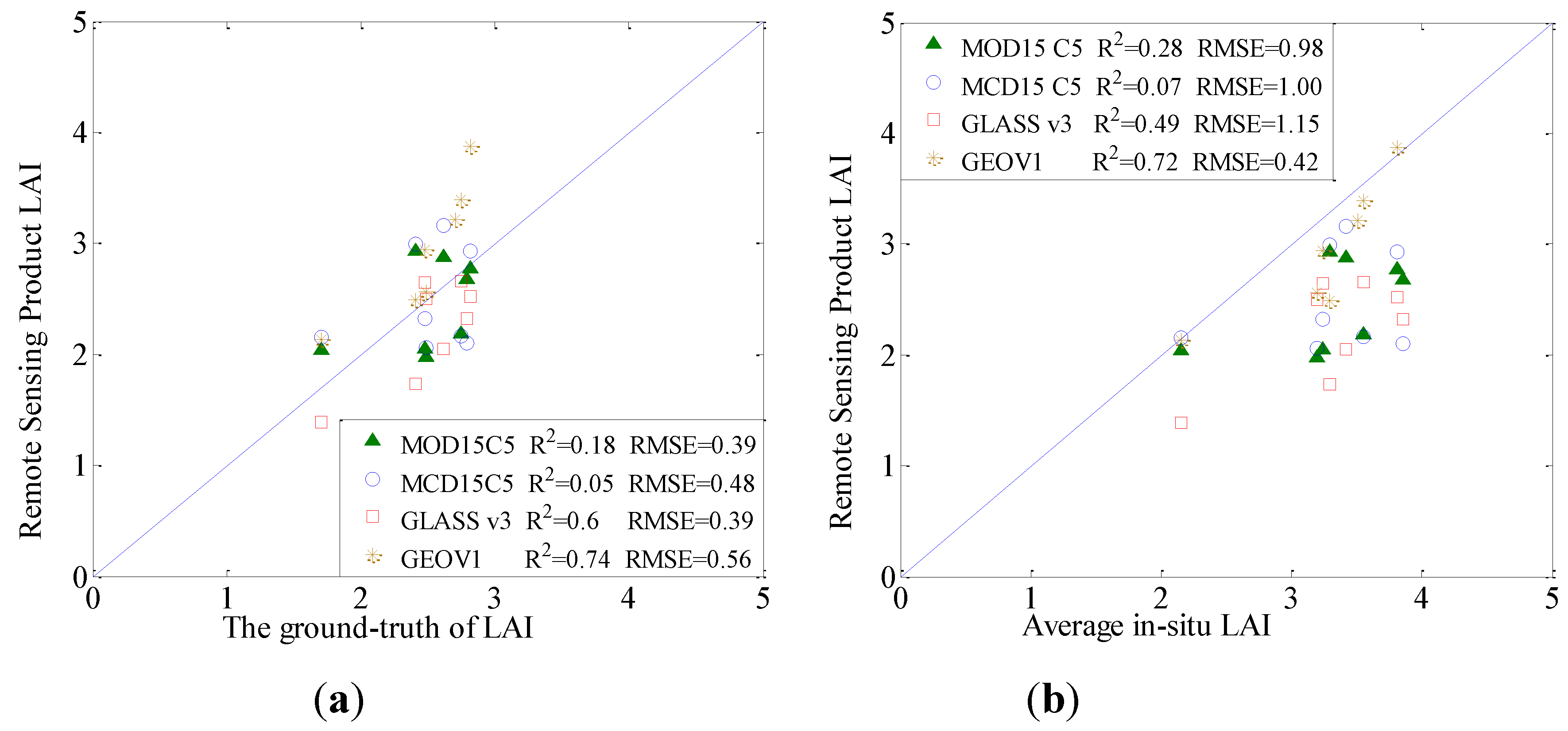
4.3.2. Direct Comparison

Figure 11a shows MOD15 C5 and GLASS agreed reasonably well with ground truth of LAI (RMSE = 0.39 for both products). However, GLASS appeared to be underestimation by a small amount. The superiority of the Terra + Aqua combined MCD15 C5 product (RMSE = 0.48) was not as expected from previous studies [15], which could be partly attributed to there being no quality flag applied. GEOV1 displayed systematic overestimation for LAI (RMSE = 0.56), which was consistent with earlier results [34].
When compared to the average in situ LAI, the uncertainty (RMSE > 0.98) for most products were significantly larger than for the proposed upscaled LAI, except for GEOV1 (Figure 11b). The large uncertainty could be a result of the different scale between the field measurements and the remote sensing products due to the surface heterogeneity, which produces some errors and biases. Thus, an appropriate upscaling method is vital and has been particularly recommended for validation studies [14].
Figure 11. Scatter plots comparing (a) ground truth LAI and (b) average in situ LAI to corresponding MOD15 C5, MCD15 C5, GLASS, and GEOV1 LAI in the 4 km × 4 km area
Remotesensing 07 12887 g011

5. Discussion

The major issue facing the validation of LAI products is the spatial mismatch between ground measurements and medium resolution remote sensing LAI products, due to the heterogeneous land surface. This is why the bridging method based on high spatial remote sensing images is commonly chosen for validation [14]. However, it remains a challenging task to obtain the ground truth of LAI time series across a wide range of sites. Several studies suggest that WSN technology has significant advantages for ground validation and is able to acquire data automatically in large areas over long periods [40]. In this study, we proposed an upscaling algorithm to obtain the representative ground truth of LAI time series from in situ LAI data measured by WSN observation system. The algorithm was evaluated using a dataset collected over a 4 km × 4 km study area composed of cropland and various non-vegetation types in the Yingke irrigation district. The results indicated our algorithm can be successfully applied to this heterogeneous cropland area.
Previous studies have suggested that ancillary information can support upscaling of in situ measurements, especially when only a limited number of sampling points are available over a large area [14,41]. The bridging method, for example, is based on the use of high spatial resolution images to extend ground sampling measurements. In our proposed algorithm, we also incorporate ancillary information extracted from high spatial resolution image to support upscaling. However, the proposed algorithm requires less images than the bridging method and provides better ground truth outcomes. Ten temporally continuous ground truth of LAI from June to August were obtained by our proposed method, whereas only five were acquired by the bridging method. Increasing the sampling points in our proposed algorithm can reduce the image requirement for upscaling. For the case studied, ground truth of the LAI time series with high accuracy (RMSE = 0.15) could be obtained with two images and nine sampling points.
The EM algorithm is considered to be a simple and robust tool for parameter estimation in models with incomplete data [46,47,48], and we employed it to compute the optimal weight of the in situ LAI measurement in the study area. The EM algorithm was robust even when the number of parameters was much larger than that of observed data. For example, a weight vector for the 23 sampling points can be accurately derived using the data from just five dates. Moreover, the different weights of in situ measurements were able to identify the spatial differences of vegetation growth and facilitate a satisfactory result using a limited number of sampling points. The proposed upscaled LAI using eight sampling points described the representative LAI of vegetation surface well (RMSE = 0.07, n = 8), which was very similar to the performance of the average value of 42 in situ LAI measurements (RMSE = 0.069, n = 42). This may facilitate field work and analysis of existing ground data currently without sufficient sampling points. In this study, the weights were limited to be constant during the study period based on the assumption that spatial pattern of vegetation growth was not changing with time. However, the weight may change with time due to the temporal change of spatial pattern of vegetation growth. We will investigate the method to determine the weight varying with time in the future work.
The simple averaging method is restricted to relatively homogeneous surfaces with sufficient ground measurements [15]. Our study showed that the average LAI of in situ measurements did not agree well with the representative LAI of the whole heterogeneous site (RMSE = 0.69, n = 42). If this value was regarded as ground truth to validate LAI products, it would produce significant bias upon validation. In our proposed upscaling algorithm, the spatial heterogeneity across the site was explicitly considered based on land cover types, making the algorithm suitable for heterogeneous surfaces (RMSE = 0.032, n = 23). Previous studies have reported that information relating to land cover type is commonly used in scaling issues [49,50,51,52].
The regression method has been widely used to estimate the high-resolution LAI image and generally produces a good result with sufficient observations [16,18,19,20,21,22,23]. However, previous study has found that some compression of the variance or error of LAI estimates generally presented in the empirical relationship [21]. In this study, this method was applied to build the empirical relationship between the in situ LAI measurements and corresponding NDVI. The data covering several dates were used and able to ensure the quantity and variation of observations. The evaluated result shows that good estimates were achieved for LAI (R2 = 0.52, RMSE = 0.66) and the RER of 6.6 indicated that the model had good practical utility. Figure 4b shows that the low LAI was overestimated slightly while high LAI was underestimated. However, this error had little effect on our study, since the LAI were mostly distributed from two to four, and the overestimated and underestimated LAI values were counterbalanced during the averaging process. This was revealed by the clear distinction between the results of Figure 11a (ground truth LAI compared with LAI products) and Figure 11b (average in situ LAI compared with LAI products).
Compared with the ground truth of LAI over site, MOD15 C5 shows a good consistency on cropland (RMSE = 0.39, n = 8), which agrees with findings (RMSE = 0.229, n = 105) reported recently by Claverie et al. [34] using the bridging method. However, MOD15 C5 shows unrealistic variability, especially during the fast growing season, a drawback also indicated by Fang et al. [15]. The Terra + Aqua combined MCD15 C5 shows marginal improvement, partly affected by ignoring quality flag information. The latest GEOV1 and GLASS show smooth temporal trajectories [11,12], but GEOV1 overestimates representative LAI, similar to previous findings with the bridging method [11,34].

6. Conclusions

In this study, a two-step upscaling algorithm was proposed to obtain the representative ground truth of LAI time series in heterogeneous surfaces based on in situ LAI data measured by the WSN observation system. The representative LAI time series of the vegetation surface was acquired by optimal weighted combination of the in situ LAI measurements at several sampling points, and then the ground truth of LAI over the whole site could be calculated by area weighted merging of the representative LAIs of different land cover types. Emphasis was given to determining the optimal weight based on the consideration of the spatial differences of vegetation growth, and calculated using the EM algorithm constrained by ancillary information extracted from high resolution images and concurrent in situ measurements.
The proposed upscaling algorithm was evaluated, showing that the algorithm can be successfully applied to heterogeneous land surfaces, even with a limited number of sampling points distributed across the site. The upscaled LAI time series can be obtained and agrees well with the ground truth of LAI (RSME = 0.032, n = 23). The proposed upscaled LAI of the vegetation surface with few sampling points can represent the corresponding representative LAI (RMSE = 0.07, n = 8), which was consistent to the average values of multiple LAI measurements (RMSE = 0.069, n = 42).
The proposed ground truth LAI time series was compared with four LAI products. In general, the latest LAI retrievals from GEOV1 and GLASS showed a smooth temporal trajectory, but tended to a slight bias for this site. While MOD15 C5 showed better consistency with the proposed ground truth LAI than MCD15 C5, both showed unrealistic variability.
Our study investigated the potential of the ground measurements using the WSN observation system for the validation of LAI products over a crop site in the Heihe River basin. The proposed upscaling algorithm can be applied to other land cover types, where a network of sampling points and continuous measurements exists.

Acknowledgements

This research was supported by the National Basic Research Program of China under grant No. 2013CB733403, and the National Natural Science Foundation of China under grant No. 41171263.

Author Contributions

Yuechan Shi designed the framework of this research work and wrote the manuscript; Jindi Wang gave important guidance on the work and checked the writing; Jun Qin offered support for the optimization algorithm and Yonghua Qu provided the field data.

Conflicts of Interest

The authors declare no conflict of interest.

References

  1. Chen, J.M.; Black, T.A. Defining leaf area index for non-flat leaves. Plant Cell Environ. 1992, 15, 421–429. [Google Scholar] [CrossRef]
  2. Moulin, S.; Bondeau, A.; Delecolle, R. Combining agricultural crop models and satellite observations: From field to regional scales. Int. J. Remote Sens. 1998, 19, 1021–1036. [Google Scholar] [CrossRef]
  3. Running, S.W.; Baldocchi, D.D.; Turner, D.P.; Gower, S.T.; Bakwin, P.S.; Hibbard, K.A. A global terrestrial monitoring network integrating tower fluxes, flask sampling, ecosystem modeling and EOS satellite data. Remote Sens. Environ. 1999, 70, 108–127. [Google Scholar] [CrossRef]
  4. Turner, D.P.; Cohen, W.B.; Kennedy, R.E.; Fassnacht, K.S.; Briggs, J.M. Relationships between leaf area index, FAPAR and net primary production of terrestrial ecosystems. Remote Sens. Environ. 1999, 70, 52–68. [Google Scholar] [CrossRef]
  5. Zhang, P.; Anderson, B.; Tan, B.; Huang, D.; Myneni, R. Potential monitoring of crop production using a satellite-based Climate-Variability Impact Index. Agric. For. Meteorol. 2005, 132, 344–358. [Google Scholar] [CrossRef]
  6. Dickinson, R.E. Land processes in climate models. Remote Sens. Environ. 1995, 51, 27–38. [Google Scholar] [CrossRef]
  7. Sellers, P.J.; Dickinson, R.E.; Randall, D.A.; Betts, A.K.; Hall, F.G.; Berry, J.A.; Collatz, G.J.; Denning, A.S.; Mooney, H.A.; Nobre, C.A.; et al. Modeling the exchange of energy, water, and carbon between continents and atmosphere. Science 1997, 275, 502–509. [Google Scholar] [CrossRef] [PubMed]
  8. Arora, V. Modeling vegetation as a dynamic component in soil-vegetation-atmosphere transfer schemes and hydrological models. Rev. Geophys. 2002, 40, 1–26. [Google Scholar] [CrossRef]
  9. Liang, S.L.; Li, X.W.; Wang, J.D. Leaf area index. In Advanced Remote Sensing: Terrestrial Information Extraction and Applications; Science Press: Beijing, China, 2012; Volume 11, pp. 342–344. [Google Scholar]
  10. Myneni, R.B.; Hoffman, S.; Knyazikhin, Y.; Privette, J.L.; Glassy, J.; Tian, Y.; Wang, Y.; Song, X.; Zhang, Y.; Smith, G.R.; et al. Global products of vegetation leaf area and fraction absorbed PAR from year one of MODIS data. Remote Sens. Environ. 2002, 83, 214–231. [Google Scholar] [CrossRef]
  11. Baret, F.; Weiss, M.; Lacaze, R.; Camacho, F.; Makhmara, H.; Pacholcyzk, P.; Smets, B. GEOV1: LAI, FAPAR essential climate variables and FCOVER global time series capitalizing over existing products. Part1: Principles of development and production. Remote Sens. Environ. 2013, 137, 299–309. [Google Scholar] [CrossRef]
  12. Xiao, Z.Q.; Liang, S.L.; Wang, J.D.; Chen, P.; Yin, X.; Zhang, L.; Song, J.L. Use of general regression neural networks for generating the GLASS leaf area index product from time-series MODIS surface reflectance. IEEE Trans. Geosci. Remote Sens. 2014, 52, 209–223. [Google Scholar] [CrossRef]
  13. Justice, C.; Belward, A.; Morisette, J.; Lewis, P.; Privette, J.; Baret, F. Developments in the validation of satellite sensor products for the study of the land surface. Int. J. Remote Sens. 2000, 21, 3383–3390. [Google Scholar] [CrossRef]
  14. Morisette, J.T.; Baret, F.; Privette, J.L.; Myneni, R.B.; Nickeson, J.E.; Garrigues, S.; Shabanov, N.V.; Weiss, M.; Fernandes, R.A.; Leblanc, S.G.; et al. Validation of global medium-resolution LAI Products: A framework proposed within the CEOS Land Product Validation subgroup. IEEE Trans. Geosci. Remote Sens. 2006, 44, 1804–1817. [Google Scholar] [CrossRef]
  15. Fang, H.L.; Wei, S.; Liang, S.L. Validation of MODIS and CYCLOPES LAI products using global field measurement data. Remote Sens. Environ. 2012, 119, 43–54. [Google Scholar] [CrossRef]
  16. Baret, F.; Weiss, M.; Garrigue, S.; Allard, D.; Leroy, M.; Jeanjean, H.; Fernandes, R.; Myneni, R.B.; Morisette, J.T.; Privette, J.; et al. VALERI: A Network of Sites and a Methodology for the Validation of Medium Spatial Resolution Satellite Products. Remote Sens. Environ. 2015. submitted. [Google Scholar]
  17. Campbell, J.L.; Burrows, S.; Gower, S.T.; Cohen, W.B. BigFoot: Characterizing land cover, LAI, and NPP at the landscape scale for EOS/MODIS validation. In Field Manual, 2.1st ed.Environmental Sciences Division Publication 4937; Oak Ridge National Laboratory: Oak Ridge, TN, USA, 1999; pp. 29–429. [Google Scholar]
  18. Weiss, M.; de Beaufort, L.; Baret, F.; Allard, D.; Bruguier, N.; Marloie, O. Mapping leaf area index measurements at different scales for the validation of large swath satellite sensors: First results of the VALERI project. In Proceedings of the 8th International Symposium in Physical Measurements and Remote Sensing, Aussois, France, 8–12 January 2001; pp. 125–130.
  19. Chen, J.M.; Pavlic, G.; Brown, L.; Cihlar, J.; Leblanc, S.G.; White, H.P.; Hall, R.J.; Peddle, D.R.; King, D.J.; Trofymow, J.A.; et al. Derivation and validation of Canada-wide coarse-resolution leaf area index maps using high-resolution satellite imagery and ground measurements. Remote Sens. Environ. 2002, 80, 165–184. [Google Scholar] [CrossRef]
  20. Fernandes, R.; Butson, C.; Leblanc, S.G.; Latifovic, R. Landsat-5 TM and Landsat-7 ETM+ based accuracy assessment of leaf area index products for Canada derived from SPOT-4 VEGETATION data. Can. J. For. Res. 2003, 29, 241–258. [Google Scholar] [CrossRef]
  21. Cohen, W.B.; Maiersperger, T.K.; Gower, S.T.; Turner, D.P. An improved strategy for regression of biophysical variables and Landsat ETM+ data. Remote Sens. Environ. 2003, 84, 561–571. [Google Scholar] [CrossRef]
  22. Cohen, W.B.; Maiersperger, T.K.; Yang, Z.Q.; Gower, S.T.; Turner, D.P.; Ritts, W.D.; Berterretche, M.; Running, S.W. Comparisons of land cover and LAI estimates derived from ETM+ and MODIS for four sites in North America: A quality assessment of 2000/2001 provisional MODIS products. Remote Sens. Environ. 2003, 88, 233–255. [Google Scholar] [CrossRef]
  23. Cohen, W.B.; Maiersperger, T.K.; Turner, D.P.; Ritts, W.D.; Pflugmacher, D.; Kennedy, R.E.; Kirschbaum, A.; Running, S.W.; Costa, M.; Gower, S.T. MODIS Land Cover and LAI Collection 4 product quality across nine sites in the western hemisphere. IEEE Trans. Geosci. Remote Sens. 2006, 44, 1843–1857. [Google Scholar] [CrossRef]
  24. Tan, B.; Hu, J.; Zhang, P.; Huang, D.; Shabanov, N.; Weiss, M.; Knyazikhin, Y.; Myneni, R.B. Validation of Medium Resolution Imaging Spectroradiometer leaf area index product in croplands of Alpilles, France. J. Geophys. Res. 2005, 110, 1–15. [Google Scholar]
  25. Yang, W.Z.; Tan, B.; Huang, D.; Rautiniainen, M.; Shabanov, N.V.; Wang, Y.; Privette, J.L.; Huemmrich, K.F.; Fensholt, R.; Sandholt, I.; et al. MODIS leaf area index products: From validation to algorithm improvement. IEEE Trans. Geosci. Remote Sens. 2006, 44, 1885–1898. [Google Scholar] [CrossRef]
  26. Weiss, M.; Baret, F.; Smith, G.J.; Jonckheere, I.; Coppin, P. Review of methods for in situ leaf area index (LAI) determination: Part II. Estimation of LAI, errors and sampling. Agric. For. Meteorol. 2004, 121, 37–53. [Google Scholar] [CrossRef]
  27. Garrigues, S.; Lacaze, R.; Baret, F.; Morisette, J.T.; Weiss, M.; Nickeson, J.E.; Fernandes, R.; Plummer, S.; Shabanov, N.V.; Myneni, N.V.; et al. Validation and intercomparison of global Leaf Area Index products derived from remote sensing data. J. Geophys. Res. 2008, 113, 1–20. [Google Scholar] [CrossRef]
  28. Weiss, M.; Baret, F.; Garrigues, S.; Lacaze, R. LAI and fAPAR CYCLOPES global products derived from VEGETATION. Part 2: Validation and comparison with MODIS collection 4 products. Remote Sens. Environ. 2007, 110, 317–331. [Google Scholar] [CrossRef]
  29. Camacho, F.; Cernicharo, J.; Lacaze, R.; Baret, F.; Weiss, M. GEOV1: LAI, FAPAR essential climate variables and FCOVER global time series capitalizing over existing products. Part 2: Validation and intercomparison with reference products. Remote Sens. Environ. 2013, 137, 310–329. [Google Scholar] [CrossRef]
  30. Weiss, M.; Baret, F.; Block, T.; Koetz, B.; Burini, A.; Scholze, B.; Lecharpentier, P.; Brockmann, C.; Fernandes, R.; Plummer, S.; et al. On Line Validation Exercise (OLIVE): A web based service for the validation of medium resolution land products. Application to FAPAR products. Remote Sens. 2014, 6, 4190–4216. [Google Scholar] [CrossRef]
  31. Fernandes, R.; Plummer, S.; Nightingale, J. Global Leaf Area Index Product Validation Good Practices; CEOS Working Group on Calibration and Validation-Land Product Validation Sub-Group, 2nd ed. Available online: http://lpvs.gsfc.nasa.gov/LAI_home.html (accessed on 8 July 2015).
  32. Verger, A.; Baret, F.; Camacho, F. Optimal modalities for radiative transfer-neural network estimation of canopy biophysical characteristics: Evaluation over an agricultural area with CHRIS/PROBA observations. Remote Sens. Environ. 2011, 115, 415–426. [Google Scholar] [CrossRef]
  33. Duveiller, G.; Weiss, M.; Baret, F.; Defourny, P. Retrieving wheat Green Area Index during the growing season from optical time series measurements based on neural network radiative transfer inversion. Remote Sens. Environ. 2011, 115, 887–896. [Google Scholar] [CrossRef]
  34. Claverie, M.; Vermote, E.F.; Weiss, M.; Baret, F.; Hagolle, O.; Demarez, V. Validation of coarse spatial resolution LAI and FAPAR time series over cropland in southwest France. Remote Sens. Environ. 2013, 139, 216–230. [Google Scholar] [CrossRef]
  35. Ganguly, S.; Nemani, R.R.; Zhang, G.; Hashimoto, H.; Milesi, C.; Michaelis, A.; Wang, W.L.; Votava, P.; Samanta, A.; Melton, F.; et al. Generating global leaf area index from Landsat: Algorithm formulation and demonstration. Remote Sens. Environ. 2012, 122, 185–202. [Google Scholar] [CrossRef]
  36. Di, L.P.; Karen, M.; Terence, L.V.Z. Earth observation sensor web: An overview. IEEE J. Sel. Top. Appl. Earth Obs. Remote Sens. 2010, 3, 415–417. [Google Scholar] [CrossRef]
  37. Moghaddam, M.; Entekhabi, D.; Goykhman, Y.; Li, K.; Liu, M.Y.; Mahajan, A.; Nayyar, A.; Shuman, D.; Teneketzis, D. A wireless soil moisture smart sensor web using physics-based optimal control: Concept and initial demonstrations. IEEE J. Sel. Top. Appl. Earth Obs. Remote Sens. 2010, 3, 522–535. [Google Scholar] [CrossRef]
  38. Bauer, J.; Siegmann, B.; Jarmer, T.; Aschenbruck, N. On the potential of Wireless Sensor Networks for the in-field assessment of bio-physical crop parameters. In Proceedings of 2014 IEEE 39th Conference on the Local Computer Networks Workshops, Edmonton, AB, Canada, 8–11 September 2014; pp. 523–530.
  39. Qu, Y.H.; Wang, J.D.; Dong, J.; Jiang, F.B. Design and experiment of crop structural parameters automatic measurement system. Trans. CSAE. 2012, 28, 160–165. (In Chinese) [Google Scholar]
  40. Qu, Y.H.; Zhu, Y.Q.; Han, W.C.; Wang, J.D.; Ma, M.G. Crop leaf area index observations with a wireless sensor network and its potential for validating remote sensing products. IEEE J. Sel. Top. Appl. Earth Obs. Remote Sens. 2014, 7, 431–444. [Google Scholar] [CrossRef]
  41. Qin, J.; Yang, K.; Lu, N.; Chen, Y.Y.; Zhao, L.; Han, M.L. Spatial upscaling of in situ soil moisture measurements based on MODIS derived apparent thermal inertia. Remote Sens. Environ. 2013, 138, 1–9. [Google Scholar] [CrossRef]
  42. Li, X.; Cheng, G.; Liu, S.; Xiao, Q.; Ma, M.; Jin, R.; Che, T.; Liu, Q.; Wang, W.; Qi, Y. Heihe watershed allied telemetry experimental research (HiWATER): Scientific objectives and experimental design. Bull. Am. Meteorol. Soc. 2013, 94, 1145–1160. [Google Scholar] [CrossRef]
  43. Qu, Y.H.; Zhu, Y.Q.; Han, W.C. HiWATER: Dataset of LAINet Observations in the Middle Reaches of the Heihe River Basin; Institute of Remote Sensing Applications, Beijing Normal University Press: Beijing, China, 2012. [Google Scholar]
  44. Gu, J.; Congalton, R.G.; Pan, Y. The impact of positional errors on soft classification accuracy assessment: A simulation analysis. Remote Sens. 2015, 7, 579–599. [Google Scholar] [CrossRef]
  45. Yang, W.; Shabanov, N.V.; Huang, D.; Wang, W.; Dickinson, R.E.; Nemani, R.R.; Knyazikhin, Y.; Myneni, R.B. Analysis of leaf area index products from combination of MODIS Terra and Aqua data. Remote Sens. Environ. 2006, 104, 297–312. [Google Scholar] [CrossRef]
  46. Páscoa, R.N.M.J.; Machado, S.; Magalhães, L.M.; João, A.L. Value adding to red grape pomace exploiting eco-friendly FT-NIR spectroscopy technique. Food Bioprocess Tech. 2015, 8, 865–874. [Google Scholar] [CrossRef]
  47. De, G.A.; Lippolis, V.; Nordkvist, E.; Visconti, A. Rapid and non-invasive analysis of deoxynivalenol in durum and common wheat by Fourier-transform near infrared (FT-NIR) spectroscopy. Food Addit. Contam. 2009, 26, 907–917. [Google Scholar]
  48. Dellaert, F. The Expectation Maximization Algorithm; Technical Report GIT-GVU-02-20; Georgia Institute of Technology: Savannah, GA, USA, 2002. [Google Scholar]
  49. Chen, J.M. Spatial scaling of a remotely sensed surface parameter by contexture. Remote Sens. Environ. 1999, 69, 30–42. [Google Scholar] [CrossRef]
  50. Jin, Z.; Tian, Q.; Chen, J.M.; Chen, M. spatial scaling between leaf area index maps of different resolutions. J. Environ. Manage. 2007, 85, 628–637. [Google Scholar] [CrossRef] [PubMed]
  51. Tian, Y.H.; Woodcock, C.E.; Wang, Y.J.; Privette, J.L.; Shabanov, N.V.; Zhou, L.M.; Buermann, W.; Dong, J.R.; Veikkanen, B.; et al. Multiscale analysis and validation of the MODIS LAI product: I. Uncertainty assessment. Remote Sens. Environ. 2002, 83, 414–430. [Google Scholar] [CrossRef]
  52. Hufkens, K.; Bogaert, J.; Dong, Q.H.; Lud, L.; Huang, C.L.; Mad, M.G.; Che, T.; Li, X.; Veroustraete, F.; Ceulemans, R. Impacts and uncertainties of upscaling of remote-sensing data validation for a semi-arid woodland. J. Arid. Environ. 2008, 72, 1490–1505. [Google Scholar] [CrossRef]
  53. Blume, M. Expectation Maximization: A Gentle Introduction; Technical University of Munich-Institute for Computer Science Press: Munich, Germany, 2002. [Google Scholar]
  54. Do, C.B.; Batzoglou, S. What is the expectation maximization algorithm? Nat. Biotechnol. 2008, 26, 897–899. [Google Scholar] [CrossRef] [PubMed]
  55. Zhang, R.H.; Tian, J.; Li, Z.L.; Su, H.B.; Chen, S.H. Principles and methods for the validation of quantitative remote sensing products. Sci. China Ser. Earth D. 2010, 40, 211–222. [Google Scholar] [CrossRef]

