How Reliable is the MODIS Land Cover Product for Crop Mapping Sub-Saharan Agricultural Landscapes?


Abstract
: Accurate cropland maps at the global and local scales are crucial for scientists, government and nongovernment agencies, farmers and other stakeholders, particularly in food-insecure regions, such as Sub-Saharan Africa. In this study, we aim to qualify the crop classes of the MODIS Land Cover Product (LCP) in Sub-Saharan Africa using FAO (Food and Agricultural Organisation) and AGRHYMET (AGRiculture, Hydrology and METeorology) statistical data of agriculture and a sample of 55 very-high-resolution images. In terms of cropland acreage and dynamics, we found that the correlation between the statistical data and MODIS LCP decreases when we localize the spatial scale (from R2 = 0.86 *** at the national scale to R2 = 0.26 *** at two levels below the national scale). In terms of the cropland spatial distribution, our findings indicate a strong relationship between the user accuracy and the fragmentation of the agricultural landscape, as measured by the MODIS LCP; the accuracy decreases as the crop fraction increases. In addition, thanks to the Pareto boundary method, we were able to isolate and quantify the part of the MODIS classification error that could be directly linked to the performance of the adopted classification algorithm. Finally, based on these results, (i) a regional map of the MODIS LCP user accuracy estimates for cropland classes was produced for the entire Sub-Saharan region; this map presents a better accuracy in the western part of the region (43%–70%) compared to the eastern part (17%–43%); (ii) Theoretical user and producer accuracies for a given set of spatial resolutions were provided; the simulated future Sentinel-2 system would provide theoretical 99% user and producer accuracies given the landscape pattern of the region.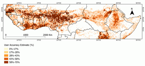
1. Introduction
When addressing food security issues, accurate mapping of cropland at both global and local scales is crucial for scientists, government and nongovernment agencies, farmers and other stakeholders [1–6]. However, in many food-insecure regions, such as in Sub-Saharan Africa, understanding and characterizing agricultural production remain a major challenge [7]. With the introduction of spaceborne remote sensing data in the 1970s, mapping land cover and land use and monitoring changes on a regional to global scale have become feasible [8]. The location and extent of agricultural land are used as baseline information for crop production monitoring, regardless of the scale [9]. Moreover, such crop area maps would be particularly helpful in regions where reliable information on agriculture is inconsistent over time due to the limited extent of agricultural surveys or to the unsafe access to terrain as a result of political instability or wars [10,11]. Timely crop extent maps may provide objective information and prove to be a useful tool for decision making in cropland management and in early warning systems (e.g., GIEWS, FEWS NET) [10–12].
Land cover characterization and mapping at the global scale have significantly improved over the last 30 years in terms of spatial, temporal and thematic resolutions [4]. Currently, several Global Land Cover Products have been produced (GLCC [13]; GLC2000 [14]; MODIS LCP (Land Cover Product) [15,16]; GlobCover [17]; EcoClimap II [18] and GLC-SHARE [19]); these products contribute to our improved understanding of the extent and distribution of the major land cover types [8,20,21]. However, to assess the quality and suitability of land cover maps for particular applications, information on the accuracy of specific classes is necessary. Various methods could be employed for this purpose.
First, at a global [3,20–23] or regional scale [24–26], cross-comparisons between Global Land Cover Products are used to mainly assess (i) the accuracy of thematic classes and (ii) the spatial agreement among existing maps. For example, the study of Herold et al. [20] showed a strong agreement between four Global Land Cover Products (i.e., IGBP DISCover, UMD, MODIS LCP and GLC2000) for large homogeneous ecosystems, such as tropical rain forests, drylands or the Greenland ice sheet, whereas large discrepancies were found for transition zones between major ecosystems. Ran et al. [27] also found good agreement between the same four global land cover products for cropland areas but high disagreement in grassland and shrubland areas in China. However, few studies have focused on cropland classes, and they reveal discrepancies in the extent and spatial distribution of cultivated areas among various products. Wu et al. [8] performed a pixel-by-pixel comparison in China and found complete agreement between four datasets across major agricultural plains with extensive homogeneous croplands, while they found discrepancies in more heterogeneous agricultural landscapes. Fritz et al. [7] and Hannerz et al. [11] also found large disagreements in Africa, particularly in the Sahelian belt where the cropping density is lower. In Sub-Saharan African landscapes, crops are particularly difficult to discriminate due to the parcel sizes, which are often smaller than the pixel size [10,11], and landscape fragmentation [7,28]. In addition, depending on the environmental (e.g., climate or topography), historical, political, social and technological contexts, the spatial extent of croplands and cropping systems are highly variable between and within countries.
Another way to assess the accuracy of Global Land Cover Products or a specific land cover is the use of high-resolution images or ground-truth data (measured or interpreted). For example, high-resolution land cover maps (30 m) based on Landsat images were used by Gonsamo et al. [29] and Latifovic et al. [30] in Canada and by Pflugmacher et al. [2] in Eurasia to validate global land products. Cohen et al. [31] employed both Ikonos and Landsat images at several sites in the Western Hemisphere. Similarly, Vintrou et al. [32] resorted to SPOT images (2.5 m) in Mali to estimate the accuracy of various global land products for mapping cultivated areas. Because of the internet, participatory projects, such as GeoWiki [33], are emerging. These projects allow for the validation of MODIS, GLC2000 and GlobCover products using GoogleEarth© imagery and the local knowledge of participants. Recently, Vancutsem et al. [28] employed the GeoWiki tool to identify cropland areas in Africa.
These methods provide an assessment of the global accuracy of an entire map, rather than an assessment of the local accuracy. However, classification errors are not evenly distributed across space [34]. Because Global Land Cover Products are often used for local applications, validation of such products at the local scale is necessary.
Among the Global Land Products currently available, the MODIS LCP has a high spatial (500 m) and temporal resolution (yearly); it is based on high-quality earth observation data, and it uses a consistent methodology over time and across the globe. Moreover, the global data, training data and classification algorithms are regularly revised (tentatively every 6 months) [15,16]. Finally, Vintrou et al. [32] found that for crop area mapping, the MODIS LCP performed better than the other existing products.
In this study, our objective is to assess the quality and reliability of the MODIS LCP in estimating and locating crop areas in Sub-Saharan Africa in terms of (i) cropland acreage and dynamics, where the consistency between the MODIS LCP and agricultural statistics databases is analyzed at regional, national and subnational scales; and (ii) cropland spatial distribution, where the MODIS LCP cropland map is compared to a sample of cropland maps derived from high-resolution images and analyzed using landscape fragmentation metrics.
2. Study Area and Data
2.1. Study Area
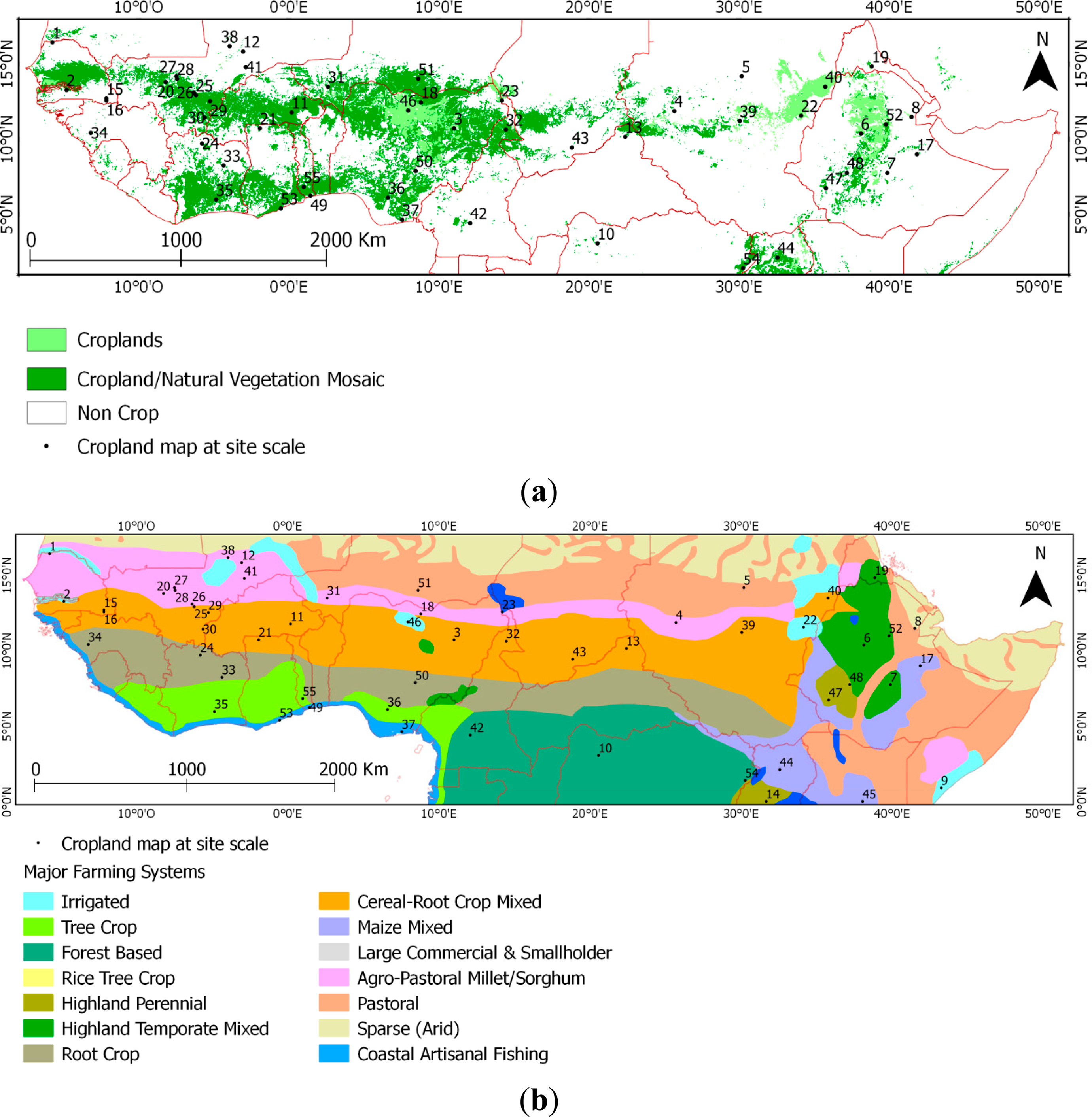
The study area spans 18°W to 50°E and 0°S to 18°N (Figure 1). It encompasses 29 countries from the Sahelian belt to the Equator. The region is characterized by a broad north–south climatic gradient that is mainly controlled by the dynamics of the Intertropical Convergence Zone. An east-west climatic contrast is also observed. Specifically, the Horn of Africa is characterized by a desert climate, whereas the West is mainly characterized by a semi-arid to tropical climate. These two climatic classifications are separated by the Ethiopian Highlands, which are characterized by a more temperate climate [35]. Over much of this region (i.e., the Sahelian, East and Horn regions), where the staple foods rely on rainfed agriculture, food shortages frequently occur in the aftermath of severe drought events.
2.2. The MODIS Land Cover Product (MCD12Q1)
The MODIS Land Cover Product (MCD12Q1, version 51, “Land Cover Type Yearly L3 Global 500 m SIN Grid”) is used to extract the cropland domain. The MODIS LCP is produced by Boston University and it provides data that characterizes five global land cover classification systems on a calendar-year basis and at a 500 m spatial resolution. The product uses data from the MODIS instrument, such as spectral and temporal information from channels 1–7, the vegetation index and land surface temperature. The MODIS land cover classification is based on a supervised approach with a multitemporal decision tree algorithm [15,16]. The MODIS land cover data were acquired for each year from 2001–2011. Two cropland classes were used (Figure 1a). The following definitions are from [37]:
The Croplands (class 12): “Land cover with temporary crops followed by harvest and bare soil period (e.g., single and multiple cropping systems. Note that perennial woody crops will be classified as the appropriate forest or shrub land cover type”.
The Cropland/Natural Vegetation Mosaic (class 14): “Land with a mosaic of croplands, forest, shrublands, and grasslands in which no one component comprises more than 60% of the landscape.”
Training data for the MCD12Q1 v51 product include 313 sites distributed across Africa, 59 of which are croplands (29 are classified as Cropland and 30 are classified as Cropland/Natural Vegetation Mosaic). The overall accuracy of the MCD12Q1 product across all classes is ∼75% [16].
2.3. Reference Datasets
The MODIS LCP cropland domain was compared with reference datasets derived from (i) agricultural statistics and (ii) a set of high-resolution image classifications.
2.3.1. Agricultural Statistics Data
FAOSTAT: This database [37] is accessible online. In this study, cropped cultivated areas and cultivated area fractions at the national scale were derived from “arable land” data. The FAO database defines arable land as “the land under temporary agricultural crops (multiple-cropped areas are counted only once), temporary meadows for mowing or pasture, land under market and kitchen gardens and land temporarily fallow (less than five years). The abandoned land resulting from shifting cultivation is not included in this category” [37].
AGRHYMET: Surface-harvested data from ground surveys of major staple crops in Burkina Faso were used. These ground surveys are conducted every year by AGRHYMET at the provincial scale (two levels below the national scale). The number of surveyed villages per province is proportional to the size of the province. Five households within each village are surveyed. Burkina Faso was chosen because it is the only country for which data at two subnational scales (regional and provincial scales) are available for 2001–2011.
2.3.2. High-Resolution Images
Based on a recent study by Tsendbazar et al. [38], which assessed global land cover reference datasets, none of the numerous datasets that currently exist were considered appropriate in our study. Specifically, these datasets inherently have the same uncertain accuracy problems as the previous global land cover maps. A specific validation dataset was therefore created. It is composed of 55 cropland maps that each covers an area of 5 × 5 km (100 MODIS pixels). The 55 sample locations were chosen to represent the study area in terms of agricultural landscapes based on the Farming Systems Maps for Sub-Saharan Africa from the FAO (Figure 1b). At least three sample locations for each farming system were used. In addition, the number of sample locations per farming system was consistent with the size of the farming system within the area. Forty-nine cropland maps were obtained by photo-interpretation of high-resolution images from GoogleEarth© and were classified as either crop or non-crop. GoogleEarth© images across Sub-Saharan Africa are mainly from Digital Globe (<10 m resolution) and were acquired between 2007 and 2013. This dataset was completed with six available crop maps that were also obtained from high-resolution images:
Four cropland maps from multispectral SPOT images at a 2.5 m resolution for 2007 in South Mali. The images were classified using an object-based supervised classification method and validated with ground data [32].
One cropland map from multispectral SPOT images at a 10 m resolution for 2010 in West Niger. A pixel-based supervised classification method was applied [39].
One cropland map from Landsat images at a 30 m resolution for 2006 in North Cameroun. The images were classified by a pixel-based supervised classification method and were also validated with ground data [40].
3. Methods
The methodology consists of first assessing the ability of the MODIS LCP to quantify crop areas by conducting comparisons with agricultural statistics datasets at various spatial scales. Then, the spatial accuracy of the MODIS LCP cropland domain was analyzed via comparisons with reference cropland maps from high-resolution images.
3.1. Assessing Quantification of Crop Areas
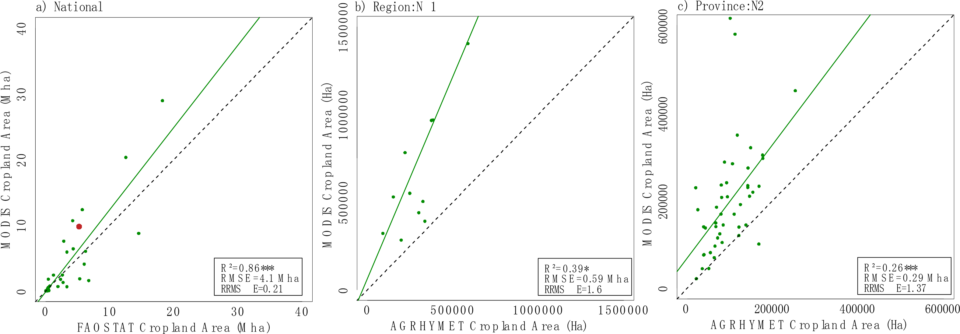
The MODIS LCP cropped areas were extracted for administrative units (at the country level for all countries and at the regional and provincial levels for Burkina Faso), and the mean between 2001 and 2011 was computed. The same procedure was also applied to the agricultural statistics data. The MODIS LCP cropped areas were compared with FAOSTAT data at regional and national scales and with AGRHYMET Burkina Faso data at regional (level 1 below national—N1) and provincial (level 2 below national—N2) levels. For areal calculations of the MODIS dataset, the numbers of pixels classified as crops were multiplied by the area of each pixel. As in Vintrou et al. [32], a weight of 0.5 was applied to the mixed class to take into account the fraction of crops according to the FAO mixed class definition [41].
Then, the crop area dynamics of the statistical and MODIS LCP data were compared at different scales. Trends in crop areas were detected using ordinary least square regression (OLS) and were found statistically significant at the 10% threshold (p-value < 0.1). The slope coefficients of the trend lines were used to determine the signs and magnitudes of the trends, i.e., a measure of the increase or decrease in the crop areas over time.
3.2. Assessing the Spatial Distribution Accuracy of Crop Areas
Conventional methods of accuracy assessments, such as the overall accuracy or per-class accuracy, are global and provide an assessment of the quality of the entire map. However, as shown by Strahler et al. [34], errors are not evenly distributed across space. For this reason, we adopted a spatially explicit assessment of map uncertainties where the MODIS LCP crop spatial distribution in 2011 was compared with the 55 reference cropland maps using the following:
- (1)
Error matrices, omission errors, commission errors and the FScore [42]. The crop class of the MODIS LCP is equal to class 12 and class 14 weighted by 0.5 (see Section 3.1).
- (2)
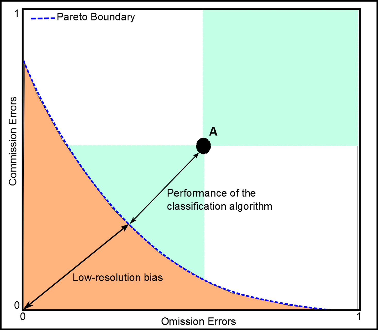
The Pareto Boundary method. The Pareto Boundary is calculated using (i) a high-resolution reference map (crop/non-crop classification) and (ii) a low-resolution pixel size. The low-resolution grid is matched to the high-resolution reference map, and the percentage of a specific class (here, the crop class) is assigned to each low-resolution pixel. We determine a set of threshold values for the percentage of the crop class that is present within the low-resolution pixels; values above these thresholds are classified as crops. For each threshold, omission and commission errors are computed. Finally, a line joining this set of omission and commission error pairs is drawn to represent the Pareto Boundary (for more details, see [43]). In addition, by counting the number of reference pixels for a specific class (here, the crop class) within the global product pixels, the Pareto Boundary permits an analysis of the influence of the low spatial resolution on the accuracy of the final thematic product. The Pareto Boundary also presents the concept of the “optimal” accuracy (the point minimizing the user-producer errors) that could theoretically be attained and delimit a region of unattainable accuracy due to the low-resolution bias (Figure 2). In this study, the “optimal” accuracy was estimated for the MODIS LCP and the other sensors by simulating grids at 300 m, 30 m and 10 m spatial resolutions to assess the accuracy that could be attained given the sensor used. The distance between the “optimal” accuracy derived from the Pareto Boundary and the accuracy derived from a given thematic map represents an index of the performance of the classification algorithm. An advantage of the Pareto Boundary method is that aggregation of the fine-resolution reference map to the coarse resolution of the global product is not required [2].
3.3. Characterizing Landscape Patterns
- (1)
Landscape fragmentation. The Pareto Boundary and, consequently, the map accuracy can be linked with landscape fragmentation. Landscape fragmentation is mainly caused by the spatial heterogeneity in biophysical conditions and the history of land occupation [44]. As stated previously by Mayaux and Lambin [45], the statistical distribution of patch sizes and shapes and their spatial distribution and connectivity are elements that are used to characterize landscape structures. Each spatial pattern can be described with several indicators. In this study, we used the Crop Fraction, the Matheron Index [45], the Compactness Index [46], the Mean Focal Diversity [20], the Crop Patch Density and the Crop Edge Density [47] to express the agricultural landscape fragmentation (Table 1). Each index was calculated based on the MODIS LCP product for 2011 and within a grid size of 5 km.
- (2)
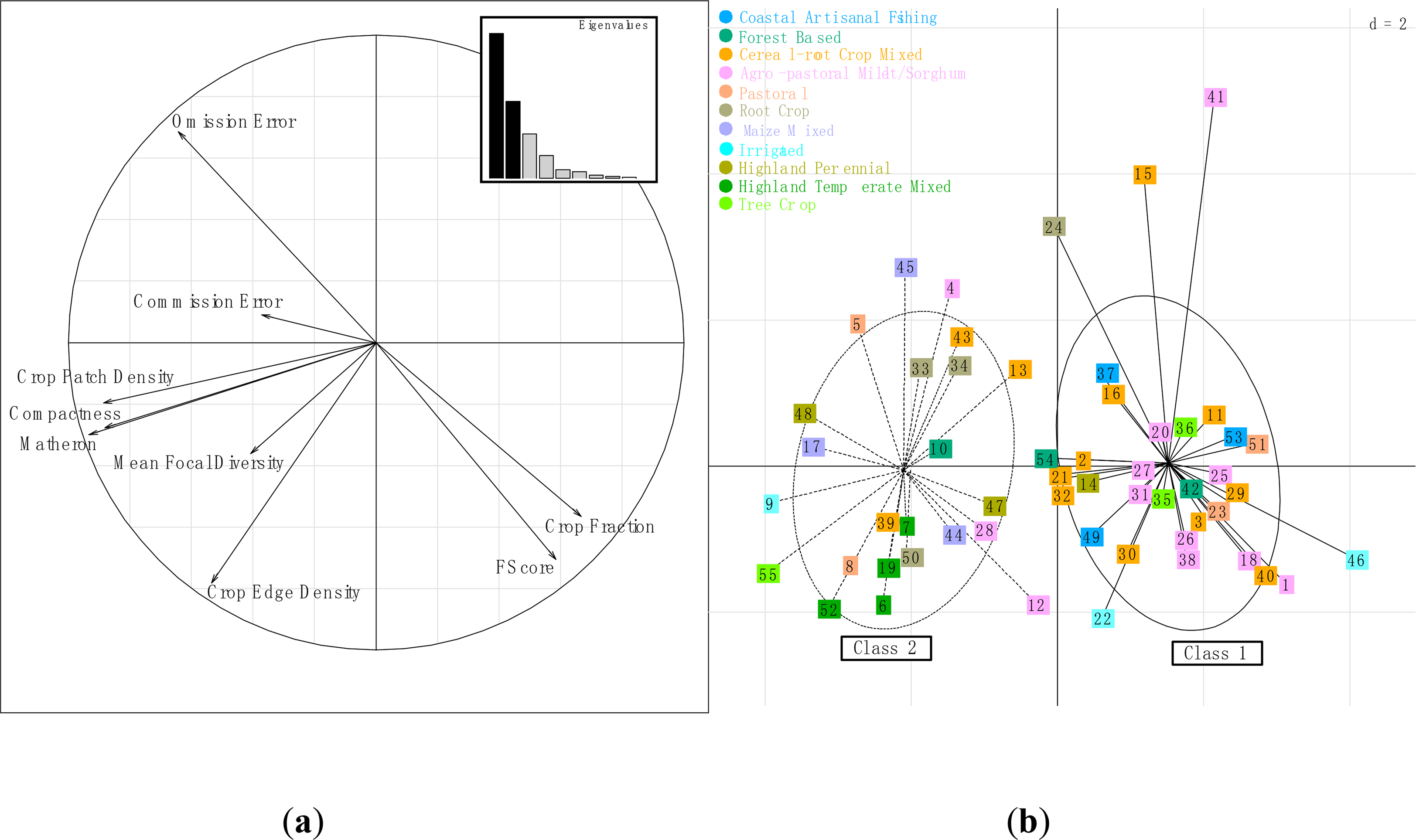
Analysis of the landscape metric. A normalized PCA (principal component analysis) was computed using the ADE-4 package [48] within R software. PCA reduces the size of the dataset and statistically verifies links between the three spatial accuracy indicators (omission, commission and Fscore) and the six fragmentation indices. Thus, PCA permits an analysis of the similarities between the 55 sites. In addition, according to their landscape fragmentation and farming system similarities, the sites were partitioned into homogeneous classes by K-Means clustering. Then, multiple linear regression was applied to the accuracy indicators (dependent variables) and the six fragmentation indicators (explanatory variables). A multiple linear regression model was fitted at the reference dataset scale. The model selection was conducted using the Bayesian Information Criterion (BIC) [49].
4. Results
4.1. Comparison of the MODIS LCP and the Statistical Crop Area Data
4.1.1. Comparison of the Crop Areas at Different Spatial Scales
At sub-Saharan Africa scale, estimates of the total crop areas by the MODIS LCP are found to be close to those of FAO (13% of the total area for MODIS and 11% for FAO). At national scale, the MODIS LCP provide close estimates, with R2 equal to 0.86 (pvalue < 0.001), RRMSE equal to 0.21 and a slight over-estimation compared to FAO estimates (Figure 3a). This is unlike in Fritz et al. [1] where MODIS provided lower estimates than FAO statistics for 10 countries of our study area. The difference may be partly explained by the use of a previous version of the MODIS LCP (MCD12Q1 v4) in [1]. However, at the N1 or N2 levels in Burkina Faso (Figure 3b,c, respectively), the comparison shows high discrepancies between the crop area estimates. In both cases, R2 is below 40%, with a clear over-estimation by the MODIS LCP. This is in agreement with Hannerz and Lotsch [11], who found an inverse relationship between MODIS and AGRHYMET data for Burkina Faso.
4.1.2. Comparison of Cropland Area Dynamics
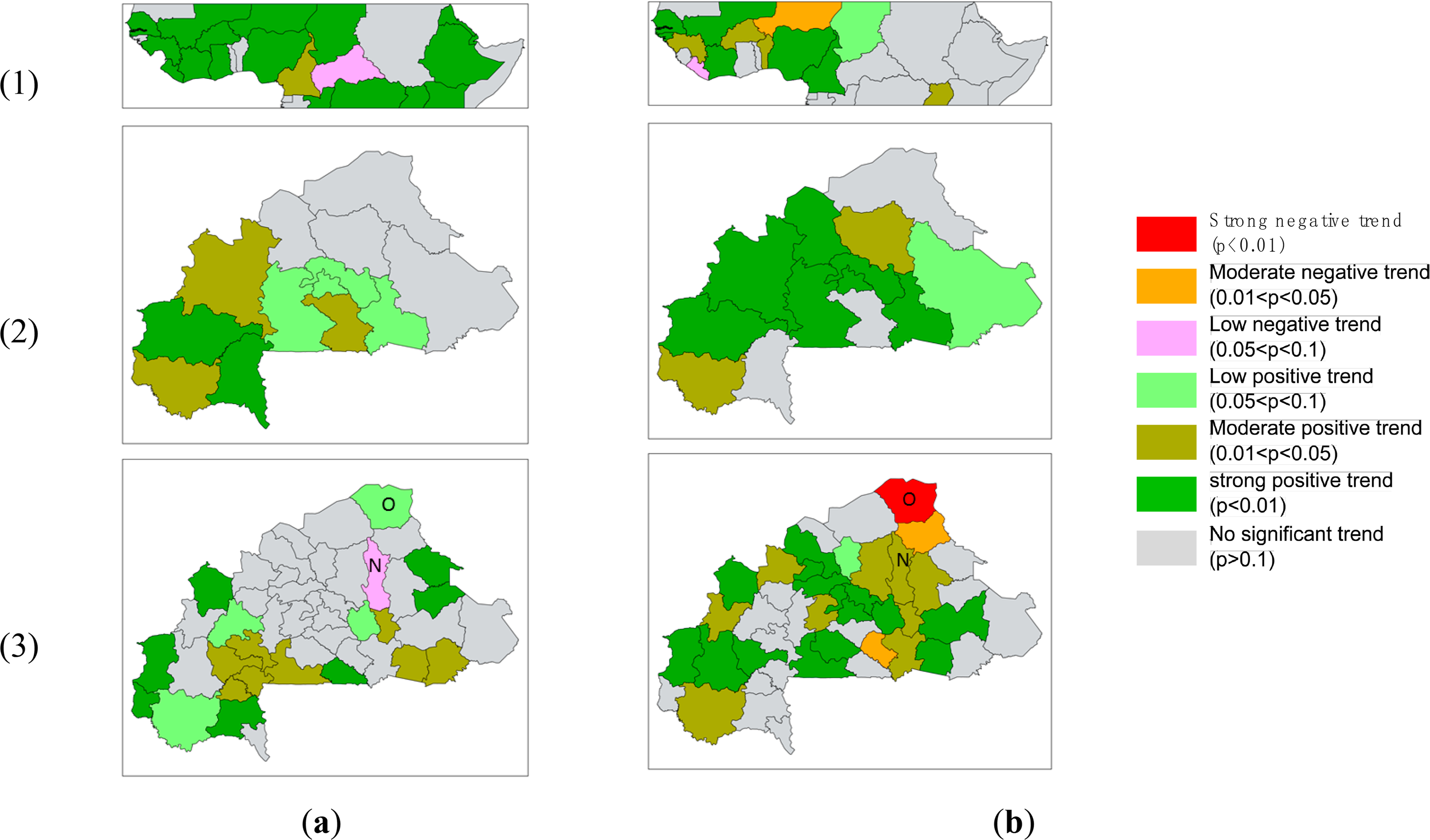
A comparison between the MODIS LCP and statistical dynamics reveals discrepancies, depending on the scale considered (Figure 4). At the national scale, the same positive trend (overall increase in cropland area) can be observed in West Africa with, however, opposite dynamics for Liberia and Niger Figure 4 1a,1b). In East Africa, FAO shows a positive trend, whereas no significant trends are detected in the MODIS LCP. This can partly be explained by the fact that in this part of Africa, many agricultural systems are based on agroforestry or pastoralism and are therefore not included in the crop classes of the MODIS LCP. At the N1 scale in Burkina Faso, both the MODIS LCP and AGRHYMET data show positive dynamics of crop areas in the West but differences in the eastern part of the country. There, no significant dynamics are found with AGRHYMET, whereas the MODIS LCP shows positive dynamics (Figures 2a,b and 4). A similar situation is observed at the N2 scale but with higher discrepancies between the two datasets and opposite dynamics for the provinces of Oudalan and Namentenga (Figures 3a,b and 4).
4.2. Spatial Accuracy of Crop Area Distribution: MODIS LCP vs. High-Resolution Classifications
Error matrices between the MODIS LCP and high-resolution classifications were calculated for the 55 validation sites (Table 2). There is considerable variability in the accuracy of the MODIS LCP across the different sites. The average omission error for all sites is equal to 0.56, the average commission error is equal to 0.46, and 35 out of the 55 sites have an FScore lower than 0.50; thus, overall, the MODIS LCP exhibits a moderate accuracy in the crop area distribution.
The best accuracy was observed for site 46 (0.03 omission error, 0.13 commission error and an FScore equal to 0.92), whereas the lowest accuracy was obtained for site 5 (0.90 omission error, 0.99 commission error and an FScore equal to 0.01). The Pareto Boundary was also used and allowed to estimate the “optimal” accuracy that could be attained with the MODIS LCP. The Pareto Boundary enabled the computation of the observed/optimal distance as the Euclidean distance between the observed and “optimal” accuracies. This distance is an indicator of the MODIS LCP classification algorithm performance. As shown in Table 2, most of the sites have an observed/optimal distance larger than 0.50, indicating a moderate to poor performance of the MODIS LCP classification algorithm.
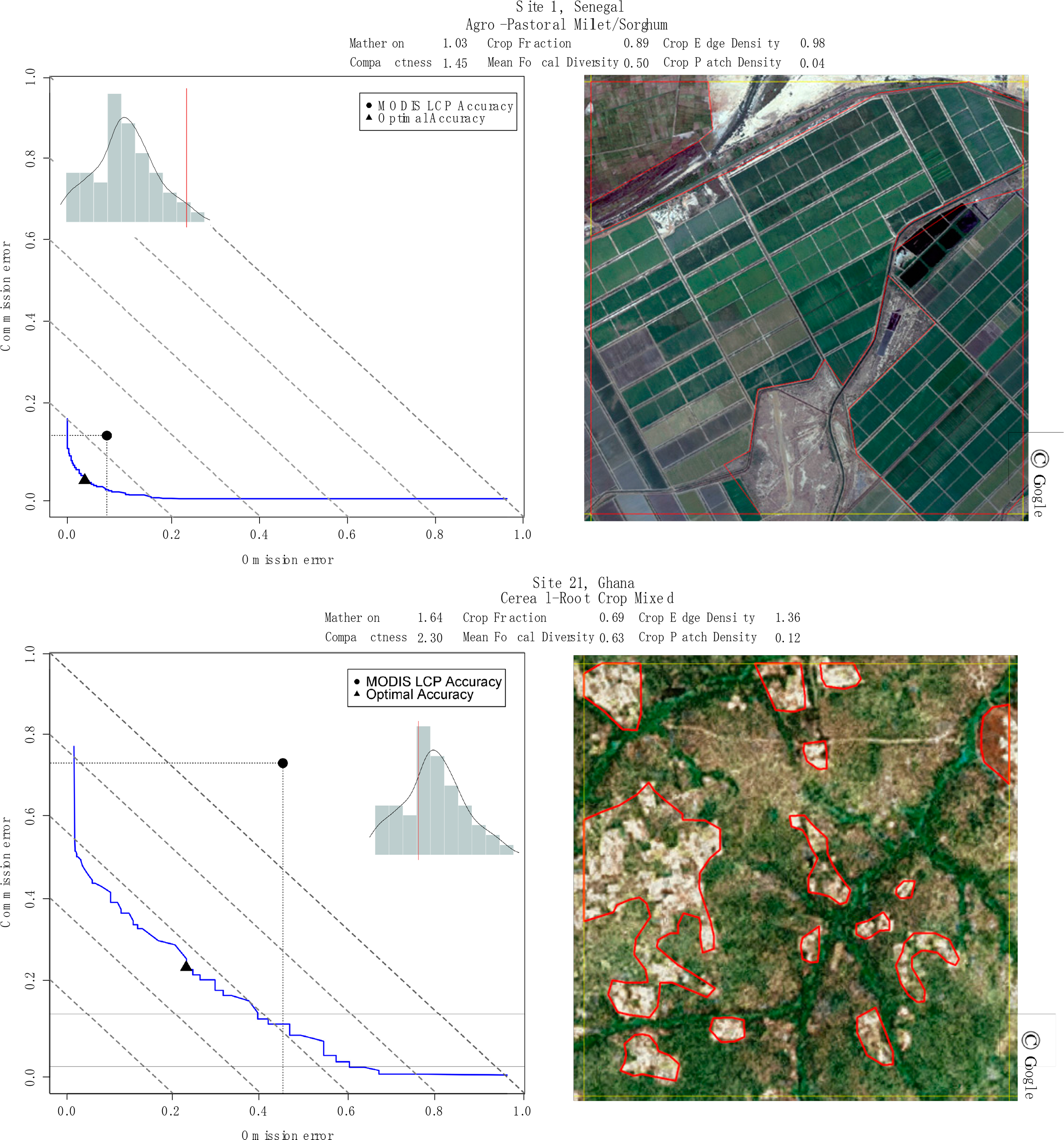
Figure 5 presents two examples of Pareto Boundaries. The previous commission and omission errors are used to obtain the Pareto Boundary. The Pareto Boundary is higher for the sites that are most fragmented and heterogeneous (site 21); it is between the 50% and 80% isoline. For the most homogeneous site (site 1), the Pareto Boundary is the lowest and close to the 10% isoline. Overall, the accuracy of the MODIS LCP is lower when fragmentation is high (high uncertainty in the localization of the cropland classes). The PCA summarizes our findings for all of the validation sites and provides links between the accuracy and fragmentation indicators (Figure 6a,b). In addition, it was possible to analyze the site similarities according to their farming system and landscape fragmentation using K-Means clustering (Figure 6b). The first two components of the PCA used for the accuracy and fragmentation indicators explain 71% of the total variance (Figure 6a). The first PCA axis tends to align Coastal Artisanal Fishing, Agro-Pastoral Millet/Sorghum and Cereal-Root Crop Mixed farming systems (class 1) against Highland Perennial, Maize Mixed, Highland Temperate Mixed and Root Crop farming systems (class 2) (Figure 6b). The other farming systems have a less clear pattern. Coastal Artisanal Fishing, Agro-Pastoral Millet/Sorghum and Cereal-Root Crop Mixed farming systems (class 1) are associated with a high crop fraction and a high FScore (Figure 6a,b). In contrast, Highland Perennial, Maize Mixed, Highland Temperate Mixed and Root Crop farming systems (class 2) are characterized by high omission errors. The PCA analysis also suggests that commission errors and landscape fragmentation are not correlated.
4.3. Spatial Heterogeneity and Fragmentation vs. Mapping Uncertainties
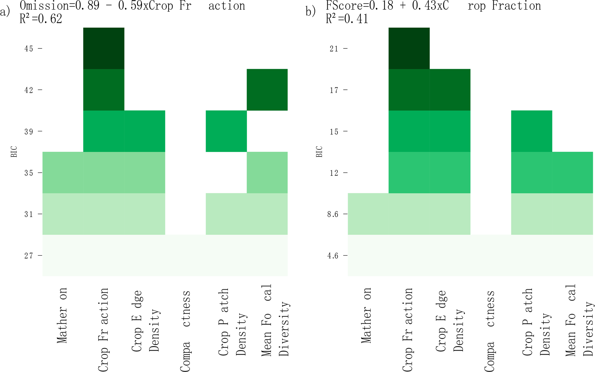
The previous section showed that agricultural landscape fragmentation and spatial heterogeneity affect the accuracy, particularly the omission errors and FScores, of the MODIS LCP for crop areas. Figure 7 presents the results of multiple linear regressions computed for validation sites between the six indicators of landscape metric fragmentation (explanatory variables) and the accuracy indicators.
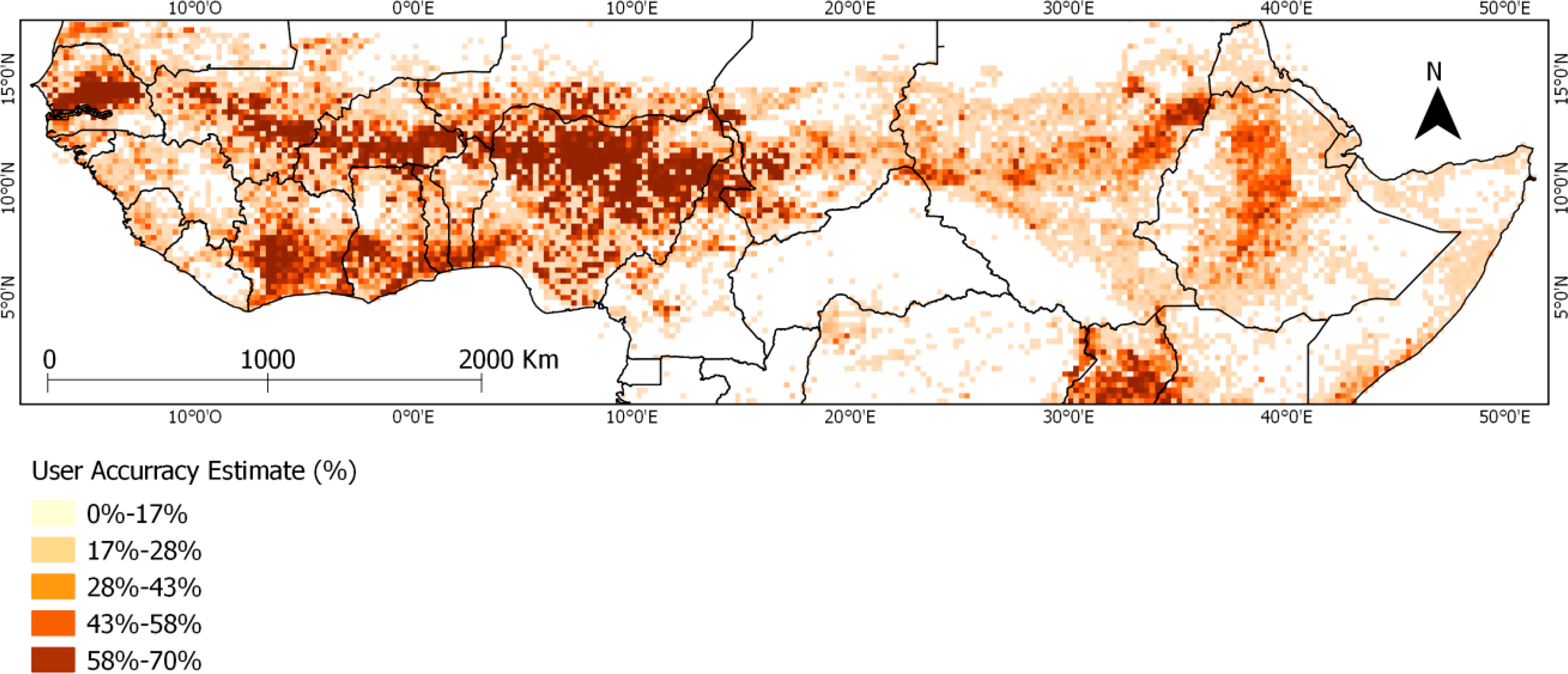
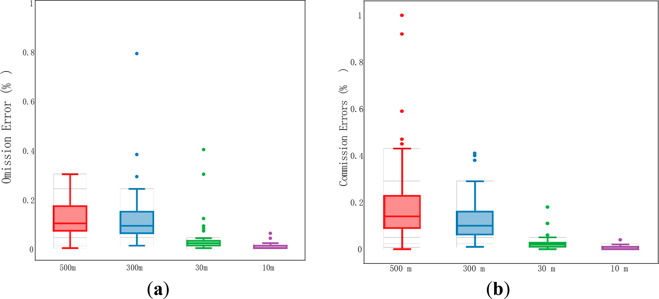
Figure 7a shows a strong relationship between the omission errors and the Crop Fraction in which 62% of the omission error variability of the MODIS LCP is explained by the Crop Fraction. The relationships between the landscape metric fragmentation and the FScore are less clear (R2 = 0.41; Figure 7b). To illustrate how the MODIS LCP accuracy is spatially distributed, a map of user accuracy estimates for cropland classes was produced by applying the linear regression model previously developed by the BIC to the entire MODIS LCP dataset (Figure 8). The maximum user accuracy that could be attained given the agricultural landscape patterns is ∼70%, with an omission error of at least 30%. However, most pixels have a user accuracy of 0%–28%, indicating a high degree of uncertainty in the localization of the cropland domain. The user accuracy is better in the West than in the East and is mainly related to Agro-Pastoral Millet/Sorghum and Cereal-Root Crop Mixed farming systems (see Figure 1 and Table 3). Finally, an assessment of the “optimal” accuracy that could be attained with higher spatial resolution datasets (300 m, 30 m and 10 m) was performed (Figure 9). Regarding the omission and commission errors, an improvement of the accuracy values was observed; the accuracy variability decreased between sites. The relative standard deviations of the omissions and commissions were equal to 7% and 19% at 500 m, respectively, 11% and 9% at 300 m, respectively, 6% and 3% at 30 m, respectively, and less than 1% at 10 m. Thus, the use of a sensor with a higher spatial resolution, such as the future Sentinel-2 system, may lead to improved accuracy and spatial homogeneity of cropland maps.
5. Discussion
Assessing the quality and the reliability of Global Land Cover Products, such as the MODIS LCP, in both the localization and the estimation of crop areas in the fragmented agricultural landscape of Sub-Saharan Africa is essential for appropriately using these products. An original approach based on agricultural statistical databases and cultivated maps derived from high-resolution classifications were used in this study to assess the suitability of the MODIS LCP for crop area mapping.
5.1. Comparison of the MODIS LCP and Statistical Data
Regarding crop areal estimations and their dynamics, the results show that the correlation between statistical data and the MODIS LCP decreases when the spatial scale is localized. The differences observed at the national scale could be due to fallows. FAOSTAT data include fallows of less than five years, whereas such information is not given in the MODIS product. Thus, it is likely that older fallows were included in our estimates. Moreover, because of uncertainties in their accuracy, timelessness, and consistency over time across countries and crop types, official national FAO statistics are certainly subject to errors that can limit their ability to quantify the spatial extent of crop areas [7,9,11,50]. However, as mentioned recently by Vancutsem et al. [28], this dataset remains a helpful source of information for assessing the quality of Global Land Cover products, such as the MODIS LCP. At subnational scales, the differences could partly be explained by the fact that some discrepancies in crop areal estimations at fine spatial scales (e.g., the province level) are masked when aggregating to coarser scales. This has already been highlighted by Hannerz and Lotsch [11] for statistical data and by Mayaux and Lambin [45] in a study where they analyzed the effects of spatial aggregation of remote sensing data on the estimation of tropical forest areas; these studies concluded that information was lost in the process of scaling up. Another reason for these differences may be that AGRHYMET does not include fallows in their statistics, while fallows are most likely included in the MODIS LCP estimates. As mentioned previously by Wu et al. [5], fallow areas are often not reported in cropland products due to their temporal dynamics and confusion with other land cover types.
5.2. Spatial Accuracy of the MODIS LCP
At the global scale, human activities, such as agricultural practices, have shaped the landscape and landscape fragmentation and heterogeneity correspond to a higher unreachable region of the Pareto Boundary and a lower accuracy. At the global scale, Herold et al. [20] found an omission error equal to 7.9% (user accuracy equal to 92.1%) and a commission error equal to 35.2% (producer accuracy equal to 64.8%) for the crop classes. These results are, on average, different from our results (our omission error is equal to 56% and our commission error is equal to 42%, on average) and can be explained by three main factors: (1) the study was conducted at the global scale and included large homogeneous agricultural landscapes, such as the Great Plains, USA, whereas the agricultural landscapes of Sub-Saharan Africa are known to be highly fragmented; (2) the MODIS LCP used in [20] was a different version, with a 1 km resolution, and was less spatially accurate than the version in the present study; and (3) the 0.5 weight was not applied to class14. Yet, our results are not too different from those of Friedl et al. [16] and Ran et al. [27]; the former also used the MODIS LCP v5 at the global scale. Together, class12 and class14 (0.5 weight) produced an omission error of 46.7% and a commission error of 43.3% based on the training sites. Ran et al. found an overall accuracy of 65.09% for the cropland class (our overall accuracy is 51%, on average). Following the cropland class definition given in [40], we assumed that the crop proportion was fixed, and we applied a 0.5 weight to class14 and no weight to class12. However, in reality, the proportion may vary between ∼0% and 50% for class14 and between 60% and 100% for class12. Consequently, we can assume that the accuracy obtained here may evolve, depending on the weight applied.
5.3. Relationship between Spatial Accuracy, Landscape Fragmentation and Farming Systems
Agricultural landscapes of smallholder farms, such as those in Sub-Saharan Africa, are characterized by small parcels (typically ≤ 2 ha) [51]. Consequently, in areas with low cropping intensities, high omission errors could be due to the inability of the MODIS LCP to capture crop patches that are often smaller than a pixel size (∼25 ha). Furthermore, important commission errors could be a result of the large pixel size where non-crop areas that surround crop areas (mainly grassland or shrubland) could be mapped as cropland areas, as explained by Wardlow and Egbert [52] and recently by Vintrou et al. [32]. In addition, some studies have also highlighted the difficulties in mapping cultivated areas, mainly in the Sahel, due to the high degree of ambiguity of assigning a single class to a heterogeneous landscape composed of natural vegetation and croplands, which have spectral, textural and temporal similarities [10,11,23]. Consequently, the Cropland/Natural vegetation mosaic class of the MODIS LCP may group different classes together. This can have a significant impact on the final accuracy [2] and lead to an over- or under-estimation of crop areas [4,21].
The PCA clearly showed that spatial heterogeneity and fragmentation is a major driver of the accuracy, particularly the user accuracy, of the MODIS LCP in Sub-Saharan Africa. Our results are in agreement with prior studies of various regions of the world that show a strong relationship between landscape fragmentation and map accuracy at low spatial resolutions; specifically, the accuracy decreases as fragmentation and heterogeneity increases [26,30,42,53]. For example, in the study of Gao and Jia [24] on the tolerance of misclassification within the MODIS LCP in China, the authors found that misclassifications are higher in heterogeneous landscapes of southern China that are characterized by highly diverse and fragmented vegetation types. Although our results corroborate prior studies, the present work also provided a quantification of the intuitive relationship between landscape fragmentation and classification accuracy to establish a map of user accuracy estimates for cropland classes. The results showed that the user accuracy is lower for the eastern part of the study area, which mainly consists of Maize Mixed, Highland Perennial and Highland Temperate Mixed farming systems (class 2; Table 3). This finding can be explained by (1) the very small farm sizes compared to other farming systems, in which more than 50% of the farms are smaller than 0.5 ha in Highland Perennial farming systems or in Maize Mixed farming systems [54] and (2) the Highland Temperate Mixed farming systems located at altitudes higher than 1800 m are associated with small farm sizes (∼1.6 ha) [54] and greater fragmentation of the landscape due to slopes [54]. These results suggest that, to enhance the MODIS LCP crop area mapping, a primary challenge is to improve the mapping of heterogeneous landscapes.
5.4. “Optimal” Accuracy of Land Cover Products
When assessing the accuracy of a coarse-resolution map, the resolution of the high-resolution validation dataset is often aggregated to match the resolution of the coarse-resolution map, and the dominant class is assigned to the new pixel [2,55]. The use of the Pareto Boundary allowed us to compare the MODIS LCP with high-resolution data without degrading the fine resolution of our validation datasets. This is a useful tool for estimating the “optimal” user and producer accuracies that could be attained by the MODIS LCP given the low-resolution bias and fragmentation. However, the Pareto Boundary is not based on the actual low-resolution map but rather on the low-resolution grid; consequently, uncertainty in the positioning of the low-resolution grid may affect the omission and commission errors. In a very highly fragmented area of Central Africa, Boschetti et al. [43] found that the uncertainty in the positioning of the low-resolution grid had a negligible effect on the positioning of the Pareto Boundary. Thus, misregistration effects on the Pareto Boundary were also neglected in our study. The MODIS LCP “optimal” accuracy at most of the sites is above 50%, which indicates a high degree of uncertainty. The majority of the sites in the Irrigated, Agro-Pastoral Millet/Sorghum and Cereal-Root Crop Mixed farming system zones tend to have minimal omission-commission errors. Therefore, for agricultural statistics, we suggest that areal estimates of other farming systems be used with caution. Moreover, regardless of the resolution, the performance of the classification algorithm can be identified by analyzing the distance between the “optimal” accuracy and the actual accuracy using the Pareto Boundary. For most of our sites, the classification algorithm performed poorly, i.e., the observed/optimal Euclidean distance was larger than 0.50. This may be due to the validation procedure of the MODIS LCP, as it is not based on statistically robust sampling and local experts do not perform the validation [1,20,21]. Finally, the “optimal” accuracy computed for the simulated data with a higher spatial resolution permitted us to evaluate the expected accuracies for other datasets in the case of a perfect algorithm. This highlights the need to strengthen initiatives for the creation of finer resolution land cover maps, such as the Chinese project that intends to map the global land cover based on Landsat imagery [56].
5.5. Validation Databases
Given the lack of datasets at high spatial resolutions in Africa to validate Global Land Cover Products, the use of GoogleEarth© data as a reference dataset proved valuable in assessing the quality and accuracy of the MODIS LCP. Photo-interpretation of high-resolution images is more time-consuming than automatic classifications but much less time-consuming than ground surveys. Consequently, the approach represents a good trade-off for accuracy assessments. GoogleEarth© was already used for the validation of the GlobCover product [17] and in the recent study of Vancutsem et al. [27]. In this study, 55 validation sites were used to assess the quality of the MODIS LCP, and given the extent of the area considered, we are aware that this is a small sample. However, we are foremost presenting a methodological approach, which should be reinforced with more validation sites. In this sense, new initiatives such as the Geo-Wiki project [32] or the ESA GOFC-OLD project [1] could be used. These projects aim to provide global validation databases for accuracy assessments of Global Land Cover Products through a web portal.
5.6. Practical Recommendations
Because two different maps may have the same overall accuracy but different spatial qualities, the need for assessing the spatial distribution of accuracy was highlighted in this paper. Based on our results, we provide some recommendations for practical applications of Global Land Cover Products. We suggest the use of high-resolution data to identify the relevance of a global product. For example, for early warnings, timely and objective information on crops is needed. In this particular context, especially when yields are modeled spatially, greater importance must be given to the user accuracy (or omission errors) because it signifies the probability that a pixel classified as crops represents crops on the ground and thus mitigates over-estimations of yields. Likewise, for crop acreage estimations, we recommend emphasizing the importance of user accuracy to avoid over-estimating crop areas. Conversely, in situ where information on land cover changes is required (such as in agricultural planning and decision support), we advise giving the same weight to both omission and commission errors. Thus, the key idea of this study is that it is necessary to estimate the accuracy of land cover products, anticipate product limitations and ensure an appropriate usage that corresponds to the user needs.
6. Conclusions
In this paper, we analyzed the reliability and ability of the MODIS Land Cover Product (LCP) to map crop areas in Sub-Saharan Africa.
First, we compared the MODIS LCP and agricultural statistics to estimate the accuracy of the MODIS LCP for crop area estimations. We found the ability of the MODIS LCP to estimate crop areas and its dynamics to be satisfactory at regional and national scales (R2 = 0.86 ***), but precautions must be taken for crop acreage estimations at finer scales.
Then, we assessed the spatial distribution accuracy of the MODIS LCP. Specifically, a high-resolution dataset was employed, and the confusion matrix and Pareto Boundary methods were applied. We found a strong relationship between the user accuracy and the fragmentation of the agricultural landscape with a R2 equal to 0.62 ***. Based on this finding, we produced a map of user accuracy estimates over the region. We found that the MODIS LCP user accuracy was superior for three farming systems: Agro-Pastoral Millet/Sorghum, Cereal-Root Crop Mixed and Irrigated farming systems. To our knowledge, this is the first attempt to map global land cover uncertainties for a specific class at such a scale. Because of the moderate resolution, the MODIS LCP has an inherent limitation in discriminating low cropping pixels due to the subpixel heterogeneity [11,29]. However, it represents a valuable approach for determining cropland areas from a consistent land cover map at a large scale.
Overall, mapping crop areas in fragmented landscapes from coarse-resolution data remains a difficult task and a significant challenge. However, initiatives such as the GEO-Global Agricultural Monitoring Project (GEO-GLAM Project) have started to work at improving global agriculture monitoring and crop production estimations [57]. In addition, the forthcoming Sentinel-2 satellites will routinely deliver high-resolution images (10 m resolution) and are expected to significantly contribute to the current efforts. With their high temporal resolution, agricultural land cover maps and information on agricultural land use practices (crop type, cropping intensities, irrigation, and crop rotation) could be provided regularly. However, for present and future agricultural monitoring, historical datasets will continue to be important for understanding the processes that shaped the agricultural landscapes. Thus, it is necessary to continue developing methods for handling past data.
Acknowledgments
This study was funded by Louise Leroux’s CIRAD fellowship and by the Centre National d’Etudes Spatiales (Project CNES-TOSCA “Dynafrique”). The authors thank the MODIS team for sharing the MODIS Land Cover Product and Elodie Vintrou and Kadidiatou Yéro Souley for providing the crop masks in Mali and Niger, respectively. Finally, the authors thank the AGRHYMET Center in Niamey for providing the agricultural statistics in Burkina Faso.
Author Contributions
Agnès Bégué and Danny Lo Seen developed and supervised the research. Louise Leroux is the principal author of this paper and processed and analyzed the majority of the data. Audrey Jolivot performed the photo-interpretation of the high-resolution images and computed the fragmentation metrics. Bernardin Zoungrana provided the AGHRYMET statistical data and contributed to the preprocessing and analysis of the dataset.
Conflicts of Interest
The authors declare no conflict of interest.
References
- Olofsson, P.; Stehman, S.V.; Woodcock, C.E.; Sulla-Menashe, D.; Sibley, A.M.; Newell, J.D.; Friedl, M.; Herold, M. A global land-cover validation data set, part I: Fundamental design principles. Int. J. Remote Sens 2012, 33, 5768–5788. [Google Scholar]
- Pflugmacher, D.; Krankina, O.N.; Cohen, W.B.; Friedl, M.; Sulla-Menashe, D.; Kennedy, R.E.; Nelson, P.; Loboda, T.V.; Kuemmerle, T.; Dyukarev, E.; et al. Comparison and assessment of coarse resolution land cover maps for Northern Eurasia. Remote Sens. Environ 2011, 115, 3539–3553. [Google Scholar]
- Fritz, S.; See, L. Identifying and quantifying uncertainty and spatial disagreement in the comparison of Global Land Cover for different applications. Glob. Chang. Biol 2008, 14, 1057–1075. [Google Scholar]
- Giri, C.; Pengra, B.; Long, J.; Loveland, T. Next generation of global land cover characterization, mapping, and monitoring. Int. J. Appl. Earth Obs. Geoinf 2013, 25, 30–37. [Google Scholar]
- Wu, Z.; Thenkabail, P.S.; Mueller, R.; Zakzeski, A.; Melton, F.; Johnson, L.; Rosevelt, C.; Dwyer, J.; Jones, J.; Verdin, J.P. Seasonal cultivated and fallow cropland mapping using MODIS-based automated cropland classification algorithm. J. Appl. Remote Sens 2014, 8, 18. [Google Scholar]
- Husak, G.J.; Marshall, M.T.; Michaelsen, J.; Pedreros, D.; Funk, C.; Galu, G. Crop area estimation using high and medium resolution satellite imagery in areas with complex topography. J. Geophys. Res 2008, 113, D14112. [Google Scholar]
- Fritz, S.; See, L.; Rembold, F. Comparison of global and regional land cover maps with statistical information for the agricultural domain in Africa. Int. J. Remote Sens 2010, 31, 2237–2256. [Google Scholar]
- Wu, W.; Shibasaki, R.; Yang, P.; Zhou, Q.; Tang, H. Remotely sensed estimation of cropland in China: A comparison of the maps derived from four global land cover datasets. Can. J. Remote Sens 2008, 34, 467–479. [Google Scholar]
- Justice, C.; Becker-Reshef, I. Developing a Strategy for Global Agricultural Monitoring in the Framework of Group on Earth Observations (GEO) Workshop Report; Group on Earth Observations: Rome, Italy, 2007; p. 67. [Google Scholar]
- Delrue, J.; Bydekerke, L.; Eerens, H.; Giliams, S.; Piccard, I.; Swinnen, E. Crop mapping in countries with small-scale farming: A case study for West Shewa, Ethiopia. Int. J. Remote Sens 2013, 34, 2566–2582. [Google Scholar]
- Hannerz, F.; Lotsch, A. Assessment of Land Use and Cropland Inventories for Africa; Centre for Environmental Economics and Policy in Africa, University of Pretoria: Pretoria, South Africa, 2006. [Google Scholar]
- Vancutsem, C.; Pekel, J.-F.; Kayitakire, F. Dynamic mapping of cropland areas in Sub-Saharan Africa using MODIS time series. Proceedings of 2011 International Workshop on the Analysis of Multi-temporal Remote Sensing Images (Multi-Temp), Trento, Italy, 12–14 July 2011; pp. 25–28.
- Loveland, T.; Belward, A. The IGBP-DIS global 1 km land cover data set, DISCover: First results. Int. J. Remote Sens 1997, 18, 3291–3295. [Google Scholar]
- Bartholomé, E.; Belward, A. GLC2000: A new approach to global land cover mapping from Earth observation data. Int. J. Remote Sens 2005, 26, 1959–1977. [Google Scholar]
- Friedl, M.; McIver, D.; Hodges, J.C.; Zhang, X.; Muchoney, D.; Strahler, A.H.; Woodcock, C.E.; Gopal, S.; Schneider, A.; Cooper, A.; et al. Global land cover mapping from MODIS: Algorithms and early results. Remote Sens. Environ 2002, 83, 287–302. [Google Scholar]
- Friedl, M.; Sulla-Menashe, D.; Tan, B.; Schneider, A.; Ramankutty, N.; Sibley, A.; Huang, X. MODIS Collection 5 global land cover: Algorithm refinements and characterization of new datasets. Remote Sens. Environ 2010, 114, 168–182. [Google Scholar]
- Bicheron, P.; Defourny, P.; Brockmann, C.; Schouter, L.; Vancutsem, C.; Huc, M.; Bontemps, S.; Leroy, M.; Achard, F.; Herold, M.; et al. GLOBCOVER Products Report Description and Validation Report; MEDIAS: Toulouse, France, 2008. [Google Scholar]
- Kaptué Tchuenté, A.T.; Roujean, J.-L.; Faroux, S. ECOCLIMAP-II: An ecosystem classification and land surface parameters database of Western Africa at 1 km resolution for the African Monsoon Multidisciplinary Analysis (AMMA) project. Remote Sens. Environ 2010, 114, 961–976. [Google Scholar]
- Latham, J.; Cumani, R.; Rosati, L.; Bloise, M. Global Land Cover SHARE (GLC-SHARE); FAO: Rome, Italy, 2014; p. 40. [Google Scholar]
- Herold, M.; Mayaux, P.; Woodcock, C.E.; Baccini, A.; Schmullius, C. Some challenges in global land cover mapping: An assessment of agreement and accuracy in existing 1 km datasets. Remote Sens. Environ 2008, 112, 2538–2556. [Google Scholar]
- Giri, C.; Zhu, Z.; Reed, B. A comparative analysis of the Global Land Cover 2000 and MODIS land cover data sets. Remote Sens. Environ 2005, 94, 123–132. [Google Scholar]
- Kaptué Tchuenté, A.T.; Roujean, J.-L.; de Jong, S.M. Comparison and relative quality assessment of the GLC2000, GLOBCOVER, MODIS and ECOCLIMAP land cover data sets at the African continental scale. Int. J. Appl. Earth Obs. Geoinf 2011, 13, 207–219. [Google Scholar]
- McCallum, I.; Obersteiner, M.; Nilsson, S.; Shvidenko, A. A spatial comparison of four satellite derived 1 km global land cover datasets. Int. J. Appl. Earth Obs. Geoinf 2006, 8, 246–255. [Google Scholar]
- Gao, H.; Jia, G. Assessing disagreement and tolerance of misclassification of satellite-derived land cover products used in WRF model applications. Adv. Atmos. Sci 2013, 30, 125–141. [Google Scholar]
- Neumann, K.; Herold, M.; Hartley, A.; Schmullius, C. Comparative assessment of CORINE2000 and GLC2000: Spatial analysis of land cover data for Europe. Int. J. Appl. Earth Obs. Geoinf 2007, 9, 425–437. [Google Scholar]
- Pérez-Hoyos, A.; García-Haro, F.J.; San-Miguel-Ayanz, J. Conventional and fuzzy comparisons of large scale land cover products: Application to CORINE, GLC2000, MODIS and GlobCover in Europe. ISPRS J. Photogramm. Remote Sens 2012, 74, 185–201. [Google Scholar]
- Ran, Y.; Li, X.; Lu, L. Evaluation of four remote sensing based land cover products over China. Int. J. Remote Sens 2010, 31, 391–401. [Google Scholar]
- Vancutsem, C.; Marinho, E.; Kayitakire, F.; See, L.; Fritz, S. Harmonizing and combining existing land cover/land use datasets for cropland area monitoring at the African continental scale. Remote Sens 2013, 5, 19–41. [Google Scholar]
- Gonsamo, A.; Chen, J.M. Evaluation of the GLC2000 and NALC2005 land cover products for LAI retrieval over Canada. Can. J. Remote Sens 2011, 37, 302–313. [Google Scholar]
- Latifovic, R.; Olthof, I. Accuracy assessment using sub-pixel fractional error matrices of global land cover products derived from satellite data. Remote Sens. Environ 2004, 90, 153–165. [Google Scholar]
- Cohen, W.B.; Maiersperger, T.K.; Turner, D.P.; Ritts, W.D.; Pflugmacher, D.; Kennedy, R.E.; Kirschbaum, A.; Running, S.W.; Costa, M.; Gower, S.T. MODIS land cover and LAI collection 4 product quality across nine sites in the western hemisphere. IEEE Trans. Geosci. Remote Sens 2006, 44, 1843–1857. [Google Scholar]
- Vintrou, E.; Desbrosse, A.; Bégué, A.; Traoré, S.; Baron, C.; Lo Seen, D. Crop area mapping in West Africa using landscape stratification of MODIS time series and comparison with existing global land products. Int. J. Appl. Earth Obs. Geoinf 2012, 14, 83–93. [Google Scholar]
- Fritz, S.; Mccallum, I.; Schill, C.; Perger, C.; Grillmayer, R.; Achard, F.; Kraxner, F.; Obersteiner, M. Geo-Wiki.Org: The Use of crowdsourcing to improve global land cover. Remote Sens 2009, 1, 345–354. [Google Scholar]
- Strahler, A.H.; Boschetti, L.; Foody, G.M.; Friedl, M.; Hansen, M.; Herold, M.; Mayaux, P.; Morisette, J.T.; Stehman, S.V.; Woodcock, C.E. Global Land Cover Validation: Recommendations for Evaluation and Accuracy Assessment of Global Land Cover Maps; European Communities: Luxemburg, Luxemburg, 2006; p. 58. [Google Scholar]
- Peel, M.C.; Finlayson, B.L.; Mcmahon, T.A. Updated world map of the Koppen-Geiger climate classification. Hydrol. Earth Syst. Sci 2007, 11, 1633–1644. [Google Scholar]
- Belward, A. The IGBP-DIS Global 1 km Land Cover Data Set (DISCover): Proposal and Implementation Plans; IGBP-DIS Working Paper 13; International Geosphere-Biosphere Programme Data and Information System Office: Toulouse, France, 1996. [Google Scholar]
- FAOSTAT Agricultural Data, Food and Agricultural Organization of the United Nations. Available online: http://faostat.fao.org/site/291/default.aspx (accessed on 10 November 2013).
- Tsendbazar, N.E.; de Bruin, S.; Herold, M. Assessing global land cover reference datasets for different user communities. ISPRS J. Photogramm. Remote Sens 2014. in press.. [Google Scholar]
- Souley Yero, K. Land Cover Changes in West Niger : Impact on the Water Cycle. PhD Thesis. University of Grenoble, Grenoble, France, 2012. [Google Scholar]
- Leroux, L.; Oszwald, J.; Ngounou Ngatcha, B.; Sebag, D.; Penven, M. Le bassin versant du Mayo-Tsanaga (Nord Cameroun): Un bassin versant expérimental pour une compréhension des relations Homme/Milieu. Rev. Française Photogramm. Télédétection 2013, 20, 42–54. [Google Scholar]
- FAO (Food and Agricultural Organization). FRA 2000 Forest Cover Mapping and Monitoring With NOAA-AVHRR and Other Coarse Spatial Resolution Sensors; FAO: Rome, Italy, 2000; p. 42. [Google Scholar]
- Li, W.; Guo, Q. A. New accuracy assessment method for one-class remote sensing classification. IEEE Trans. Geosci. Remote Sens 2014, 52, 4621–4632. [Google Scholar]
- Boschetti, L.; Flasse, S.P.; Brivio, P.A. Analysis of the conflict between omission and commission in low spatial resolution dichotomic thematic products: The Pareto Boundary. Remote Sens. Environ 2004, 91, 280–292. [Google Scholar]
- Lambin, E.F.; Gibbs, H.K.; Ferreira, L.; Grau, R.; Mayaux, P.; Meyfroidt, P.; Morton, D.C.; Rudel, T.K.; Gasparri, I.; Munger, J. Estimating the world’s potentially available cropland using a bottom-up approach. Glob. Environ. Chang 2013, 23, 892–901. [Google Scholar]
- Mayaux, P.; Lambin, E.F. Estimation of tropical forest area from coarse spatial resolution data: A two-step correction function for proportional errors due to spatial aggregation. Remote Sens. Environ 1995, 53, 1–15. [Google Scholar]
- MacEachren, A. Compactness of geographic shape: Comparison and evaluation of measures. Geogr. Ann. Ser B. Hum. Geogr 1985, 67, 53–67. [Google Scholar]
- Plexida, S.; Sfougaris, A.; Ispikoudis, I.; Papanastasis, V. Selecting landscape metrics as indicators of spatial heterogeneity—A comparison among Greek landscapes. Int. J. Appl. Earth Obs. Geoinf 2014, 26, 26–35. [Google Scholar]
- Thioulouse, J.; Dray, S. Interactive multivariate data analysis in R with the ade4 and ade4TkGUI packages. J. Stat. Softw 2007, 22, 1–14. [Google Scholar]
- Schwarz, G. Estimating the dimension of a model. Ann. Stat 1978, 6, 461–464. [Google Scholar]
- Ramankutty, N.; Evan, A.T.; Monfreda, C.; Foley, J.A. Farming the planet: 1. Geographic distribution of global agricultural lands in the year 2000. Glob. Biogeochem. Cycles 2008, 22, 1–19. [Google Scholar]
- Jain, M.; Mondal, P.; DeFries, R.S.; Small, C.; Galford, G.L. Mapping cropping intensity of smallholder farms: A comparison of methods using multiple sensors. Remote Sens. Environ 2013, 134, 210–223. [Google Scholar]
- Wardlow, B.D.; Egbert, S.L. Large-area crop mapping using time-series MODIS 250 m NDVI data : An assessment for the U.S. Central Great Plains. Remote Sens. Environ 2008, 112, 1096–1116. [Google Scholar]
- Smith, J.H.; Stehman, S.V.; Wickham, J.D.; Yang, L. Effects of landscape characteristics on land-cover class accuracy. Remote Sens. Environ 2003, 84, 342–349. [Google Scholar]
- FAO (Food and Agricultural Organization). World-Bank Farming Systems and Poverty: Improving Farmers’ Livelihoods in a Changing World; Hall, M., Ed.; FAO: Rome, Italy, 2001; p. 464. [Google Scholar]
- Turner, D.P.; Cohen, W.B.; Kennedy, R.E. Alternative spatial resolutions and estimation of carbon flux over a managed forest landscape in Western Oregon. Landsc. Ecol 2000, 15, 441–452. [Google Scholar]
- Gong, P.; Wang, J.; Zhao, Y.Y.; Liang, L.; Niu, Z.; Huang, X.; Fu, H.; Liu, S.; Li, C.; Li, X.; et al. Finer resolution observation and monitoring of global land cover: First mapping results with Landsat TM and ETM+ data. Int. J. Remote Sens 2013, 34, 2607–2654. [Google Scholar]
- GEOGLAM (Global Agricultural Monitoring). Available online: http://www.earthobservations.org/geoglam.php (accessed on 10 November 2013).


| Landscape Metric | Definition | Reference |
|---|---|---|
| Crop Fraction | The sum of crop patch area divided by the total area | |
| Matheron Index | Crop edge normalized by crop area and total area | Mayaux and Lambin, 1995 [45] |
| Compactness Index | Crop edge divided by the square root of crop area | MacEachren, 1985 [46] |
| Mean Focal Diversity | Number of different thematic classes presented in a focal neighborhood within an area of 2.25 km2 (9 MODIS pixels) | Herold et al. 2008 [20] |
| Crop Patch Density | Number of crop patches within the total area | Plexida et al. 2014 [47] |
| Crop Edge Density | The sum of the crop patch perimeters divided by the total area | Plexida et al. 2014 [47] |
| FARMING SYSTEMS | SITE | LAT/LON | OBSERVED ACCURACY | OPTIMAL ACCURACY | OBSERVED/OPTIMAL DISTANCE | ||||
|---|---|---|---|---|---|---|---|---|---|
| Omission | Commission | FScore | Omission | Commission | FScore | ||||
| Agro-pastoral Millet/Sorghum | 1 | 16.4/−15.7 | 0.09 | 0.16 | 0.87 | 0.04 | 0.05 | 0.95 | 0.12 |
| 4 | 11.8/25.7 | 0.91 | 0.92 | 0.08 | 0.18 | 0.43 | 0.67 | 0.89 | |
| 12 | 15.8/−3.0 | 0.35 | 0.29 | 0.68 | 0.06 | 0.07 | 0.94 | 0.36 | |
| 18 | 12.4/8.8 | 0.35 | 0.02 | 0.78 | 0.07 | 0.01 | 0.96 | 0.28 | |
| 20 | 13.8/−8.20 | 0.50 | 0.68 | 0.39 | 0.09 | 0.10 | 0.90 | 0.71 | |
| 25 | 12.9/−6.18 | 0.40 | 0.46 | 0.56 | 0.08 | 0.10 | 0.91 | 0.49 | |
| 26 | 13.11/−6.32 | 0.36 | 0.33 | 0.65 | 0.08 | 0.14 | 0.89 | 0.34 | |
| 27 | 14.2/−7.5 | 0.47 | 0.65 | 0.42 | 0.20 | 0.29 | 0.75 | 0.45 | |
| 28 | 14.0/−7.4 | 0.50 | 0.66 | 0.40 | 0.20 | 0.28 | 0.76 | 0.48 | |
| 31 | 13.5/2.6 | 0.59 | 0.17 | 0.55 | 0.07 | 0.15 | 0.89 | 0.52 | |
| 38 | 16.2/−4.0 | 0.21 | 0.14 | 0.82 | 0.03 | 0.04 | 0.96 | 0.20 | |
| 41 | 14.8/−2.8 | 1.00 | 0.00 | 0.00 | 0.00 | 0.00 | 1.00 | 1.00 | |
| Cereal-root Crop Mixed | 2 | 13.3/−14.8 | 0.50 | 0.55 | 0.47 | 0.15 | 0.21 | 0.82 | 0.49 |
| 3 | 10.7/11.02 | 0.20 | 0.63 | 0.50 | 0.11 | 0.11 | 0.89 | 0.53 | |
| 11 | 11.8/0.2 | 0.50 | 0.71 | 0.37 | 0.21 | 0.26 | 0.76 | 0.53 | |
| 13 | 10.2/22.4 | 0.60 | 0.66 | 0.37 | 0.26 | 0.38 | 0.68 | 0.44 | |
| 15 | 12.7/−12.2 | 0.91 | 0.25 | 0.16 | 0.29 | 0.30 | 0.70 | 0.63 | |
| 16 | 12.5/−12.2 | 0.63 | 0.34 | 0.47 | 0.19 | 0.20 | 0.80 | 0.46 | |
| 21 | 10.74/−1.9 | 0.49 | 0.77 | 0.31 | 0.27 | 0.27 | 0.73 | 0.55 | |
| 29 | 12.5/−5.2 | 0.42 | 0.32 | 0.62 | 0.14 | 0.20 | 0.83 | 0.31 | |
| 30 | 11.4/−5.60 | 0.46 | 0.33 | 0.60 | 0.11 | 0.13 | 0.88 | 0.40 | |
| 32 | 10.6/14.4 | 0.45 | 0.80 | 0.29 | 0.26 | 0.45 | 0.63 | 0.40 | |
| 39 | 11.22/30.0 | 0.69 | 0.64 | 0.34 | 0.14 | 0.13 | 0.87 | 0.75 | |
| 40 | 13.5/35.7 | 0.02 | 0.40 | 0.74 | 0.07 | 0.06 | 0.93 | 0.34 | |
| 43 | 9.4/18.8 | 0.87 | 0.24 | 0.22 | 0.15 | 0.14 | 0.85 | 0.72 | |
| Coastal Artisanal Fishing | 37 | 4.6/7.5 | 0.68 | 0.15 | 0.46 | 0.08 | 0.09 | 0.91 | 0.61 |
| 49 | 6.25/1.4 | 0.49 | 0.23 | 0.61 | 0.06 | 0.06 | 0.94 | 0.46 | |
| 53 | 5.4/−0.5 | 0.51 | 0.44 | 0.52 | 0.07 | 0.10 | 0.91 | 0.56 | |
| Forest Based | 10 | 3.1/20.5 | 0.75 | 0.14 | 0.38 | 0.07 | 0.08 | 0.93 | 0.69 |
| 42 | 4.4/12.1 | 0.55 | 0.22 | 0.57 | 0.08 | 0.12 | 0.90 | 0.48 | |
| 54 | 1.41/30.3 | 0.61 | 0.88 | 0.18 | 0.29 | 0.47 | 0.60 | 0.52 | |
| Highland Perennial | 14 | 0.02/31.6 | 0.58 | 0.67 | 0.37 | 0.13 | 0.19 | 0.84 | 0.66 |
| 47 | 6.7/38.8 | 0.65 | 0.54 | 0.40 | 0.09 | 0.14 | 0.89 | 0.69 | |
| 48 | 7.7/37.2 | 0.89 | 0.53 | 0.18 | 0.13 | 0.19 | 0.84 | 0.83 | |
| Highland Temperate Mixed | 6 | 10.4/38.1 | 0.59 | 0.40 | 0.49 | 0.07 | 0.09 | 0.92 | 0.60 |
| 7 | 7.7/39.9 | 0.67 | 0.10 | 0.48 | 0.03 | 0.05 | 0.96 | 0.64 | |
| 19 | 14.8/38.8 | 0.60 | 0.29 | 0.52 | 0.09 | 0.13 | 0.89 | 0.53 | |
| 52 | 11/39.8 | 0.65 | 0.50 | 0.41 | 0.14 | 0.19 | 0.84 | 0.60 | |
| Irrigated | 9 | 0.9/43.2 | 0.69 | 0.98 | 0.03 | 0.30 | 0.59 | 0.51 | 0.55 |
| 22 | 11.5/34.1 | 0.27 | 0.27 | 0.73 | 0.05 | 0.06 | 0.94 | 0.30 | |
| 46 | 11.9/7.9 | 0.03 | 0.13 | 0.92 | 0.04 | 0.07 | 0.94 | 0.06 | |
| Maize Mixed | 17 | 9.01/41.8 | 0.84 | 0.53 | 0.23 | 0.09 | 0.11 | 0.90 | 0.86 |
| 44 | 2.1/32.5 | 0.70 | 0.39 | 0.40 | 0.00 | 1.00 | 0.00 | 0.93 | |
| 45 | 0.02/38.06 | 0.98 | 0.77 | 0.04 | 0.10 | 0.14 | 0.88 | 1.08 | |
| Pastoral | 5 | 14.2/30.2 | 0.90 | 0.99 | 0.01 | 0.17 | 0.92 | 0.15 | 0.73 |
| 8 | 11.5/41.5 | 0.56 | 0.72 | 0.35 | 0.15 | 0.17 | 0.84 | 0.68 | |
| 23 | 12.6/34.2 | 0.08 | 0.77 | 0.37 | 0.21 | 0.20 | 0.79 | 0.59 | |
| 51 | 14.0/8.6 | 0.50 | 0.19 | 0.62 | 0.02 | 0.02 | 0.98 | 0.51 | |
| Root Crop | 24 | 9.7/−5.7 | 0.93 | 0.30 | 0.12 | 0.17 | 0.22 | 0.81 | 0.77 |
| 33 | 8.2/−4.3 | 0.88 | 0.57 | 0.19 | 0.16 | 0.23 | 0.80 | 0.80 | |
| 34 | 10.4/−13.2 | 0.85 | 0.42 | 0.23 | 0.08 | 0.09 | 0.92 | 0.84 | |
| 50 | 7.6/8.4 | 0.56 | 0.42 | 0.50 | 0.10 | 0.15 | 0.88 | 0.54 | |
| Tree Crop | 35 | 5.9/−4.8 | 0.56 | 0.33 | 0.53 | 0.09 | 0.12 | 0.89 | 0.51 |
| 36 | 6.12/6.62 | 0.51 | 0.65 | 0.41 | 0.10 | 0.12 | 0.89 | 0.68 | |
| 55 | 6.8/1.0 | 0.78 | 0.45 | 0.32 | 0.20 | 0.28 | 0.76 | 0.60 | |
| Farming Systems | Omission Error | User Accuracy |
|---|---|---|
| Agro-pastoral Millet/Sorghum | 0.48 | 0.52 |
| Cereal-root Crop Mixed | 0.52 | 0.48 |
| Coastal Artisanal Fishing | 0.56 | 0.44 |
| Forest Based | 0.64 | 0.36 |
| Highland Perennial | 0.70 | 0.30 |
| Highland Temperate Mixed | 0.63 | 0.38 |
| Irrigated | 0.33 | 0.67 |
| Maize Mixed | 0.84 | 0.16 |
| Pastoral | 0.51 | 0.49 |
| Root Crop | 0.81 | 0.19 |
| Tree Crop | 0.62 | 0.38 |
© 2014 by the authors; licensee MDPI, Basel, Switzerland This article is an open access article distributed under the terms and conditions of the Creative Commons Attribution license (http://creativecommons.org/licenses/by/3.0/).
Share and Cite
Leroux, L.; Jolivot, A.; Bégué, A.; Seen, D.L.; Zoungrana, B. How Reliable is the MODIS Land Cover Product for Crop Mapping Sub-Saharan Agricultural Landscapes? Remote Sens. 2014, 6, 8541-8564. https://doi.org/10.3390/rs6098541
Leroux L, Jolivot A, Bégué A, Seen DL, Zoungrana B. How Reliable is the MODIS Land Cover Product for Crop Mapping Sub-Saharan Agricultural Landscapes? Remote Sensing. 2014; 6(9):8541-8564. https://doi.org/10.3390/rs6098541
Chicago/Turabian StyleLeroux, Louise, Audrey Jolivot, Agnès Bégué, Danny Lo Seen, and Bernardin Zoungrana. 2014. "How Reliable is the MODIS Land Cover Product for Crop Mapping Sub-Saharan Agricultural Landscapes?" Remote Sensing 6, no. 9: 8541-8564. https://doi.org/10.3390/rs6098541