Salt Content Distribution and Paleoclimatic Significance of the Lop Nur “Ear” Feature: Results from Analysis of EO-1 Hyperion Imagery


Abstract
: Lop Nur, a playa lake located on the eastern margin of Tarim Basin in northwestern China, is famous for the “Ear” feature of its salt crust, which appears in remote-sensing images. In this study, partial least squares (PLS) regression was used to estimated Lop Nur playa salt-crust properties, including total salt, Ca2+, Mg2+, Na+, Si2+, and Fe2+ using laboratory hyperspectral data. PLS results for laboratory-measured spectra were compared with those for resampled laboratory spectra with the same spectral resolution as Hyperion using the coefficient of determination (R2) and the ratio of standard deviation of sample chemical concentration to root mean squared error (RPD). Based on R2 and RPD, the results suggest that PLS can predict Ca2+ using Hyperion reflectance spectra. The Ca2+ distribution was compared to the “Ear area” shown in a Landsat Thematic Mapper (TM) 5 image. The mean value of reflectance from visible bands for a 14 km transversal profile to the “Ear area” rings was extracted with the TM 5 image. The reflectance was used to build a correlation with Ca2+ content estimated with PLS using Hyperion. Results show that the correlation between Ca2+ content and reflectance is in accordance with the evolution of the salt lake. Ca2+ content variation was consistent with salt deposition. Some areas show a negative correlation between Ca2+ content and reflectance, indicating that there could have been a small-scale temporary runoff event under an arid environmental background. Further work is needed to determine whether these areas of small-scale runoff are due to natural (climate events) or human factors (upstream channel changes).1. Introduction
The salt crust of a playa lake is a complex landscape, which records the drying process of an arid land surface and the continuous evolution of natural water. The type and abundance of salt-crust properties in a playa lake contain substantial paleoclimatic records and indicate the whole process of environmental evolution because climatic conditions were recorded in the lacustrine sediments as geochemical signatures. Lop Nur, located on the eastern margin of Tarim Basin in northwestern China, was located at the convergence of the Tarim River, Kongqi River, Cheerchen River, and others. Lop Nur once consisted of thousands of square kilometers of water and gave birth to thousands of years of the ancient Lou-lan civilization. Due to the influence of modern human activities, rivers were diverted, and the water supply continued to decline. Lop Nur Lake dried up before 1972 according to Landsat MSS images and early field reconnaissance carried out by Chinese scientists [1]. In the gradual drying process of Lop Nur, because of strong evaporation, freezing, and thawing, salt crystallization occurred to form a salt crust 30–100 cm in depth in different land types. Lop Nur became famous around the world for its eastern part, which appears as “the big ear in the western part of China” in Landsat MSS images. The “Ear” feature of the salt crust appears in remote-sensing images as light rings alternating with dark rings in a roughly circular distribution.
Lop Nur, as the “drought pole” of the world, has attracted a great deal of attention from researchers studying environmental evolution and investigating the background of the natural environment in northwestern China [2–4]. The drying process in Lop Nur is related to environmental evolution because it may indicate variations in precipitation and evaporation in response to climate conditions. Various methods have been used to detect the species of crust, but due to its difficult environment and remote location, progress of research at Lop Nur remained slow until the 1990s [5]. With the development of remote-sensing technology, many researchers have put effort into knowing the relationship between the “ear feature”, the playa crust properties, and environmental evolution. Some have thought that the different colors in the ring feature indicated the lake shoreline [6]. Fan et al. [7] proposed that the thickness and color of the crust were correlated with the stagnation time of the lake in one place during lake evolution. These theories are based on logical inference without showing direct evidence. Various drill holes have been made at different parts of Lop Nur to reconstruct environmental history of this region [8–10]. However, these studies started with point data. Few studies have been carried out on the large-scale drying process and its relationship with the characteristics of the “big ear”. Shao et al. [6] analyzed the scattering mechanisms of the “ear” feature with SAR (Synthetic Aperture Radar) data. They pointed out that the surface pattern and certain subsurface property are correlated. Cai et al. [11] demonstrated that the “ear” feature was related with total salt content and surface roughness, based on interpretation of Landsat ETM reflectance data. However, this research did not include quantitative analysis using spectral data.
With the increasing need for large-scale detection in Lop Nur, remote sensing has been considered to be a promising tool for rapid quantification of single or multiple crust properties [12]. Numerous studies have demonstrated that soil salinity can be estimated using laboratory-measured and simulated hyperspectral data [12–22]. Mougenot et al. [23] evaluated the spectra of different salts consisting of chlorides, sulfates, and calcite. The evaluation yielded the spectral response patterns of saline soils as a function of the quantity and mineralogy of the salts they contained. Chang et al. [24] predicted exchangeable Na+ with low accuracy. Dunn et al. [25] predicted larger-scale exchangeable Na+ with near-infrared spectroscopy and obtained better results. For alkali earth metals, Ca2+ and Mg2+, most studies have obtained successful prediction with laboratory NIR spectroscopy. The success of these laboratory spectrum-based studies has naturally led to exploration of imaging spectroscopy to characterize soil properties at large scales because imaging spectroscopy can not only acquire spectral information in several hundred spectral bands as laboratory spectroscopy does, but also provides a synoptic view which cannot be achieved by laboratory spectroscopy. Crowley [26] has mapped evaporate minerals in Death Valley using airborne hyperspectral AVIRIS data. Their results demonstrated the potential value of imaging spectrometry as a tool for mapping playa evaporates. Kodikara et al. [27] demonstrated the possibility of mapping evaporate minerals and associated sediments in a dry alkaline saline lake using space-borne hyperspectral Hyperion data.
This study aims to: (1) evaluate the potential of hyperspectral data for estimating playa salt-crust properties, including total salt, Ca2+, Mg2+, Na+, Si2+, and Fe2+; (2) map Ca2+ with Hyperion imagery; and (3) compare the Ca2+ distribution with the “ear” feature to investigate the process of lake drying.
2. Materials and Methods
2.1. Field Works and Salt-Crust Sampling
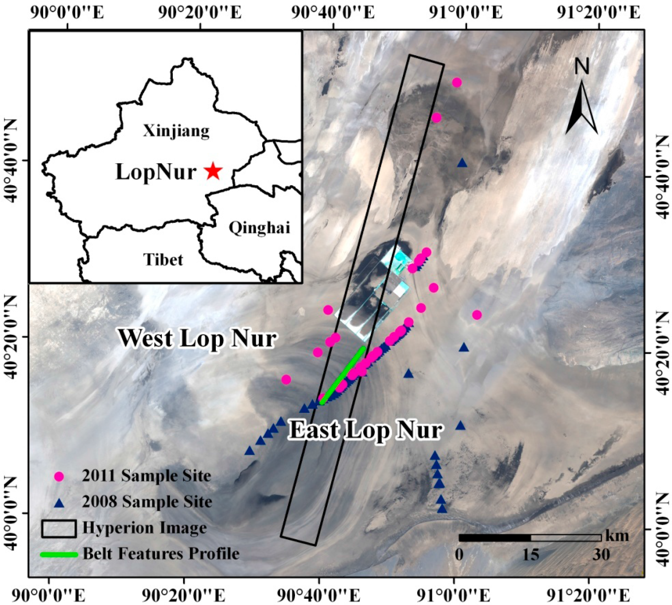
The study area is located in the Lop Nur, Xinjiang, Northwest China. In this region, the annual rainfall is 22 mm, while the evaporation is 3000 mm. There is a strong wind over scale 6 for more than 100 days per year, and the highest air temperature in the summer fluctuates between 40 and 50 °C [3]. The rivers entering Lop Nur have had zero flow in recent years. Due to the special geographical position and climatic condition of Lop Nur, the salt concentration of the crust has varied little since the crust formed.
A total of six field trips were carried out from 2006 to 2011 for visiting to the ruins of the Loulan Kingdom and the Lop Nur Lake region. Among these field trips, samples collected in November 2008 and November 2011 were used for modeling salt-crust properties in this study. These sampling sites were projected onto a georeferenced Landsat TM5 image of the area (Figure 1). In 2008 field trip, three routes, four study areas, and 78 sampling sites were selected along a profile length of a 62 km transect. Each sample collected in 2008 was analyzed for total salt, moisture content, Na+, and Ca2+. From the field work in 2011, a total of 78 surface (0–2 cm) crust samples were collected were used for laboratory spectral measurement and model building. Each of these samples was collected from an approximately 30 × 30 m area. The geographic coordinates of each sampling site were recorded at one-meter accuracy using a global positioning system (GPS) instrument. The samples were kept fresh in sealed plastic bags (17 cm × 20 cm) and transported to laboratory for analysis. Each sample collected in 2011 was analyzed for total slat, Na+, Ca2+, Mg2+, Fe2+, and Si2+.
2.2. Spectral Reflectance Analysis
2.2.1. Satellite Image Spectra
The Hyperion imaging spectrometer is on board the NASA EO-1 satellite, which was launched on 21 November 2000. Hyperion images are characterized by a total of 242 channels at 10-nm spectral intervals over the spectral region 356–2577 nm, acquired at 30 m spatial resolution with an approximate 50:1 signal-to-noise ratio (SNR). A Hyperion scene has 7.7 km cross-track width with 42 or 185 km along-track length. Out of the 242 collected channels, bands 1–7 (356 to 417 nm), bands 58–70 (collected by the VNIR instrument), bands 71–76 (collected by the SWIR instrument), and bands 225–242 (2406 to 2577 nm) are not calibrated. Therefore, a Hyperion image spectrum has total 198 bands from 427 to 2395 nm for further analysis.
One Hyperion image covering part of the study region was acquired on 8 January 2007 with cloud-free. Due to of the difficulty of acquiring satellite hyperspectral data, and especially the weather conditions which are not favorable for conducting field work in Lop Nur in an “ideal” timeline, sampling could not be conducted simultaneously with image data collection. This Hyperion image was the most optimal data for this work, though it did not cover all 2008 and 2011 sampling sites.
The acquired Hyperion image was downloaded from the United States Geological Survey (USGS) website [28] in radiance. Radiometric and geometric corrections were required so that reflectance spectra could be derived from the radiance data and then related to a specified crust property. At the beginning of the preprocessing, uncalibrated image bands and overlay bands were eliminated. The radiance data were converted into surface reflectance using ACORN, a commercial software package for atmospheric calibration. The positional, atmospheric, and weather parameters (i.e., satellite acquisition altitude, humidity, and visibility) required by atmospheric correction. For geometric calibration, the Hyperion image was rectified by referring to a Landsat TM 5 image acquired in 23 August 2007. 39 pairs of ground control point (GCP) were manually selected from the reference TM and the Hyperion image. A bilinear warping method was used to project the Hyperion image into the Universal Transverse Mercator (UTM) coordinates, Zone 46, WGS-84 Datum. Registration accuracy was assessed using the ENVI dynamic overlay function.
Because several noisy bands were corrupted by atmospheric water absorption, these noisy bands were excluded, and 156 bands were retained for partial least squares regression.
2.2.2. Laboratory Spectra
Crushed salt-crust samples were scanned in laboratory using an SVC HR-1024 high-resolution field portable spectroradiometer with the wavelength range 350–2500 nm. A 50-Watt ASD Pro lamp (Analytical Spectral Devices, Boulder, CO, USA) was used as artificial illumination with approximate 30° zenith angle. The fiber-optical head of the spectrometer pointed at the nadir viewing angle at a height of 30 cm above the sample surface. An 8° fore-optic was used, resulting in a 4.2-cm diameter field of view (FOV). Spectral measurement began by scanning a white Spectralon reference panel from Labsphere. Three spectra were acquired for each salt crust sample by rotating the sample by 120° for the second and third measurements. To reduce the effect of salt crust texture on the measured spectra, the average of three spectral measurements for each sample was used in spectral-composition modeling. Because of the SVC sensor, the raw data have two overlapping bands at 983–1019 and 1879–1927 nm. The 978–1015 and 1867–1906 nm bands were therefore removed, leaving 897 bands for modeling.
To compare results for laboratory spectra with those for Hyperion spectra, the spectral bands and crust samples for both datasets must match each other. The laboratory spectra were, therefore, resampled to the Hyperion spectral resolution, resulting in 156 bands from 436 to 2356 nm.
2.3. Partial Least Squares (PLS) Modeling
Partial least squares (PLS) modeling was used to build relationships between salt crust parameters and hyperspectral data. PLS is a standard multivariate regression method developed by Herman Wold [29,30]. PLS uses a few eigenvectors of the explanatory variables so that the corresponding scores not only explain the variance in the explanatory variables, but also have high correlations with the response variables. A simplified PLS model consists of the two outer relations shown in Equations (1) and (2), which describe the eigenstructure decomposition of both the matrix containing the explanatory variables (i.e., spectral bands) and the matrix containing the response variables (i.e., the abundance of Ca2+), and an inner relation shown in Equation (3), which links the score matrices resulting from these two eigenstructure decompositions [31]:
The first outer relation is derived by applying principal component analysis (PCA) to X, resulting in the score matrix T and the loading matrix D plus an error matrix E. In a similar way, the second outer relation is derived by decomposing Y into the score matrix U, the loading matrix Q, and the error term F. The inner relation is a multiple linear regression between the score matrices U and T in which B is a regression coefficient matrix determined by least-squares minimization. The prime (′) represents a matrix transpose. Y is computed as:
The goal of PLS modeling is to minimize the norm of F while maximizing the covariance between X and Y by the inner relationship. Because the two separate PCA approaches to the derivation of PLS factors described above are not the best possible ones and could result in a weak correlation for the inner relation, a method resulting in a strong inner relation between T and U was used in this study [31–33]. Selecting the optimal number of latent variables is essential for building a robust PLS model. The leave-one-out cross-validation method was used to determine the optimal number of latent variables. Given a set of m samples, m-1 samples are used to develop a calibration model, and the concentration of the left-out sample is predicted using the calibration model. This process is repeated until each sample has been excluded once. The predicted error sum of squares (PRESS) can be calculated as:
For a specified salt crust property parameter, two statistical indices, the leverage and the Studentized residual, were used to determine outliers [33]. The identified outliers were discarded from PLS analysis. In PLS analysis, the dataset was divided into two subsets: one for calibration, and the other for validation. 30% of the samples were randomly selected as the validation dataset. The leave-one-out cross-validation method was used to determine the optimal number of PLS factors.
Previous studies have shown that data pretreatment improves PLS performance [32,34]. Mean centering was used in this study. Mean centering subtracts the means of individual spectral bands from the spectral data; similar subtractions were applied to salt-crust property values. Mean centering was used because it is simple and facilitates the interpretation of PLS results.
Prediction accuracy was assessed on the basis of the coefficient of determination (R2), the slope (b) of the regression line, and the root mean square errors of calibration dataset (RMSEC) and validation dataset (RMSEP). The ratio of performance deviation (RPD) was also used to evaluate prediction accuracy. RPD is the ratio of the standard deviation (SD) of a sample chemical concentration to root mean square error (RMSE) from a PLS model [35]. Many researchers have used RPD to evaluate the stability and effectiveness of PLS calibration and prediction [36–39]. Here, RPD was used as proposed by Chang et al. [24]: results from PLS modeling were classified as good if RPD > 2, as satisfactory and open to improvement using different calibration strategies if 1.4 ≤ RPD ≤ 2, and as unreliable if RPD < 1.4.
3. Results and Discussions
3.1. Properties of Laboratory Spectra
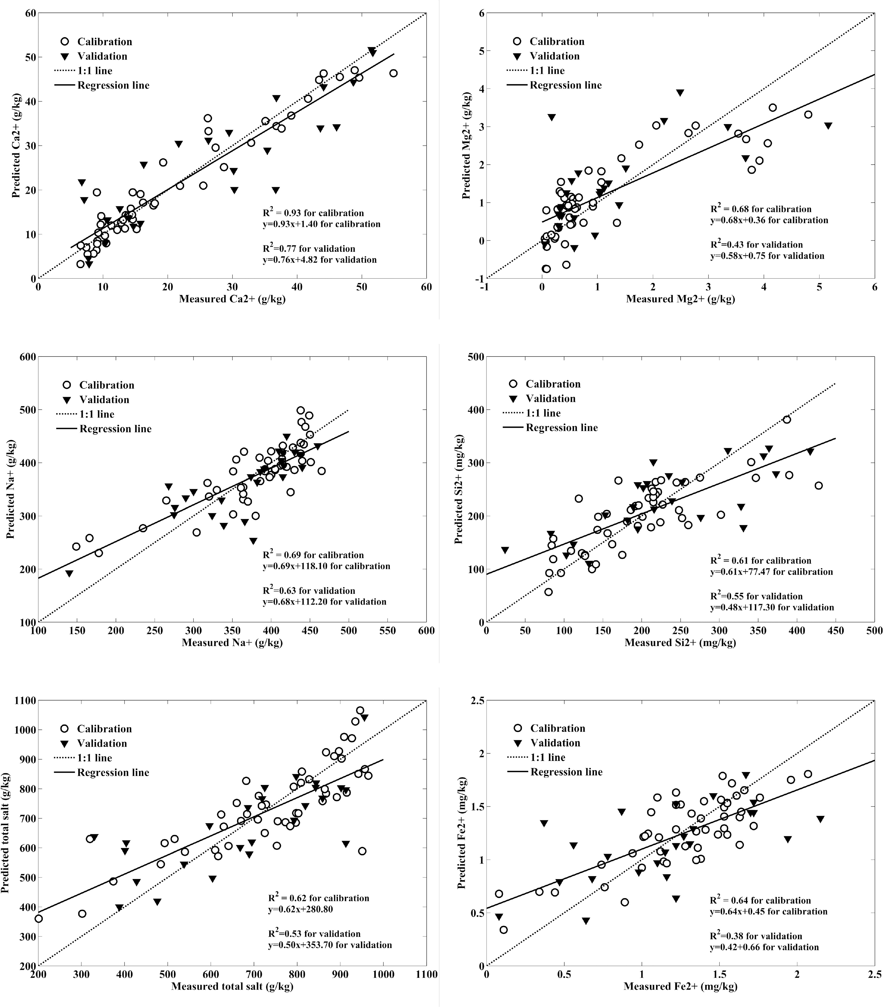
A total of 78 samples were analyzed for the laboratory spectra, of which three samples were identified as outliers and 75 samples were used in PLS modeling. Twenty-five of these samples were randomly selected for validation, and 50 remaining samples were used for calibration to estimate individual salt-crust property contents. Table 1 lists the chemical content ranges of both the calibration and the validation datasets and the number of samples in each dataset. From Table 1, it can be seen that there were no significant differences between both datasets for any of the salt-crust property parameters when mean contents were compared. The standard deviations of soil samples for both calibration and validation were similar for all the properties examined. PLS modeling was conducted with measured and simulated Hyperion spectra, with the results summarized in Table 2, Figures 2 and 3.
Both R2 and RPD values indicated that Ca2+ can be estimated using laboratory spectra at different spectral resolutions, with R2 ≥ 0.88 and RPD > 2. These results are expected and consistent with previous studies which show that Ca2+ can be reliably estimated from lab measured reflectance spectra [24,40,41]. PLS resulted in good estimation with laboratory spectra for Fe2+ and Si2+ with R2 ≥ 0.87 and RPD > 2. These findings are similar to those of Cozzolino et al. [40]. PLS performed satisfactory estimation with laboratory spectra for total salt, Mg2+, and Na+ with 2 > RPD > 1.4. The calibrations for total salt and Na with laboratory data were not as good as for the other properties, but satisfactory nonetheless. In terms of R2, our result for Na+ is better than R2 of 0.09 reported by Chang et al. [24]. PLS with the simulated Hyperion spectra yielded accurate estimates for total salt, Mg2+, and Na+ and satisfactory estimates for Fe2+ and Si2+, with 2 > RPD > 1.4. For Fe2+ and Si2+, R2 and RPD values with simulated Hyperion data were lower than those resulting from PLS with 897-band laboratory spectra, suggesting the lower spectral resolution decreased estimation accuracy.
In general, the validation results indicated that PLS can satisfactorily predict most of salt-crust properties from hyperspectral data. All RPD values for PLS validation were less than 2 except for Ca2+ with simulated Hyperion spectra, implying that almost no soil properties can be predicted using hyperspectral data with good accuracy. The PLS models with the laboratory spectra (897 bands) and the simulated Hyperion spectra produced satisfactory validation for total salt, Na+ and Si2+. PLS gave the poorest prediction for Mg2+ using the laboratory data and simulated Hyperion data. The result is not consistent with the results reported by Shepherd et al. [41]. The reason maybe attributed to the Mg2+ range of the validation samples. The calibration dataset and validation dataset both were selected randomly. The Mg2+ range for the calibration dataset is 0.049–4.80 g/kg, while the Mg2+ range for the validation dataset is 0.048–5.60 g/kg. The Mg2+ range for validation is beyond the range for calibration.
The two datasets were different in spectral resolution. The spectral resolution of the 897-band laboratory spectrum dataset was 2 nm, whereas the spectral resolution of the 156-band simulated Hyperion spectral dataset was 10 nm. PLS performance for these two datasets was compared. The effects of spectral resolution on PLS performance in predicting soil properties were evaluated based on the coefficient of determination (R2) and the RPD values resulting from validation (Table 2). PLS with simulated Hyperion spectra resulted in more accurate estimates (RPD = 3.91) and validation (RPD = 2.11) for Ca2+ than PLS with laboratory data (Table 2). PLS performance for predicting these properties was not sensitive to the degraded spectral resolution.
3.2. Hyperion Spectra of Ca2+ Property and Mapping Results
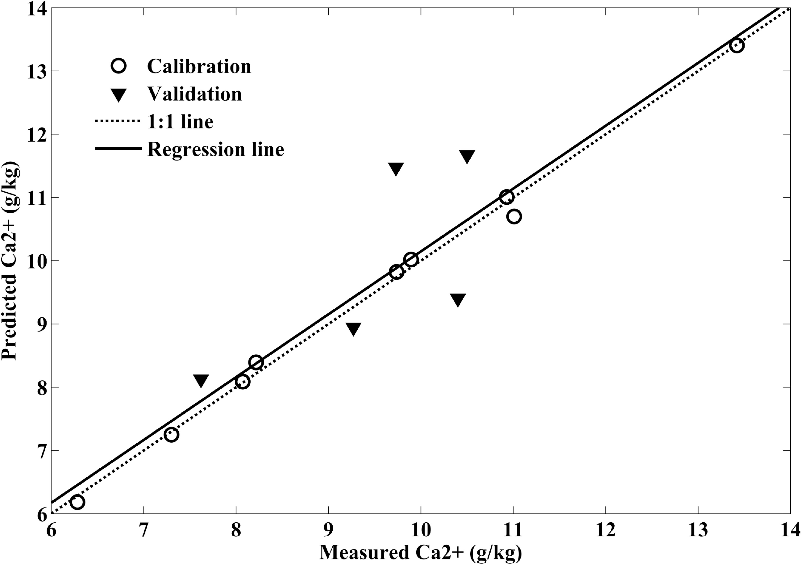
To obtain the Ca2+ distribution around the “ear” area, Hyperion image spectra were used to build the relationship with Ca2+ abundance. Because of special environmental conditions in Lop Nur, the Ca2+ concentration of the crust changed little without eluviation. This means that a Hyperion image acquired in 2007 can be used to estimate the Ca2+ distribution since then. Salt-crust samples were collected in 2008 and 2011. A total of 13 samples were covered by the Hyperion image. Eight samples from 2008 were used for calibration and five samples from 2011 for validation. The PLS results for the Hyperion image spectrum demonstrated good calibration for Ca2+, with R2 = 0.99 and RPD > 13.48, and satisfactory validation, with R2 = 0.51, RPD > 1.72 (Figure 4). These results are comparable to the findings by Lagacherie et al. [42], who reported that stable estimation for calcium carbonate using airborne HYMAP image spectra. These results demonstrate that Ca2+ of salt-crust for playa lake could be mapped with spaceborne hyperspectral imagery.
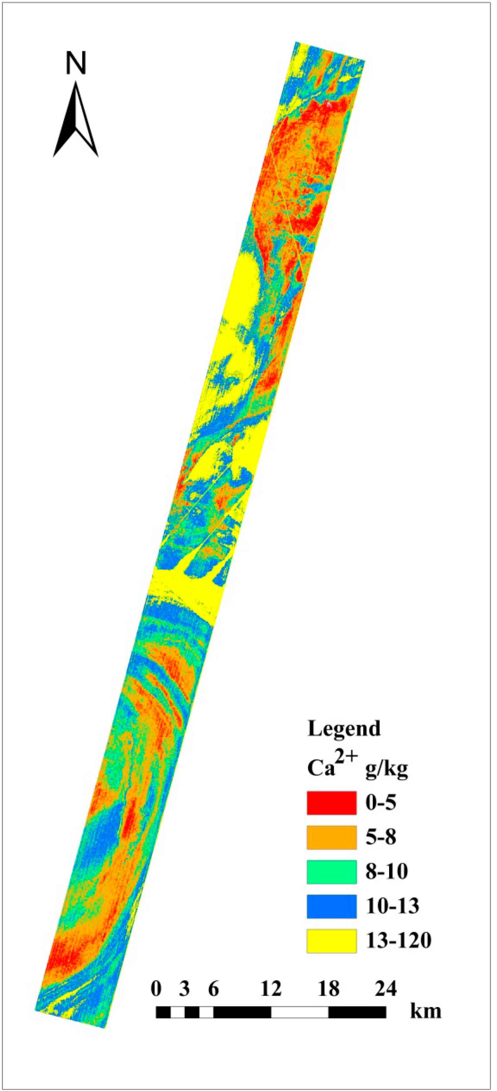
The PLS model with 13 salt-crust samples was applied to the Hyperion images to generate a spatial distribution map of Ca for the Lop Nur “ear” area. The Ca2+ distribution for “ear” area on the map is dominated by an orange color with 5%–8% Ca2+ (Figure 5). The blue belt represents 10%–13% Ca2+ as seen on the map.
3.3. Relationship between Ca2+ Abundance and Belt Features
The belt features of the Lop Nur lake region appear as “a big ear” in remote sensing images. The mean value of reflectance from the first three TM bands (TM 1: 450–520 nm, TM 2: 520–600 nm, TM 3: 620–690 nm) was used to express the belt characteristic that light rings alternate with dark rings with roughly circular distribution. Ca2+ distribution was compared to the texture feature of the “Ear area” shown in the TM image to explain the formation process and the environmental meanings of the belt features.
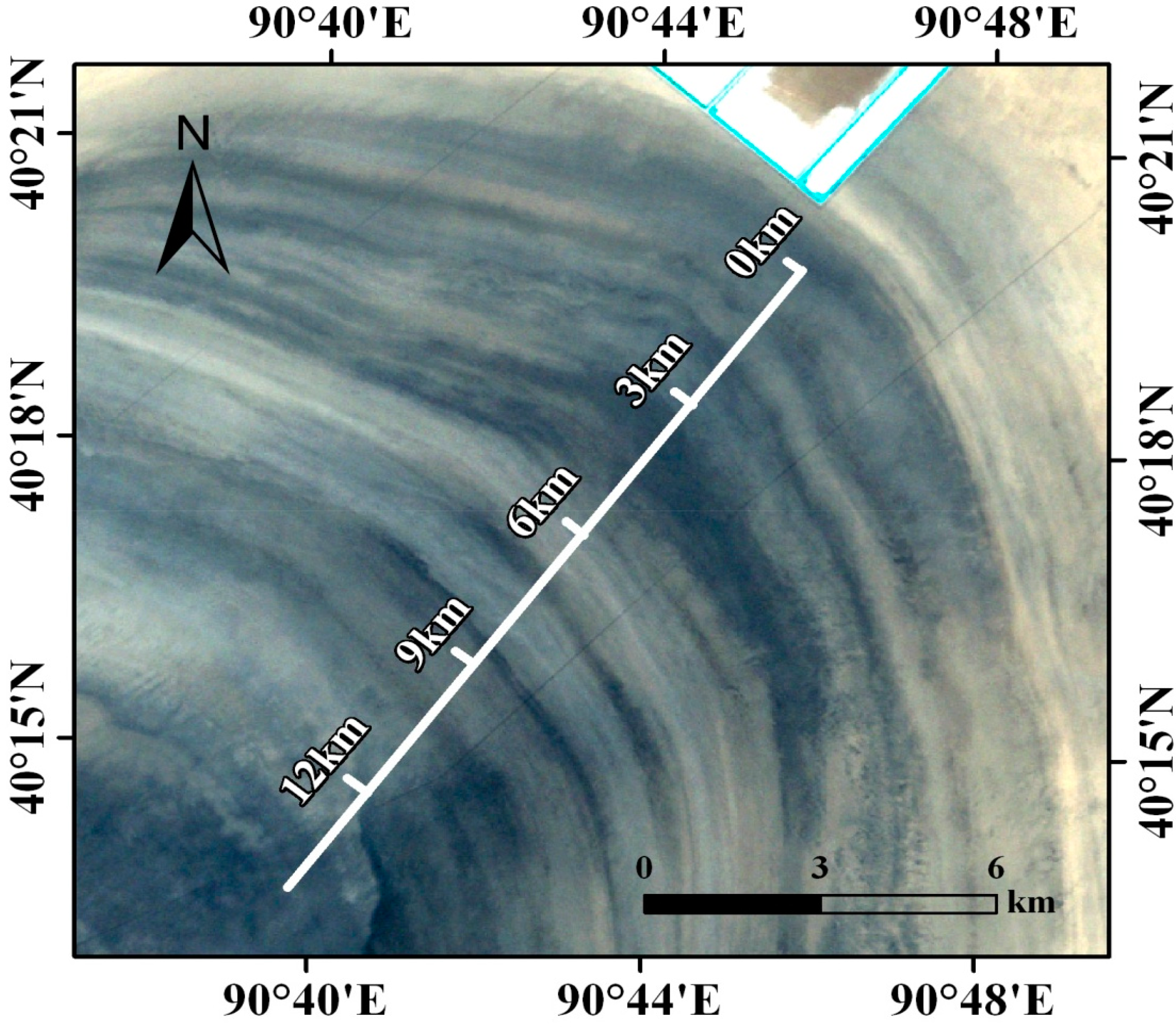
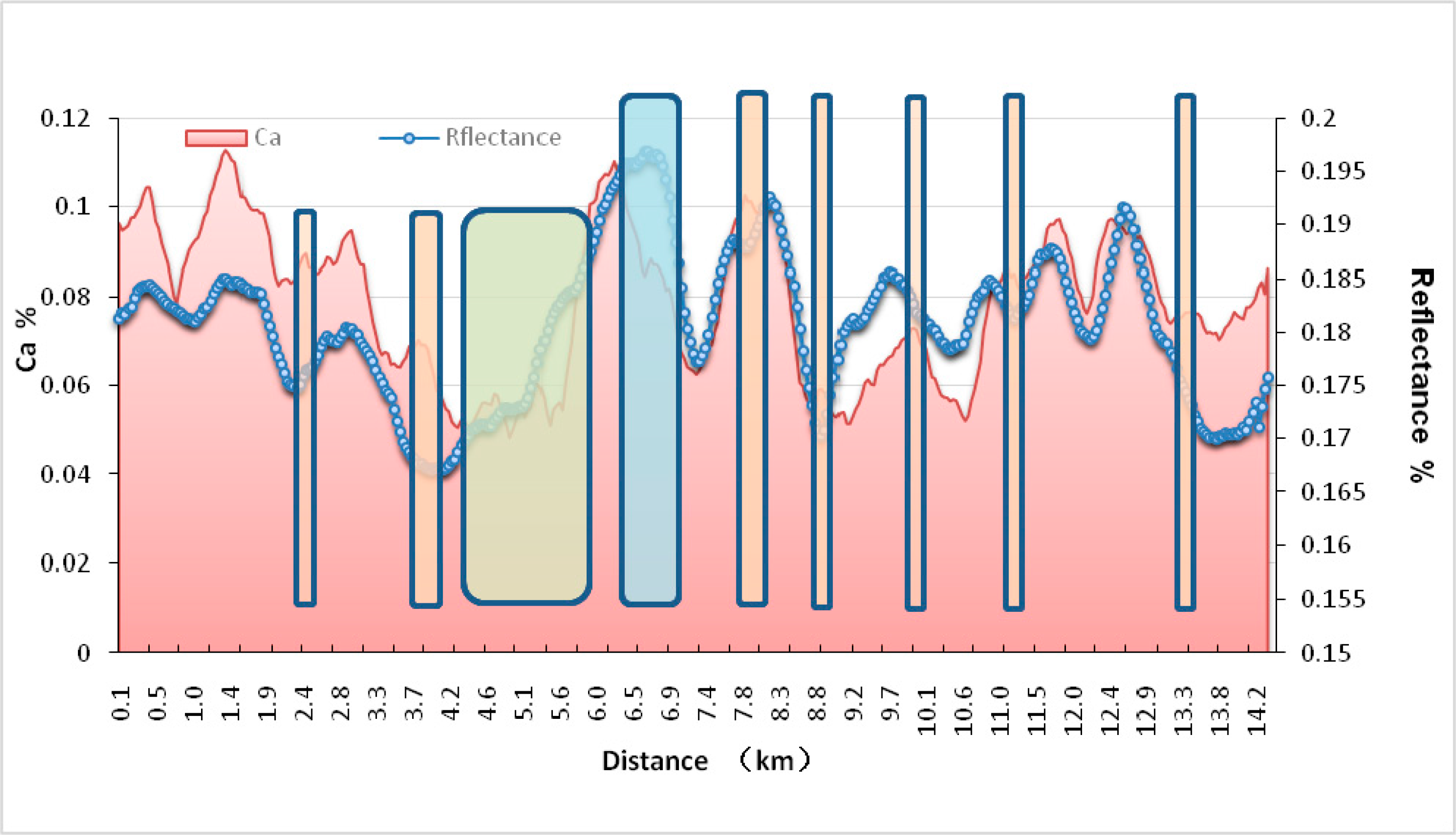
A transversal profile of 14 km (Figure 6) to the rings of the “ear” was drawn to extract the reflectance of each ring from the TM image. The corresponding Ca2+ distribution for this 14-km-long profile was obtained from the mapping results for the Hyperion image. Comparison between Ca2+ content and reflectance is shown in Figure 7, and their variations are consistent. In the Lop Nur Lake region, Ca2+ generally exists in gypsum (CaSO4), and gypsum is a deposited material indicative of an arid environment. During the dry period of a saline lake, with ongoing lake retreat, salt will continue to deposit. The reflectance of salt is higher than that of deposited sediments. The amount of salt deposition therefore has a positive correlation with reflectance. Variation of Ca2+ content was consistent with salt deposition. The correlation between Ca2+ content and reflectance was in accordance with salt-lake evolution.
Moreover, some anti-correlated areas shown in Figure 7 can be used to explain the environmental background of the belt features. At two anti-correlated areas at 2.4 and 3.7 km, Ca2+ content reaches peak values, and the corresponding reflectance values are in valley. Large values of Ca2+ deposition readings show that the climate was arid, whereas the low reflectance indicated that temporary larger upstream runoff events, carrying large quantities of sediments, may occur. These two anti-correlated areas should belong to the same climatic period because of their close location, when some extreme weather events perhaps occurred to cause unstable upland water flow. From 4.2 to 5.6 km, Ca2+ content shows a consistent trend with variation in reflectance, but the stability is poor, indicating that this period could represent the unstable transition period during a drought. From 6.5 to 6.9 km, Ca2+ content decreases, and reflectance increases; with less upland water flow, the salt concentration of the lake was probably so high that Ca2+ precipitation gradually weakened and then Na and K as high-solubility salts began to precipitate and deposit. This period could have been one of extreme droughts. At the anti-correlated areas at 7.9, 8.9, 10.0, 11.1, and 13.4 km, Ca2+ content has negative correlation with reflectance, indicating that there could have been a small-scale temporary runoff event under an arid environmental background, leading to a temporary increase in sediment and making the reflectance of these areas low.
From 8.9–14 km, four narrow abnormal domains can be observed, indicating small-scale temporary runoff events. During the late stage of playa-lake evolution, because of the small quantity of lake water, sediment deposition was sensitive to upland water supply. It is not yet possible to determine whether these areas of small-scale runoff are due to natural factors (climate events) or human factors (upstream channel changes). Further work is needed to date the various belts and combine them with modern hydrological data to synthesize an analysis.
4. Conclusions
In this paper, PLS models estimating playa lake crust constituents: total salt, Ca2+, Mg2+, Na+, Si2+, and Fe2+ are developed using laboratory hyperspectral data with high and low spectral resolution. Validation results prove that most of the studied salt-crust properties can be predicted with satisfactory accuracy using hyperspectral data. A Ca2+ abundance map is derived by applying the PLS model to the Hyperion image. A transversal profile of 14 km to the rings of the “ear” was drawn to extract reflectance of each ring from the Landsat TM image. Comparison results between Ca2+ content and reflectance show that the Ca2+ content has positive correlation with reflectance, and their variations are consistent. Variation of Ca2+ content was consistent with salt deposition. The correlation between Ca2+ content and reflectance was in accordance with salt-lake evolution. The presence of some anti-correlated areas may indicate the occurrence drought periods or small-scale temporary runoff events. What needs to be mentioned is that small-scale runoff events need further work to determine.
Acknowledgments
The authors are grateful to several institutions for support for sampling, experiments, and data interpretation. This work was supported by the CAS Knowledge Innovation Program (KZCX2-EW-320), National Natural Science Foundation of China (41301394, 41201346, U1303285, 41301464), Key technology studies on soil and water environmental parameters in Qinghai Lake watershed (Grant No. 2012BAH31B02-03) provided by the Department of Science and Technology of Qinghai Province, the fund of the State Key Laboratory of Remote Sensing Science (Y1Y00201KZ), and major special industry application projects (05-Y30B02-9001-13/15-03).
Author Contributions
Tingting Zhang was responsible for developing PLS models estimating playa lake crust constituents with hyperspectral data, applying PLS model to Hyperion image, and analysis on the relationship between Ca2+ abundance and belt features, in addition to reviewing the final manuscript. Yun Shao provided guidance of evolution of Lop Nur Lake basin. Huaze Gong analyzed the environmental meanings of Ca2+ variation. Lin Li was responsible for analyzing PLS results, and he also checked the description of this paper in order to make it to be understood better for readers. Longfei Wang plotted all the figures in this paper and took part in some works of data analysis.
Conflicts of Interest
The authors declare no conflict of interest.
References
- Xia, X.; Wang, F.; Zhao, Y. Lop Nur in China; Science Press: Beijing, China, 2007. [Google Scholar]
- Zhang, J.; Liu, C.; Wu, X.; Liu, K.; Zhou, L. Optically stimulated luminescence and radiocarbon dating of sediments from Lop Nur (Lop Nor), China. Quat. Geochronol 2012, 10, 150–155. [Google Scholar]
- Luo, C.; Peng, Z.; Yang, D.; Liu, W.; Zhang, Z.; He, J.; Chou, C. A lacustrine record from Lop Nur, Xinjiang, China: Implications for paleoclimate change during Late Pleistocene. J. Asian Earth Sci 2009, 34, 38–45. [Google Scholar]
- Gong, H.; Shao, Y.; Zhang, T.; Liu, L.; Wang, G. Scattering mechanisms for the “Ear” feature of Lop Nur lake basin. Remote Sens 2014, 6, 4546–4562. [Google Scholar]
- Dong, Z.; Lv, P.; Qian, G.; Xia, X.; Zhao, Y.; Mu, G. Research progress in China’s Lop Nur. Earth Sci. Rev 2012, 111, 142–153. [Google Scholar]
- Shao, Y.; Gong, H.; Gao, Z.; Liu, L.; Zhang, T. SAR data for subsurface saline lacustrine deposits detection and primary interpretation on the evolution of the vanished Lop Nur Lake. Can. J. Remote Sens 2012, 38, 267–280. [Google Scholar]
- Fan, Z.; Li, P.; Zhang, B. Scientific Exploration and Study of the Lop Nur; Science Press: Beijing, China, 1987. [Google Scholar]
- Lin, J.; Zhang, J.; Ju, Y.; Wang, Y.; Lin, F.; Zhang, J.P.; Wang, S.; Wei, M. The lithostratigraphy, magnetostratigraphy, and climatostratigraphy in the Lop Nur region, Xinjiang. J. Stratigr 2005, 29, 317–322. [Google Scholar]
- Luo, C.; Yang, D.; Peng, Z. Multi-proxy evidence for late Pleistocene-Holocene climatical and environmental change in Lop-Nur, Xinjiang, NW China. Chin. J. Geochem 2008, 27, 257–264. [Google Scholar]
- Zhu, Q.; Wang, F.; Cao, Q.; Xia, X.; Li, S.; Ma, C. Grain size distribution characteristics and changes of Lop Nur Lake druing the past 10,000 years. J. Stratigr 2009, 33, 283–290. [Google Scholar]
- Cai, A.M.; Shao, Y.; Gong, H.Z.; Wang, G.J.; Xie, C. Analysis of Lop Nur “Ear” features in remote sensing image and its environmental meaning. Spectrosc. Spectr. Anal 2011, 31, 1633–1638. [Google Scholar]
- Allbed, A.; Kumar, L.; Sinha, P. Mapping and modelling spatial variation in soil salinity in the Al Hassa Oasis based on remote sensing indicators and regression techniques. Remote Sens 2014, 6, 1137–1157. [Google Scholar]
- Asner, G.P.; Heidebrecht, K.B. Imaging spectroscopy for desertification studies: Comparing AVIRIS and EO-1 Hyperion in Argentina drylands. IEEE Trans. Geosci. Remote Sens 2003, 41, 1283–1296. [Google Scholar]
- Ben-Dor, E.; Banin, A. Near-infrared reflectance analysis of carbonate concentration in soils. Appl. Spectrosc 1990, 44, 1064–1069. [Google Scholar]
- Ben-Dor, E.; Banin, A. Visible and near-infrared (0.4–1.1 μm) analysis of arid and semiarid soils. Remote Sens. Environ 1994, 48, 261–274. [Google Scholar]
- Bogrekci, I.; Lee, W.S. Spectral soil signatures and sensing phosphorus. Biosyst. Eng 2005, 92, 527–533. [Google Scholar]
- Ingleby, H.R.; Crowe, T.G. Reflectance models for predicting organic carbon in Saskatchewan soils. Can. Agric. Eng 2000, 42, 57–63. [Google Scholar]
- Palacios-Orueta, A.; Ustin, S.L. Remote sensing of soil properties in the Santa Monica Mountains I. Spectral analysis. Remote Sens. Environ 1998, 65, 170–183. [Google Scholar]
- Schwanghart, W.; Jarmer, T. Linking spatial patterns of soil organic carbon to topography—A case study from south easten Spain. Geomorphology 2011, 126, 252–263. [Google Scholar]
- Thomasson, J.A.; Sui, R.; Cox, M.S.; Al-Rajehy, A. Soil reflectance sensing for determining soil properties in precision agriculture. Trans. ASAE 2001, 44, 1445–1453. [Google Scholar]
- Zhang, T.; Li, L.; Zheng, B. Estimation of agricultural soil properties with imaging and laboratory spectroscopy. J. Appl. Remote Sens 2013, 7. [Google Scholar] [CrossRef]
- Gmur, S.; Vogt, D.; Zabowski, D.; Moskal, M. Hyperspectral analysis of soil nitrogen, carbon, carbonate, and organic matter using regression trees. Sensors 2012, 12, 10639–10658. [Google Scholar]
- Mougenot, B.; Epema, G.F.; Pouget, M. Remote sensing of salt affected soils. Remote Sens. Environ 1993, 7, 241–259. [Google Scholar]
- Chang, C.W.; Laird, D.A.; Mausbach, M.J.; Hurburgh, C.R. Near infrared reflectance spectroscopy-principal components regression analyses of soil properties. Soil Sci. Soc. Am J 2001, 65, 480–490. [Google Scholar]
- Dunn, B.W.; Beecher, H.G.; Batten, G.D.; Ciavarella, S. The potential of near-infrared reflectance spectroscopy for soil analysis—A case study from the Riverine Plain of south-eastern Australia. Aust. J. Exp. Agric 2002, 42, 607–614. [Google Scholar]
- Crowley, J.K. Mapping playa evaporit minerals with AVIRIS data: A first report from Death Valley, California. Remote Sens. Environ 1993, 44, 337–356. [Google Scholar]
- Kodikara, G.R.L.; Woldai, T.; van Ruitenbeek, F.J.A.; Kuria, Z.; van der Meer, F.; Shepherd, K.D.; van Hummel, G.J. Hyperspectral remote sensing of evaporate minerals and associated sediments in Lake Magadi area, Kenya. Int. J. Appl. Earth Obs. Geoinf 2012, 14, 22–32. [Google Scholar]
- USGS Global Visualization Viewer. Available online: http://glovis.usgs.gov (accessed on 24 June 2014).
- Wold, H. Nonlinear estimation by eterative least squares procedure. In Research Papers in Statistics; David, F.N., Neyman, J., Eds.; Wiley: New York, NY, USA, 1966; pp. 441–444. [Google Scholar]
- Wold, H. Estimation of principal components and related models by iterative lease squares. In Multivariate Analysis; Krishnaiah, P.R., Ed.; Elsevier: New York, NY, USA, 1966; pp. 391–420. [Google Scholar]
- Geladi, P.; Kowalski, B.R. Partial least-squares regression: A tutorial. Anal. Chim. Acta 1986, 185, 1–17. [Google Scholar]
- Haaland, D.M.; Thomas, E.V. Partial least-squares methods for spectral analyses. 1. Relation to other quantitative calibration methods and the extraction of qualitative information. Anal. Chem 1988, 60, 1193–1202. [Google Scholar]
- Martens, H.; Næs, T. Multivariate Calibration; John Wiley and Sons: Hoboken, NJ, USA, 2002. [Google Scholar]
- Azzouza, T.; Puigdoménechb, A.; Aragay, M.; Tauler, R. Comparison between different data pre-treatment methods in the analysis of forage samples using near-infrared diffuse reflectance spectroscopy and partial least-squares multivariate calibration method. Anal. Chim. Acta 2003, 484, 121–134. [Google Scholar]
- Nduwamungu, C.; Ziadi, N.; Parent, L.-E.; Tremblay, G.F.; Thuriès, L. Opportunities for, and limitations of, near infrared reflectance spectroscopy applications in soil analysis: A review. Can. J. Soil Sci 2009, 89, 531–541. [Google Scholar]
- Brown, D.J.; Bricklemyer, R.S.; Miller, P.R. Validation requirements for diffuse reflectance soil characterization models with a case study of VNIR soil C prediction in Montana. Geoderma 2005, 129, 251–267. [Google Scholar]
- Du, C.; Zhou, J.; Wang, H.; Chen, X.; Zhu, A.; Zhang, J. Determination of soil properties using Fourier transform mid-infrared photoacoustic spectroscopy. Vib. Spectrosc 2009, 49, 32–37. [Google Scholar]
- Gomez, C.; Viscarra Rossel, R.A.; McBratney, A.B. Soil organic carbon prediction by hyperspectral remote sensing and field vis-NIR spectroscopy: An Australian case study. Geoderma 2008, 146, 403–411. [Google Scholar]
- Willams, P.C.; Sobering, D.C. Comparison of commercial near infrared transmittance and reflectance instuments for analysis of whole grains and seeds. J. Near Infrared Spectrosc 1993, 1, 25–32. [Google Scholar]
- Cozzolino, D.; Moron, A. The potential of near-infrared reflectance spectroscopy to analyse soil chemical and physical charactreristics. J. Agric. Sci 2003, 140, 65–71. [Google Scholar]
- Shepherd, K.D.; Walsh, M.G. Development of reflectance spectral libraries for characterization of soil properties. Soil Sci. Soc. Am. J 2002, 66, 988–998. [Google Scholar]
- Lagacherie, P.; Baret, F.; Feret, J.B.; Netto, J.M.; Robbez-Masson, J.M. Estimation of soil clay and calcium carbonate using laboratory, field and airborne hyperspectral measurements. Remote Sens. Environ 2008, 112, 825–835. [Google Scholar]


| Parameter | Number of Samples | Minimum Content | Maximum Content | Mean Content | Standard Deviation |
|---|---|---|---|---|---|
| Calibration samples | |||||
| Ca2+ (g/kg) | 50 | 6.52 | 54.90 | 20.99 | 13.72 |
| Total salt (g/kg) | 50 | 201.00 | 965.00 | 736.48 | 183.28 |
| Mg2+ (g/kg) | 50 | 0.049 | 4.80 | 1.12 | 1.32 |
| Na+ (g/kg) | 50 | 149.00 | 465.00 | 378.32 | 72.59 |
| Fe2+ (mg/kg) | 50 | 0.08 | 2.07 | 1.26 | 0.42 |
| Si2+ (mg/kg) | 50 | 80.00 | 428.00 | 199.88 | 82.09 |
| Validation samples | |||||
| Ca2+ (g/kg) | 25 | 6.73 | 51.70 | 26.26 | 15.50 |
| Total salt (g/kg) | 25 | 330.00 | 956.00 | 679.52 | 190.32 |
| Mg2+ (g/kg) | 25 | 0.048 | 5.16 | 1.20 | 1.26 |
| Na+ (g/kg) | 25 | 140.00 | 460.00 | 363.24 | 73.55 |
| Fe2+ (mg/kg) | 25 | 0.08 | 2.15 | 1.15 | 0.51 |
| Si2+ (mg/kg) | 25 | 24.00 | 417.00 | 227.64 | 99.21 |
| Soil Properties | Data Type | NLv | Calibration | Validation | ||||
|---|---|---|---|---|---|---|---|---|
| Rc2 | RPDc | RMSEC | Rv2 | RPDv | RMSEP | |||
| Ca2+ (g/kg) | Laboratory | 7 | 0.88 | 2.89 | 4.75 | 0.73 | 1.95 | 7.95 |
| simulated Hyperion | 10 | 0.93 | 3.91 | 3.51 | 0.77 | 2.11 | 7.33 | |
| Total Salt (g/kg) | Laboratory | 6 | 0.62 | 1.64 | 112.04 | 0.53 | 1.48 | 128.63 |
| simulated Hyperion | 6 | 0.62 | 1.75 | 105.01 | 0.53 | 1.54 | 123.46 | |
| Mg2+ (g/kg) | Laboratory | 5 | 0.93 | 1.39 | 0.95 | 0.44 | 1.09 | 1.16 |
| simulated Hyperion | 5 | 0.68 | 1.78 | 0.74 | 0.43 | 1.26 | 1.00 | |
| Na+ (g/kg) | Laboratory | 5 | 0.64 | 1.68 | 43.10 | 0.56 | 1.51 | 48.85 |
| simulated Hyperion | 6 | 0.69 | 1.81 | 40.16 | 0.63 | 1.66 | 44.33 | |
| Fe2+ (mg/kg) | Laboratory | 8 | 0.87 | 2.77 | 0.15 | 0.18 | 1.07 | 0.48 |
| simulated Hyperion | 6 | 0.64 | 1.69 | 0.25 | 0.38 | 1.29 | 0.40 | |
| Si2+ (mg/kg) | Laboratory | 9 | 0.90 | 3.18 | 25.84 | 0.52 | 1.48 | 67.13 |
| simulated Hyperion | 6 | 0.61 | 1.62 | 50.59 | 0.55 | 1.51 | 65.66 | |
© 2014 by the authors; licensee MDPI, Basel, Switzerland This article is an open access article distributed under the terms and conditions of the Creative Commons Attribution license (http://creativecommons.org/licenses/by/3.0/).
Share and Cite
Zhang, T.; Shao, Y.; Gong, H.; Li, L.; Wang, L. Salt Content Distribution and Paleoclimatic Significance of the Lop Nur “Ear” Feature: Results from Analysis of EO-1 Hyperion Imagery. Remote Sens. 2014, 6, 7783-7799. https://doi.org/10.3390/rs6087783
Zhang T, Shao Y, Gong H, Li L, Wang L. Salt Content Distribution and Paleoclimatic Significance of the Lop Nur “Ear” Feature: Results from Analysis of EO-1 Hyperion Imagery. Remote Sensing. 2014; 6(8):7783-7799. https://doi.org/10.3390/rs6087783
Chicago/Turabian StyleZhang, Tingting, Yun Shao, Huaze Gong, Lin Li, and Longfei Wang. 2014. "Salt Content Distribution and Paleoclimatic Significance of the Lop Nur “Ear” Feature: Results from Analysis of EO-1 Hyperion Imagery" Remote Sensing 6, no. 8: 7783-7799. https://doi.org/10.3390/rs6087783