Classification of Grassland Successional Stages Using Airborne Hyperspectral Imagery

 , ,
, ,
Abstract
: Plant communities differ in their species composition, and, thus, also in their functional trait composition, at different stages in the succession from arable fields to grazed grassland. We examine whether aerial hyperspectral (414–2501 nm) remote sensing can be used to discriminate between grazed vegetation belonging to different grassland successional stages. Vascular plant species were recorded in 104.1 m2 plots on the island of Öland (Sweden) and the functional properties of the plant species recorded in the plots were characterized in terms of the ground-cover of grasses, specific leaf area and Ellenberg indicator values. Plots were assigned to three different grassland age-classes, representing 5–15, 16–50 and >50 years of grazing management. Partial least squares discriminant analysis models were used to compare classifications based on aerial hyperspectral data with the age-class classification. The remote sensing data successfully classified the plots into age-classes: the overall classification accuracy was higher for a model based on a pre-selected set of wavebands (85%, Kappa statistic value = 0.77) than one using the full set of wavebands (77%, Kappa statistic value = 0.65). Our results show that nutrient availability and grass cover differences between grassland age-classes are detectable by spectral imaging. These techniques may potentially be used for mapping the spatial distribution of grassland habitats at different successional stages.1. Introduction
The rationalization of European agricultural landscapes during the last century has resulted in the fragmentation and loss of species-rich semi-natural habitats, leading to a dramatic decrease in farmland biodiversity across Europe [1]. The remaining old fragments of grazed semi-natural grasslands are among the most species-rich habitats within the agricultural landscape [2], and they are of great importance for the overall species richness of agricultural landscapes [3]. As well as agricultural intensification in many areas, there has also been a successive increase in the area of abandoned cultivated land in several parts of Europe over the past 50 years [4]. In many European regions, abandoned arable fields are gradually being transformed into grazed grasslands [5,6]. The majority of the grasslands in the present-day agricultural landscape are grazed fields that represent early stages in the succession from arable cultivation towards species-rich old grasslands [7].
The transformation of abandoned arable land into grazed grassland is expected to offer new possibilities for the establishment of species-rich and diverse grassland vegetation and to mitigate biodiversity loss in agricultural landscapes [8,9]. If species diversity in cultivated landscapes is to be maintained and enriched in the future, species will need to be able to disperse from old, species-rich grassland fragments into younger grasslands [10]. Optimization of the spatial distribution of grassland fragments will require information that discriminates between land cover belonging to different stages in the succession from arable fields to old semi-natural grasslands. It may be difficult to collect explicit spatial information on grassland age and habitat characteristics over wide areas solely from field-based assessments [11]. Field-based inventories of grasslands are time consuming and are therefore often based on plot-scale sampling within spatially restricted areas (cf. [12]).
Remote sensing technology has the ability to support and supplement field-based habitat inventories [13,14], and the potential of remote sensing data as a source of information both within vegetation science [15] and as a tool within conservation biology has recently been highlighted [16]. The development of remote sensing-based methods that can be used for the mapping of habitats at detailed scales is considered to be particularly important [16]. Aerial photographs and broadband satellite-based spectral data have been used to map and monitor grassland properties. For example, Waldhardt and Otte [17] showed that grassland vegetation of different ages could be discriminated with the help of the colour tonal values from false-colour infrared aerial photographs. Kawamura et al. [18] used spectral information acquired from satellite data to assess grazing intensity in grasslands. However, the low spectral resolution of aerial photographs and broad-band sensors limits the collection of detailed information on vegetation properties [19,20].
Hyperspectral remote sensing (imaging spectroscopy) is a particularly good method for assessing and monitoring vegetation characteristics [21–23]. Spectral measurements acquired by hyperspectral sensors provide detailed information on the structural and biochemical properties of vegetation [24,25]. For example, plant functional traits and properties, such as leaf nitrogen content, leaf chlorophyll content, leaf water content, and leaf area index, have been successfully estimated with the help of hyperspectral data [26–29]. Ecological indicators, such as Ellenberg values [30], are commonly used to describe relationships between vegetation and environment [31]. Schmidtlein [12] mapped gradients of community-weighted mean Ellenberg indicator values for nutrient and moisture availability in montane pastures, and Klaus et al. [32] predicted mean Ellenberg indicator values for nutrient and moisture availability in agricultural grasslands using spectroscopy data.
Previous studies have shown that grassland plant communities representing different stages in the arable-to-grassland succession are characterized by different habitat conditions and plant community characteristics [33,34]. Old grasslands have lower community-weighted mean values for Ellenberg indicators for nutrient and moisture availability than young grasslands [34]. In addition, old grasslands are typically characterized by lower community-weighted mean values for specific leaf area (SLA), canopy height, and leaf size, and by higher mean values for leaf dry matter content (LDMC) than young grasslands [33]. Because SLA is associated with the assemblage of leaf chemicals that control photosynthesis, positive relationships between SLA, nutrient availability, chlorophyll content and leaf water content can be expected [33,35–39].
There has been considerable recent progress in the development of methods for both handling and analysing spectral data (e.g., [40,41]) and characterizing and discriminating between habitats with the help of spectral data [42]. Partial least squares (PLS) [43] regression is commonly used in hyperspectral remote sensing and has shown to be a powerful technique for studying grassland vegetation [44–46]. In addition, partial least squares discriminant analysis (PLS-DA), using pre-selected wavebands, is increasingly used in remote sensing-based classification of plant communities (e.g., [47]).
Here, we examine whether a combination of airborne hyperspectral data and PLS-DA can be used to discriminate between grazed, dry grasslands belonging to different age-classes in an agricultural landscape on the Baltic island of Öland (Sweden). We used data from HySpex hyperspectral spectrometers (414–2501 nm) to classify grassland age at a spatial resolution of 3 m × 3 m. We compare the classification accuracies using two different PLS-DA models: Model 1 based on the full set of HySpex wavebands and Model 2 based on a pre-selected subset of wavebands. We explore the dissimilarities in plant community and spectral characteristics between grasslands representing different age-classes and ask the following questions: (1) can grassland age-classes be classified with the help of hyperspectral HySpex data and PLS-DA? In addition, (2) can the classification accuracies of grassland age-classes be improved by pre-selecting the hyperspectral wavebands that are used in the PLS-DA model?
2. Materials and Methods
2.1. Study Area
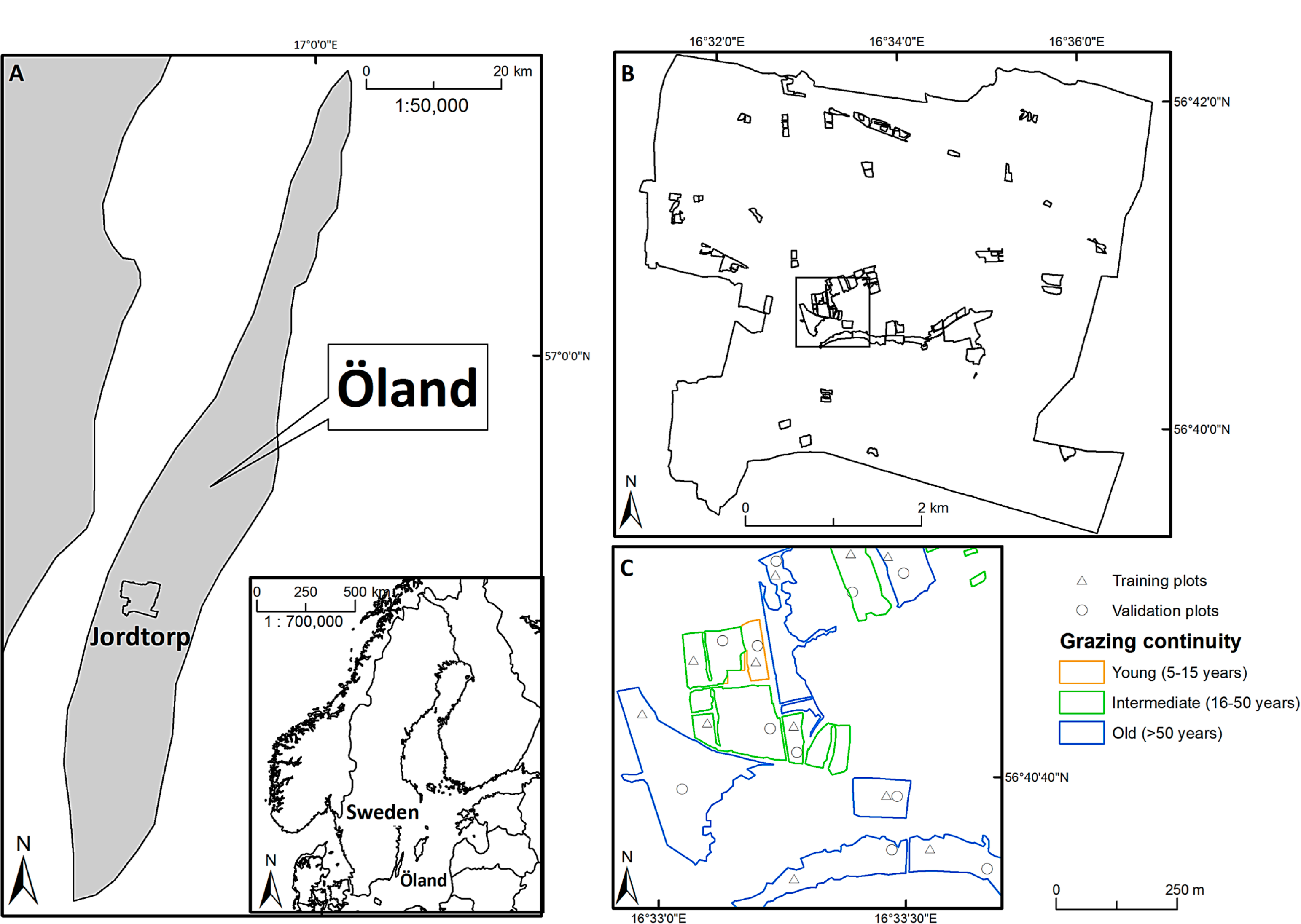
The study area (centred on 56°40′49″N, 16°33′58″E) covers approximately 22.5 km2 and is located on the Baltic island of Öland in SE Sweden (Figure 1A). The bedrock consists of Cambro-Silurian limestone, the average elevation is approximately 36 m above sea level, and the overall topography is flat [48]. The area is crossed by a few low ridges of glaciofluvial deposits. The mean annual temperature is 7 °C and the mean annual precipitation is 468 mm [48]. The present-day landscape consists of a mosaic of arable fields, villages, forests, and grasslands. The majority of the grasslands are grazed, with varying intensity, mainly by cattle.
Detailed information on the historical land use within the study area is available [49]. Whereas the study area was dominated by grasslands during the 18th century [49], most (>80%) of the ancient grasslands have been transformed to arable land during the last 300 years [49]. Approximately 15% of the current grasslands have developed during the last 50 years on previously arable land [49].
2.2. Grassland Sites and Grassland Age-Classes
Using historical and present-day land-use maps, aerial photographs [49] and field inventories, we identified 299 grazed grassland sites that were separated from each other and the surrounding landscape by walls or fences. With the help of geographic information system (GIS) overlay analysis of the land-use maps and aerial photographs, the sites were categorized according to their grazing continuity (grassland age) and assigned to one of three age-classes within the arable-to-grassland succession; 5–15 (young grasslands), 16–50 (intermediate-aged grasslands), and >50 (old grasslands) years of grassland continuity (Figure A1).
Within each site, two sampling points were randomly positioned in open (not covered by shrubs or trees) grassland vegetation, with the constraints that they should be at least 25 m apart (to minimize effects of spatial autocorrelation in the vegetation), at least 13.5 m from the site boundary (to minimize edge-effects in the vegetation [50]), and at least 13.5 m from shrubs or trees higher than 50 cm (to minimize shading-effects). In total 239 grassland sites (89 young, 73 intermediate, and 77 old) out of the 299 sites could accommodate these constraints. From these 239 grassland sites, we randomly selected 60 sites (20 young, 20 intermediate, and 20 old). Within these 60 sites, a bioassay approach (cf. [51,52]) based on indicator species (such as Sesleria caerulea and Molinia caerulea) was used to define sites with “dry” grassland vegetation, and exclude moister grassland vegetation. A total of 52 sites (17 young, 18 intermediate, and 17 old) out of the 60 sites were characterized by dry grassland vegetation and used for the vegetation and remote sensing sampling (Figure 1B). Of the 17 “old” sites, 13 sites had a management continuity of >280 years [49]: the vegetation in these sites falls within the Natura 2000 habitat type “Fennoscandian lowland species-rich dry to mesic grasslands”.
A hand-held differential global positioning system (DGPS) receiver (Topcon GRS-1 GNSS, equipped with a PG-A1 external antenna (Topcon Corporation, Japan)) connected to a real-time positioning service (SWEPOS) was used to log (with an accuracy of ∼1 cm) the ground coordinates of the two sampling points within each of the 52 grassland sites. The sampling points were divided into two data sets (a training and a validation data set) by randomly assigning the two sampling points from each site to one or other of the two data sets (Figure 1C).
2.3. Plant Community Characteristics
Vegetation sampling was carried out between 15 May and 15 July 2011. A 1 m × 1 m plot was centred over each of the two sampling points within each of the 52 sites. Each of the 104 (1 m × 1 m) plots was divided into a grid of 100 (10 cm × 10 cm) sub-plots, and the presence of all non-woody vascular plants was recorded within each sub-plot (Table A1). For each 1 m × 1 m plot, the frequency of each species was calculated as the number of sub-plots in which the species was present.
The plant species recorded in the 1 m × 1 m plots were assigned values for SLA and two Ellenberg indicator values (for nutrients and moisture availability). The trait information was compiled from the LEDA trait database [53], which provides species-level SLA values that represent aggregated trait values. The LEDA values are based on multiple individuals per species, measured under different environmental conditions. Trait data were not available for the full set of species (n = 185) in the present study. For SLA, previous grassland studies have shown that imputation methods based on multiple imputation by chained equations may be used for filling gaps in functional trait databases [54]. Following Taugourdeau et al. [54], estimates for missing values (approximately 9% of the species) were obtained using the multivariate imputation by chained equation (MICE) method [33,55,56]. Ellenberg indicator values were extracted from the JUICE database [57]: values for the four species that were not found in the database were extracted from Ellenberg et al. [58]. A frequency-weighted mean value (CWM) [35] was calculated, for SLA and each of the Ellenberg values, for each plant community: CWM(x) = ∑ipi × xi, where pi is the relative frequency of the ith species and xi is the trait or Ellenberg index value of the iith species.
The percentage ground cover of grasses was estimated within four 50 cm × 50 cm sub-plots within each 1 m × 1 m plot, and a mean within-plot value for grass cover (excluding dead litter) was calculated for each plot.
2.4. Remote Sensing Data
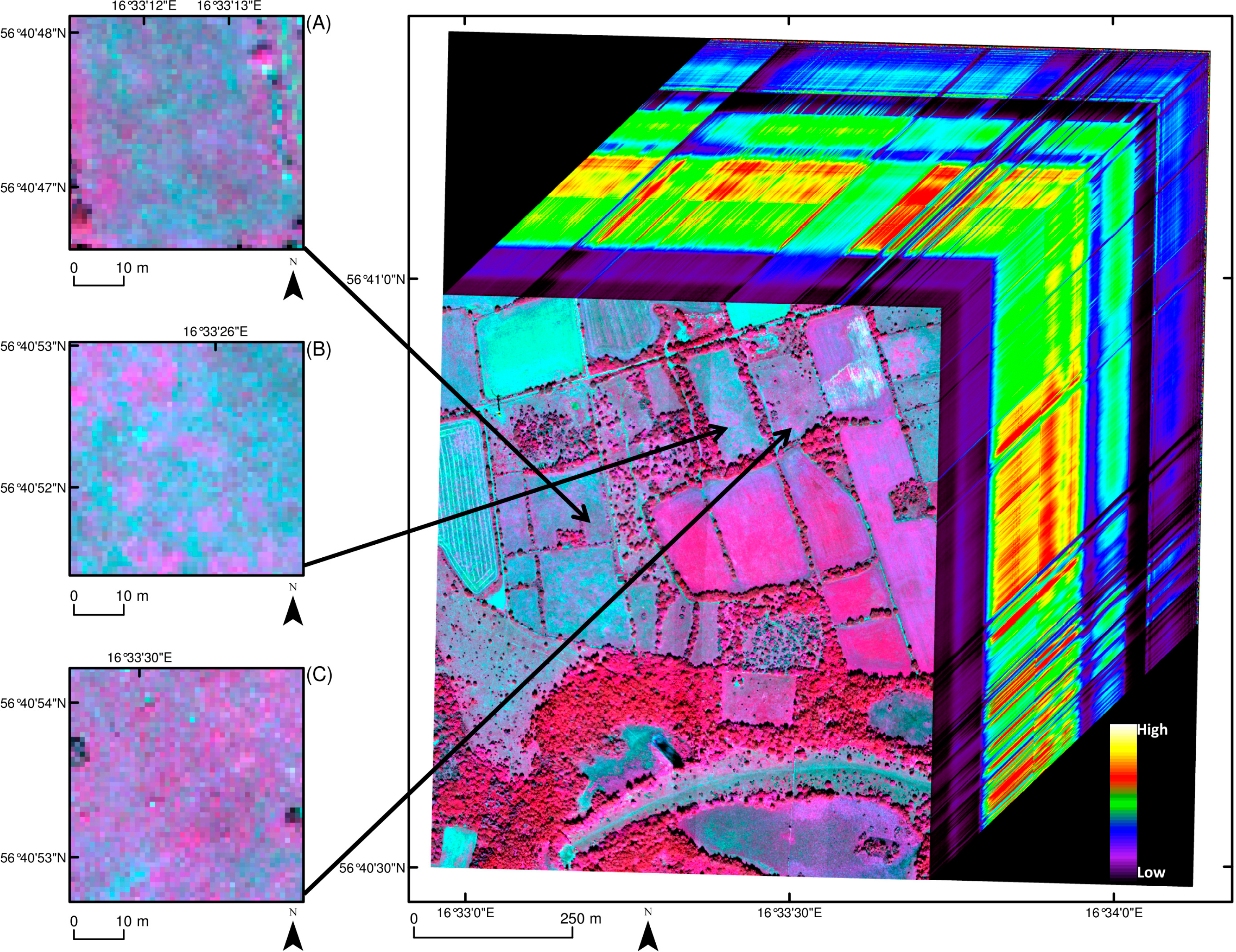
Remote sensing data over the study area were acquired on 9 July 2011. Twenty-five flight lines were recorded at around solar noon, using two airborne HySpex hyperspectral spectrometers (Norsk Elektro Optikk AS (NEO), Lörenskog, Norway), and a push-broom scanning mode at a flight altitude of approximately 1500 m. The flight was carried out by Terratec AS, Lysaker, Norway. All flight lines were conducted either from north to south or from south to north to minimize illumination effects. The output from the two HySpex spectrometers (VNIR-1600 operating over the 414 to 991 nm range and SWIR-320m-e operating over the 966 to 2501 nm range) consisted of 416 wavebands with spectral resolutions of 3.7 nm (VNIR-1600) and 6.0 nm (SWIR-320m-e) (Figure 2). The spatial resolution (pixel size) of the image captured from the VNIR-1600 spectrometer was 0.5 m × 0.5 m and the spatial resolution of the SWIR-320m-e image was 1.0 m × 1.0 m. A digital elevation model (DEM) was created with the help of LiDAR data recorded during the flight.
2.4.1. Pre-Processing of HySpex Data
Physically based atmospheric correction of the HySpex data was carried out with the help of the ATCOR-4 software [59], which is based on the radiative transfer model MODTRAN 5 [60]. In accordance with the standard procedure in the ATCOR-4 software, the following atmospheric parameters were used during the correction process: desert aerosol model, water vapour column of 1.0 g·m−2, visibility of 28.4 km, and an ozone concentration of 330 Dopson units. The conversion of radiance into reflectance was based on the Fontenla-2011 solar irradiance spectrum [61,62]. While the overall topography within the study area is flat, there are local differences in elevation. To account for surface elevation, slope, and orientation, the correction for topographic illumination effects was carried out in the “rugged terrain” model of the ATCOR-4 software using the DEM created with the help of the LiDAR data recorded during the flight. The spectral data acquired with the help of the VNIR-1600 spectrometer were resampled to a spatial resolution of 1 m × 1 m (with the help of a triangulated nearest neighbourhood method) and to a spectral resolution of 6.0 nm (by LOESS interpolation) to match the data collected from the SWIR-320m-e spectrometer. A Savitzky-Golay smoothing filter [63], with a degree of 3 and a width of 9 was used to reduce the effect of random noise in the spectral data. Following [64], brightness normalization was carried out to dampen differences in the brightness of the spectra caused by subpixel shade. The interpolation was done using the hyperSpec package [65] and the filtering was done using the signal package [66] in the R statistical environment [67]. The images were orthorectified by the HySpex data providers (Terratec AS, Lysaker, Norway) using the PARGE software [60] to a spatial accuracy of approximately 0.3 m for both the VNIR-1600 and SWIR-320m-e spectral bands.
2.4.2. Extracting HySpex Data
Spectral bands that (i) overlapped between the two spectrometers (962–985 nm) and (ii) were in spectral domains that are strongly influenced by atmospheric water vapour absorption (1321–1443 nm, 1803–2032 nm and 2420–2501 nm) were deleted (cf. [68,69]). A pixel window of 3 × 3 pixels (3 m × 3 m) for the remaining 269 bands (414–2417 nm) was centred on each of the 52 coordinate points associated with the training and validation data sets. The mean spectral value for each of the 269 HySpex bands was calculated for the pixels falling within each of the 104 pixel windows.
2.5. Statistical Analyses
2.5.1. Partial Least Squares Discriminant Analysis
PLS regression [43] allows statistical analysis of data sets where the explanatory variables are strongly correlated and where the number of explanatory variables is similar to or higher than the number of samples [70,71]. Whereas the use of a high number of inter-correlated explanatory variables may influence random noise, which, in its turn, may lead to model overfitting and reduced model accuracy, PLS regression builds on the assumption that only a few variables influence the process that is under study. By combining the information in a large number of inter-correlated explanatory variables into a few latent components, the risk of model overfitting is reduced in PLS [72]. The latent variables (LVs) are identified by finding the loading weights for each explanatory variable that maximize the covariance between the explanatory variables and the dependent variables. In the case of binary dependent variables, the PLS algorithm [43] can be used for discriminatory purposes [73].
A PLS-DA based on hyperspectral data and vegetation data was carried out to assess whether (i) the three grassland age-classes can be classified with the help of HySpex data, and (ii) it is possible to identify a subset of HySpex wavebands that can be used for the classification of the grassland age-classes. Two PLS-DA models—Model 1 developed from the full set of HySpex bands and Model 2 from a subset of HySpex bands—were generated and the capabilities of the two models for classifying grassland age-classes were compared.
The two models were developed using a similar PLS-DA-based procedure. Initially, a binary membership vector was built for each grassland age-class individually. For each of the three individual grassland age-class membership vectors, each individual plot was defined as 1 (belonging to a particular age-class) or 0 (not belonging to a particular age-class). The three membership vectors were used to build the dependent matrix. The explanatory matrix was generated from the HySpex bands representing the plots associated with the training data set (n = 52). An increasing number of latent variables will normally improve the predictive capability of a PLS-DA model because several variables can carry more information than a few [74]. However, because too many latent variables can overfit the final model, the optimal number of latent variables needs to be identified (cf. [75]). In the present study, the number of latent variables that gave the lowest misclassification rate was used in the final model.
The training data sets associated with the two models were used to quantify their accuracies for classifying grassland age-classes with the help of tenfold cross-validated discriminant analysis. The validation data sets associated with the models were used to evaluate them for the training data sets by fitting the final cross-validated PLS-DA models of the training data sets to the validation data sets. The calculations were implemented in the R statistical environment [67] using the pls package [76].
2.5.2. Explanatory Matrices Used in the Two PLS-DA Models
The explanatory matrix used for Model 1 included 269 spectral bands. The relative importance of each individual predictor variable (i.e., each HySpex band) in Model 1 was described by the variable importance in projection (VIP) value [77]. The HySpex bands associated with VIP values greater than 0.8 (cf. [78]) in Model 1 were assigned to a subset of spectral bands. The explanatory matrix used for Model 2 was then based on the subset of HySpex bands.
2.5.3. Accuracies of the PLS-DA Models Used for the Classification of Grassland Age-Classes
Two approaches were used to quantify the ability of each of the two PLS-DA models to classify grassland age-classes:
- (i)
Tenfold cross-validation was used on the training data set and a confusion matrix was created to assess the accuracy of the HySpex based classification of the three grassland age-classes. With the help of the confusion matrix, the producer’s accuracy and the user’s accuracy were calculated for each age-class. The producer’s accuracy refers to the probability that a plot associated with a specific grassland age-class on the ground will be assigned to the correct age-class on the basis of the grassland spectral response acquired from the plot. The user’s accuracy represents the probability that a grassland plot classified (with the help of the grassland spectral response acquired from the plot) as belonging to a specific grassland age-class is associated with this class on the ground. The overall prediction accuracy and the Kappa statistic value [79,80], which assesses the interclassifier agreement, were also calculated from the confusion matrix.
- (ii)
The final cross-validated model of the training data set was fitted to the validation data set and used to classify the age-class of each plot associated with the validation data set. The predictive capability of the PLS-DA model was investigated by calculating the producer’s and user’s accuracy for each age-class associated with the validation data set. The overall prediction accuracy and Kappa statistic value [79,80] for the classification results based on the validation data set were also calculated.
3. Results
3.1. Classification Based on the Full Set of 269 HySpex Wavebands (Model 1)
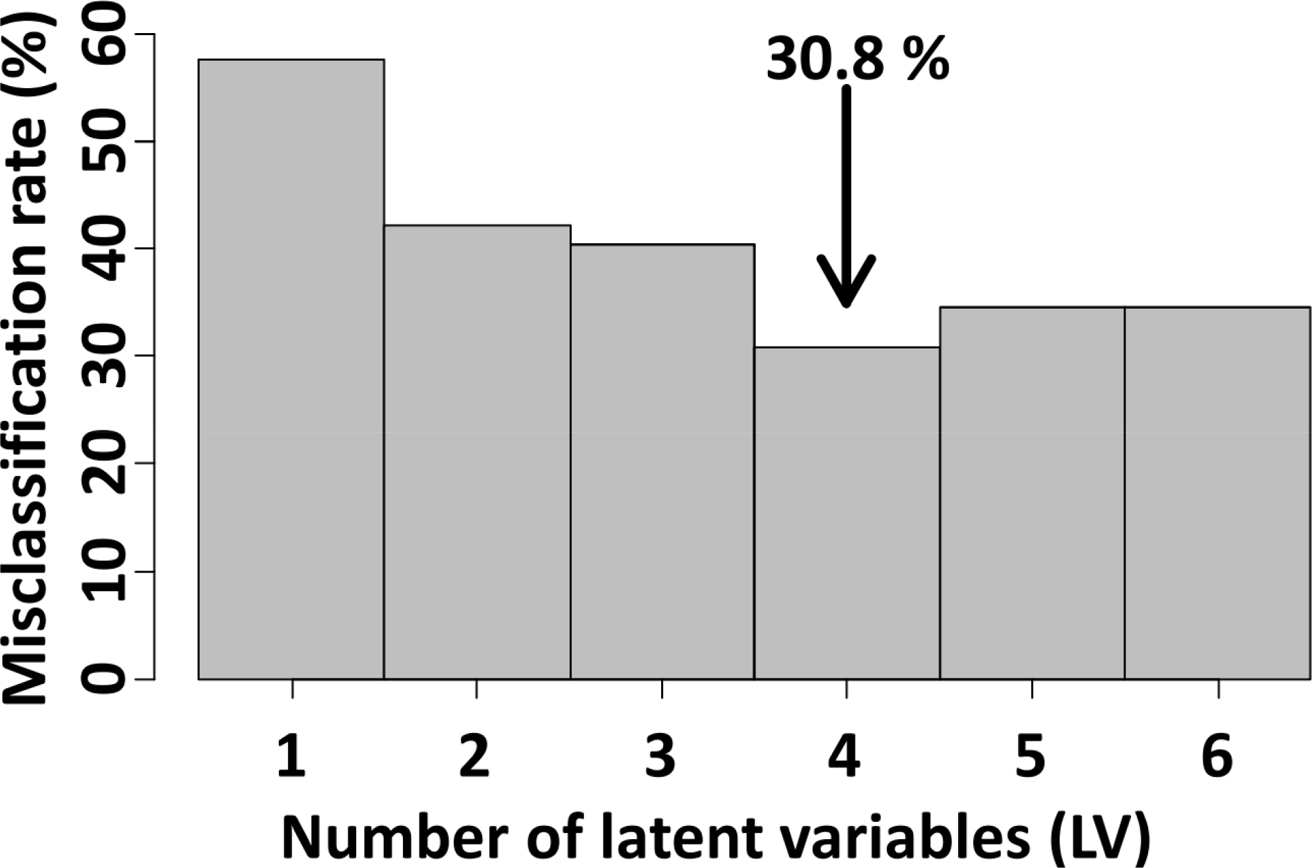
The misclassification rate decreased progressively with the number of latent variables (from 57.7% with one latent variable), reaching a minimum (30.8%; Figure 3) with the first four latent variables before increasing again. We used the first four latent variables in the final model.
The producer’s and user’s classification accuracies for the individual grassland age-classes varied between 47% and 100% for the training data set, and between 65% and 94% for the validation data set (Table 1).
The overall classification accuracy and the Kappa statistic value were 77% and 0.65, respectively, for both the training and the validation data set (Table 1).
3.2. The HySpex Wavebands That are Most Important for the Classification of Grassland Age-Classes
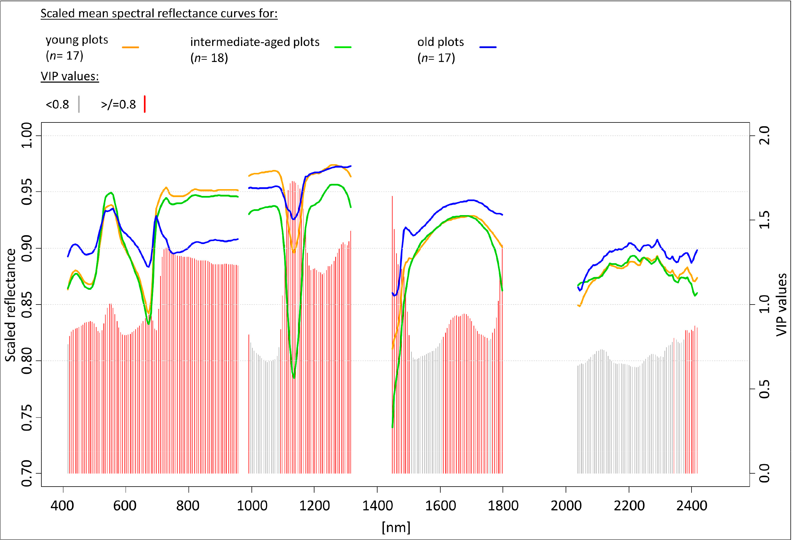
The VIP value is an indicator of the relative influence of each predictor in a PLS model. Out of the 269 HySpex bands used as explanatory variables in the PLS-DA model, 177 bands had VIP values greater than 0.8, indicating that these bands were the most important predictor variables in the remote sensing-based classification of grassland age-classes (Figure 4). In total, 14 wavebands in the blue region (414–499 nm), 16 wavebands in the green region (505–596 nm), 20 wavebands in the red region (602–716 nm), 17 wavebands in the red-edge portion (722–818 nm), 23 wavebands in the NIR1 part (824–969 nm), 39 wavebands in NIR2 part (975–1394 nm), and 48 wavebands in the SWIR portion (1448–2417 nm) of the electromagnetic spectrum were associated with VIP scores greater than 0.8 (Figure 4).
3.3. Classification Based on a Reduced Set of HySpex Wavebands (Model 2)
The subset of HySpex bands used to develop Model 2 included the 177 spectral bands that were associated with VIP values greater than 0.8 in the model based on the full set of 269 HySpex bands. The inclusion of four latent variables gave the lowest misclassification rate in the second PLS-DA model.
The producer’s and user’s classification accuracies for the individual grassland age-classes for Model 2 varied between 65% and 94% for the training data set (Table 2). The classification accuracies for the individual grassland age-classes for the validation data set ranged between 74% and 94% (Table 2). The overall classification accuracy and the Kappa statistic value were 81% and 0.71, respectively, for the training data set and 85% and 0.77, respectively, for the validation data set (Table 2).
For the validation data sets, the overall classification accuracy and the Kappa statistic value were higher for Model 2 than for Model 1 (Tables 1 and 2). The differences in classification accuracies between the two models were 8% for the overall accuracy and 0.12 for the Kappa statistic value (Tables 1 and 2).
3.4. Plant Community and Spectral Characteristics of Grasslands Representing Different Age-Classes
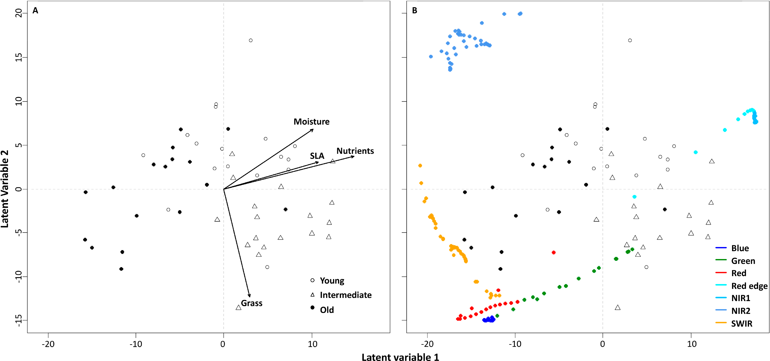
The first four latent variables (LV1–LV4) in Model 2 explained 34%, 41%, 12%, and 10% of the variation in the explanatory matrix (spectral data), respectively. Old (negative scores) and intermediate-aged (positive scores) grassland plots were separated on the first latent variable (LV1), whereas LV2 discriminated between young (positive scores) and intermediate-aged (negative scores) plots (Figure 5A).
Correlation coefficients between the scores for grassland plots on the first two latent variables, and the ecological variables (SLA, Ellenberg indicator value for nutrients and moisture availability, and the percentage cover of grasses) were calculated with the help of multiple regressions. Significance values for the correlation coefficients were based on 9999 permutations. The correlation coefficients are represented as arrows in Figure 5A, with the direction and length of the arrow indicating, respectively, the sign and the strength of the correlation coefficient. The scores for the grassland plots were significantly associated with the mean within-plot Ellenberg indicator values for nutrient availability (p = 0.010), and with the within-plot cover of grasses (p = 0.045). The young plots were characterized by the highest and the old plots by the lowest indicator values for nutrients, whereas the intermediate-aged plots were characterized by the highest cover of grasses (Figure 5A). The mean within-plot SLA and Ellenberg indicator value for moisture were not significantly associated with the plot scores in the PLS-DA.
The old plots were associated with negative loadings for the blue, red, and SWIR regions on the first latent variable, and the intermediate-aged plots were associated with positive loadings for the red-edge and NIR1 regions (Figure 5B). The old plots, which are characterized by lower indicator values for nutrients than the intermediate-aged plots (Figure 5A), had higher reflectance values than the intermediate-aged plots in the blue, red, and SWIR regions. The intermediate-aged plots, which are characterized by higher cover of grasses than the old plots (Figure 5A), had higher reflectance values than the old plots in the green, red-edge, and NIR1 regions (Figure 5B).
On LV2, the young plots were associated with positive loadings for the red-edge, NIR1, and NIR2 regions, while the intermediate-aged plots were associated with negative loading for the green region (Figure 5B). The young plots, which are characterized by higher indicator values for nutrients than the intermediate-aged plots (Figure 5A), had higher reflectance values than the intermediate-aged plots in the red-edge, NIR1, and NIR2 regions (Figure 5B). The intermediate-aged plots, which are characterized by higher cover of grasses than the young plots (Figure 5A), had higher reflectance than the young plots in the green region (Figure 5B).
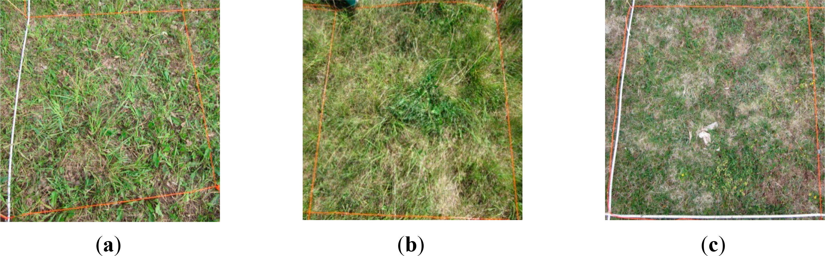
Species lists for each of the three grassland age-classes are provided in Table A1 (Supporting information). Figure A1 (Supporting information) shows a field photograph of a sample plot representing each of the three grassland age-classes.
4. Discussion
4.1. PLS-DA Based Classification of Grassland Age-Classes
The three age-classes in our study were successfully classified using a pre-selected set of hyperspectral wavebands and PLS-DA, indicating that fine-scale hyperspectral measurements are able to accurately identify grassland successional stages within a local landscape. Our results are consistent with those of earlier studies of other types of vegetation that also show that the exclusion of wavebands that provide little information related to the response variable improves the PLS-DA based classification of plant communities [47,81]. For example, using airborne AISA Eagle hyperspectral imagery, Peerbhay et al. [47] showed that a PLS-DA model based on the 78 wavebands that were most relevant for the classification of forest species gave 8.17% higher overall classification accuracy than a model utilising all 230 AISA Eagle wavebands. Our results are also consistent with the results of Peerbhay et al. [47] in that they show that a high number of hyperspectral wavebands can be compressed into a few latent variables with the help of PLS, reducing the risk of model overfitting and, at the same time providing a successful classification of different vegetation types.
4.2. Spectral Dissimilarities between Grasslands Belonging to Different Age-Classes
The majority of the present-day grazed grasslands in Sweden originate from abandoned arable fields that have been cultivated as leys [82] and seeded with grasses, such as Lolium perenne, Festuca pratensis, Poa pratensis, and Phleum pratense (cf. [83]). The effects of the addition of nutrients during arable cultivation may persist during the early stages of the arable-to-grassland succession [84,85]. Recently cultivated fields, such as the young grasslands in our study (Figure 5A), are generally characterized by a high availability of nutrients that allows nitrophilous and ruderal species (fast growing and disturbance-tolerant species) to invade and restricts the establishment of less competitive species during early succession (cf. [33]). Early-successional grasslands are typically characterized by species that are adapted to nutrient-rich environments (e.g., Dactylis glomerata, Poa pratensis, and Geranium molle [86]) and nutrient-rich vegetation commonly contains plants with a relatively high SLA [87]. An increased availability of nutrients may result in greater above-ground production of biomass (cf. [85]), which, in its turn, influences the light conditions within the vegetation canopy: an increased leaf area represents a common adaptation to low light environments [38,88].
Residual effects of fertilization during arable cultivation may still persist within the intermediate-aged grasslands in our study (cf. [84,85]). However, the fact that continuous grazing management contributes to the removal of nutrients explains the reduced abundance of nitrophilous species during the second successional time step. Previous investigations within the study area have shown that grasslands with a grazing continuity of 16–50 years (corresponding to the intermediate-aged grasslands in the present study) are characterized by significantly lower community mean values for SLA than grasslands that have been grazed for 5–15 years (corresponding to the young grasslands in the present study) [33].
During the third successional time step, a long continuity of grazing management has contributed to a substantial reduction of nutrient levels, allowing species with a low competitive ability to establish in the old grasslands. Purschke et al. [33] showed that, within the study area, values of community-level SLA are lower in grassland sites that have been grazed for more than 51 years (corresponding to the old grasslands in the present study) than in sites with a shorter grazing continuity. Long grazing continuity is essential for the maintenance and establishment of species-rich ancient grassland vegetation characterized by, for example, Festuca ovina and Helianthemum nummularium [89].
Changes in habitat conditions during the arable-to-grassland succession have been shown to be accompanied by changes in plant functional composition and vegetation properties within the same study area [33,90]. In addition, changes in, for example, leaf nitrogen content, SLA, leaf chlorophyll content, leaf water content, and above-ground biomass have shown to be followed by changes in the vegetation spectral response within a range of different habitats [26,91–93]. For example, previous remote sensing studies have revealed that differences in leaf nitrogen content have strong influence on the reflectance from vegetation across the electromagnetic spectrum (visible (400–700 nm) [94], NIR (700–1300 nm) [95], SWIR (1300–2500 nm) [96]). The red-edge region has, been used to estimate the nitrogen concentration in ryegrass (Lolium spp.) [97], and SLA has previously been shown to influence reflectance in several wavebands. For example, Lymburner et al. [98] estimated SLA at the landscape scale with the help of broadband satellite data, and Asner et al. [99] showed that hyperspectral measurements were related to the SLA of tropical forest leaves. The SWIR wavelengths have been shown to be most important for estimation of leaf mass per area (the inverse of SLA [100]).
In the present study, differences in ecological variables (availability of nutrients and cover of grasses) between grassland age-classes are associated with differences in the spectral response from the grasslands (Figure 5). The low blue (414–499 nm) as well as the red (602–716 nm) and the high red-edge (722–818 nm) reflectance for the young plots (Figure 5B) suggest that these plots have a higher chlorophyll content in the vegetation than the old plots. Earlier remote sensing studies have shown that the chlorophyll content in grasslands can be assessed at both fine and landscape scales [46,101], and Darvishzadeh et al. [46] used the red-edge region to map canopy chlorophyll content in heterogeneous grasslands.
The higher cover of grasses (excluding dead litter) in the intermediate-aged plots compared with the young and old plots can be expected to lead to higher green (505–596 nm) reflectance in the intermediate-aged plots. Spectral measurements near the green reflectance peak at 550 nm have previously been shown to be important for the classification of vegetation communities (e.g., [47]).
The high red-edge (722–818 nm) and NIR1 (824–969 nm) reflectance for the young and intermediate-aged plots suggest that these plots were associated with larger above-ground biomass than the old plots (cf. [45]). The low NIR2 (975–1394 nm) reflectance for the intermediate-aged and the low SWIR (1448–2417 nm) reflectance for the young plots indicate that these were characterized by higher canopy moisture than the old plots. The SWIR wavelengths are strongly affected by water absorption [100]; in particular, the moisture-sensitive bands around 1200 nm (located in the NIR2 region in the present study) have been shown to be sensitive to the water content of vegetation in mixed woodland [102] and in grasslands [68].
Trampling by grazing animals is likely to lead to differences in the cover of bare soil between the different age-classes. Spectral dissimilarities between the grasslands belonging to different successional stages may also be explained by between-site edaphic dissimilarity (cf. [103]). The red part of the visible electromagnetic spectrum has been shown to be highly influenced by variation in soil properties [104]. Furthermore, increased levels of shading are expected within the vegetation cover as the above-ground biomass increases. Increased amounts of shadow are accompanied by a decrease in reflectance in all wavebands [105]. The presence of shadows may also have contributed to between-stage spectral dissimilarities in the present study. Monocotyledonous plants, such as grasses, have a compact leaf mesophyll structure, and a lower reflectance in the NIR than plants with a more porous mesophyll structure [106]. The high cover of grasses within the intermediate-aged grasslands in our study may have contributed to between-grassland stage spectral differences in the NIR. Grazing management decreases the accumulation of dead above-ground biomass [107] and the amount of litter has shown to affect the spectral response of grassland vegetation [108]. Our different-aged grassland plots—characterized by different continuity of grazing—may be expected to be associated with different amount of litter, which, in its turn, may have contributed to the spectral dissimilarities between the plots.
The results of our study are consistent with the results from previous ecological studies, which show that plant community characteristics such as the cover of grasses and community-weighted mean Ellenberg indicator values for nutrient availability, change during grassland succession [34,109]. The results of the present study also agree with those of previous interdisciplinary studies within remote sensing and ecology. Earlier studies have shown, for example, that hyperspectral reflectance measurements in grasslands are related to community-weighted mean Ellenberg indicator values for nutrient availability and for plant functional traits, such as SLA [12,32,93].
Although the accuracy of the predictions we obtained using models 1 and 2 were high, some grassland plots in our sample study were not classified correctly by either model. There are a number of possible reasons for this discrepancy. First, we conducted the spectral measurements in early July, when leaf senescence in response to summer drought is likely to have reduced the spectral differences between grassland age-classes. Second, hyperspectral images are known to be affected by radiometric noise [110]. While we used the commonly applied Savitzky-Golay filter [63], other denoising methods, such as the Minimum Noise Fraction (MNF) transform [111], might have improved the noise-reduction in our data. Thirdly, PLS-DA may not be the most optimal method for classifying grassland age-classes. Other classification methods, such as artificial neural networks or support-vector machines (cf. [112]), which are able to take into account non-linear relationships between dependent and explanatory variables, might provide better discrimination between grassland successional stages.
4.3. Future Directions
Future research targeting the improvement of hyperspectral methods for classifying grassland successional stages may include the development of vegetation spectral indices (e.g., [93]), which could potentially provide enhanced information on the plant community characteristics associated with different grassland successional stages. There is also a need for studies that focus on the development of classification methods for discriminating between age-classes at the scale of entire grassland sites. In addition, in order to be able to develop the possible use of hyperspectral data as a source of information within ecological research, we need a better understanding of the ways in which different plant community variables (characterizing different grassland successional stages) influence the hyperspectral response. The spectral response of vegetation canopies changes over the vegetation period as a result of temporal variation in the biochemical and structural properties that influence the reflectance of the vegetation canopy [44]. Additional studies will need to explore seasonal variation in the relationships between hyperspectral data and plant community variables.
5. Conclusions
In the present study we demonstrate that remote sensing data, acquired with the help of two airborne HySpex hyperspectral spectrometers (together covering 414 to 2501 nm), can be used to discriminate between dry grassland vegetation associated with different stages of arable-to-grassland succession within a local agricultural landscape in Sweden. Differences between the spectral responses of different grassland successional stages were associated with differences in the Ellenberg indicator value for nutrient availability and in the ground-cover of grasses.
We analysed the hyperspectral data using partial least squares discriminant analysis—a recently introduced method for the remote sensing-based classification of vegetation (e.g., [47])—and successfully classified grasslands into three different grassland age-classes, representing 5–15, 16–50, and >50 years of grazing management, respectively. We used an independent validation dataset to evaluate the classification-accuracy of our method.
The study shows that the variable importance in projection method [77] can be used to identify the wavebands that are the most important predictor variables in the hyperspectral classification of grassland age-classes. The accuracy of a partial least squares classification based on a subset of 177 wavebands, identified with the help of the variable importance in projection approach as those that were most important for discriminating between successional stages, was 85% (8% higher than for a classification based on the full set of 269 bands). Among the 177 hyperspectral wavebands that gave the most efficient discrimination between grassland age-classes, 50 wavebands were located in the visible region (414–716 nm), 79 wavebands in the red-edge to near-infrared regions (722–1394 nm), and 48 wavebands in the shortwave infrared region (1448–2417 nm) of the electromagnetic spectrum. The fact that the best wavebands for discriminating between grassland age-classes fell within the operating range of both the HySpex VNIR-1600 spectrometer (414 to 991 nm) and the HySpex SWIR-320m-e spectrometer (966 to 2501 nm) suggests that data from specific wavebands covering the full 400–2500 nm spectral range are likely to provide the best classification of grassland successional stages. Our results also show that the partial least squares-based classification procedure is a suitable method for the classification of grasslands successional stages, allowing a large number of hyperspectral wavebands to be compressed into a few latent variables while decreasing the risk of model overfitting. In our study, the first four latent variables explained approximately 97% of the variation in the spectral data.
A recent horizon-scan review [16] identifies 15 issues, or emerging topics, that are expected to have increasingly important implications for the global conservation of biological diversity, and which require wider consideration. The potential use of remote sensing-based techniques for monitoring land cover change is recognized as one of the 15 topics, and the review identifies the need to develop remote sensing methods for monitoring land cover change at detailed spatial scales and over large areas. Native grasslands are specifically mentioned as a type of land cover that is currently relatively difficult to monitor with the help of remote sensing techniques [16]. The results of the present study demonstrate that airborne hyperspectral data are capable of capturing detailed-scale information that discriminates between grassland plant communities representing different stages of an arable-to-grassland succession within a local landscape—suggesting that a similar approach may hold promise for the remote sensing-based mapping of grasslands belonging to different successional stages over larger areas.
There are a number of possible ways in which the methodology that we used might be improved in future studies. For example, whereas the present study was based on remote sensing data from a single time-point, a multi-temporal approach is likely to improve the ability to discriminate successfully between grasslands belonging to different successional stages. Future studies should use spectral data collected at different time-points during the vegetation season. In our study, we only used one method (the Savitzky-Golay filter) to reduce radiometric noise in the hyperspectral data: subsequent studies should explore the relative efficiencies of different denoising methods. Finally, because aerial remote sensing systems have a smaller coverage area than satellite-based remote sensing systems, future studies should investigate the possibility of using hyperspectral satellite data, for example data acquired with the help of the Hyperion satellite [113] and the planned EnMAP satellite [114], for monitoring grassland successional stages over wider areas in agricultural landscapes.
Abbreviations
| ATCOR | Atmospheric and Topographic Correction |
| CWM | Community-Weighted Mean |
| DEM | Digital Elevation Model |
| DGPS | Differential Global Positioning System |
| GIS | Geographic Information System |
| LDMC | Leaf Dry Matter Content |
| LiDAR | Light Detection and Ranging |
| LMA | Leaf Mass per Area |
| LOESS | Local Polynomial Regression |
| LV | Latent Variable |
| MICE | Multivariate Imputation by Chained Equations |
| MODTRAN | Moderate Resolution Atmospheric Transmission |
| NEO | Norsk Elektro Optikk |
| NIR | Near-Infrared |
| PARGE | Parametric Geocoding |
| PLS | Partial Least Squares |
| PLS-DA | Partial-Least-Squares Discriminant Analysis |
| SLA | Specific Leaf Area |
| SWIR | Short-Wave Infrared |
| VIP | Variable Importance in Projection |
| VNIR | Visible and Near Infrared |
Acknowledgments
The study was financed by grants from The Swedish Research Council for Environment, Agricultural Sciences and Spatial Planning (FORMAS) to Karin Hall and Honor C. Prentice. We thank Sofia Pallander, Andreas Press, and Johan Rydlöv for field assistance. The “Station Linné” research station at Ölands Skogsby was used as a base for the fieldwork. We are grateful to the anonymous reviewers for their valuable comments on an earlier version of the manuscript. The study is a contribution to the Lund University Strategic Research Area “Biodiversity and Ecosystem Services in a Changing Climate” (BECC). Oliver Purschke acknowledges the support of the German Centre for Integrative Biodiversity Research (iDiv) Halle-Jena-Leipzig, funded by the German Research Foundation (FZT 118).
Author Contributions
Thomas Möckel, Jonas Dalmayne, Honor C. Prentice and Karin Hall planned and participated in the field work. Thomas Möckel, Jonas Dalmayne and Karin Hall planned the collection of remotely sensed data. Thomas Möckel processed and analysed the data. All authors were involved in the research design, the interpretation of results, and the preparation of the manuscript.
Conflicts of Interest
The authors declare no conflict of interest.
References
- Benton, T.G.; Vickery, J.A.; Wilson, J.D. Farmland biodiversity: Is habitat heterogeneity the key? Trends Ecol. Evol 2003, 18, 182–188. [Google Scholar]
- Eriksson, O.; Cousins, S.A.O.; Bruun, H.H. Land-use history and fragmentation of traditionally managed grasslands in Scandinavia. J. Veg. Sci 2002, 13, 743–748. [Google Scholar]
- Tscharntke, T.; Klein, A.M.; Kruess, A.; Steffan-Dewenter, I.; Thies, C. Landscape perspectives on agricultural intensification and biodiversity—Ecosystem service management. Ecol. Lett 2005, 8, 857–874. [Google Scholar]
- Cramer, V.A.; Hobbs, R.J.; Standish, R.J. What’s new about old fields? Land abandonment and ecosystem assembly. Trends Ecol. Evol 2008, 23, 104–112. [Google Scholar]
- Reger, B.; Mattern, T.; Otte, A.; Waldhardt, R. Assessing the spatial distribution of grassland age in a marginal European landscape. J. Environ. Manag 2009, 90, 2900–2909. [Google Scholar]
- Cramer, V.; Hobbs, R.J. Old Fields: Dynamics and Restoration of Abandoned Farmland; International Island Press: Washington, DC, USA, 2007. [Google Scholar]
- Cousins, S.A.O.; Lindborg, R.; Mattsson, S. Land use history and site location are more important for grassland species richness than local soil properties. Nord. J. Bot 2009, 27, 483–489. [Google Scholar]
- Lengyel, S.; Varga, K.; Kosztyi, B.; Lontay, L.; Déri, E.; Török, P.; Tóthmérész, B. Grassland restoration to conserve landscape-level biodiversity: A synthesis of early results from a large-scale project. Appl. Veg. Sci 2012, 15, 264–276. [Google Scholar]
- Stevenson, M.J.; Bullock, J.M.; Ward, L.K. Re-creating semi-natural communities: Effect of sowing rate on establishment of calcareous grassland. Restor. Ecol 1995, 3, 279–289. [Google Scholar]
- Purschke, O.; Sykes, M.T.; Reitalu, T.; Poschlod, P.; Prentice, H.C. Linking landscape history and dispersal traits in grassland plant communities. Oecologia 2012, 168, 773–783. [Google Scholar]
- Kerr, J.T.; Ostrovsky, M. From space to species: Ecological applications for remote sensing. Trends Ecol. Evol 2003, 18, 299–305. [Google Scholar]
- Schmidtlein, S. Imaging spectroscopy as a tool for mapping Ellenberg indicator values. J. Appl. Ecol 2005, 42, 966–974. [Google Scholar]
- Rocchini, D.; Balkenhol, N.; Carter, G.A.; Foody, G.M.; Gillespie, T.W.; He, K.S.; Kark, S.; Levin, N.; Lucas, K.; Luoto, M.; et al. Remotely sensed spectral heterogeneity as a proxy of species diversity: Recent advances and open challenges. Ecol. Inform 2010, 5, 318–329. [Google Scholar]
- Gillespie, T.W.; Foody, G.M.; Rocchini, D.; Giorgi, A.P.; Saatchi, S. Measuring and modelling biodiversity from space. Prog. Phys. Geogr 2008, 32, 203–221. [Google Scholar]
- Ustin, S.L.; Gamon, J.A. Remote sensing of plant functional types. New Phytol 2010, 186, 795–816. [Google Scholar]
- Sutherland, W.J.; Aveling, R.; Brooks, T.M.; Clout, M.; Dicks, L.V.; Fellman, L.; Fleishman, E.; Gibbons, D.W.; Keim, B.; Lickorish, F.; et al. A horizon scan of global conservation issues for 2014. Trends Ecol. Evol 2014, 29, 15–22. [Google Scholar]
- Waldhardt, R.; Otte, A. Indicators of plant species and community diversity in grasslands. Agric. Ecosyst. Environ 2003, 98, 339–351. [Google Scholar]
- Kawamura, K.; Akiyama, T.; Yokota, H.; Tsutsumi, M.; Yasuda, T.; Watanabe, O.; Wang, S. Quantifying grazing intensities using geographic information systems and satellite remote sensing in the Xilingol steppe region, Inner Mongolia, China. Agric. Ecosyst. Environ 2005, 107, 83–93. [Google Scholar]
- Thenkabail, P.S.; Smith, R.B.; De Pauw, E. Evaluation of narrowband and broadband vegetation indices for determining optimal hyperspectral wavebands for agricultural crop characterization. Photogramm. Eng. Remote Sens 2002, 68, 607–621. [Google Scholar]
- Thenkabail, P.S.; Smith, R.B.; de Pauw, E. Hyperspectral vegetation indices and their relationships with agricultural crop characteristics. Remote Sens. Environ 2000, 71, 158–182. [Google Scholar]
- Chan, J.C.-W.; Paelinckx, D. Evaluation of random forest and adaboost tree-based ensemble classification and spectral band selection for ecotope mapping using airborne hyperspectral imagery. Remote Sens. Environ 2008, 112, 2999–3011. [Google Scholar]
- Thenkabail, P.S.; Enclona, E.A.; Ashton, M.S.; van der Meer, B. Accuracy assessments of hyperspectral waveband performance for vegetation analysis applications. Remote Sens. Environ 2004, 91, 354–376. [Google Scholar]
- Thenkabail, P.S.; Enclona, E.A.; Ashton, M.S.; Legg, C.; de Dieu, M.J. Hyperion IKONOS ALI, and ETM + sensors in the study of African rainforests. Remote Sens. Environ 2004, 90, 23–43. [Google Scholar]
- Jacquemoud, S.; Ustin, S.L.; Verdebout, J.; Schmuck, G.; Andreoli, G.; Hosgood, B. Estimating leaf biochemistry using the PROSPECT leaf optical properties model. Remote Sens. Environ 1996, 56, 194–202. [Google Scholar]
- Curran, P.J. Remote-sensing of foliar chemistry. Remote Sens. Environ 1989, 30, 271–278. [Google Scholar]
- Ustin, S.L.; Gitelson, A.A.; Jacquemoud, S.; Schaepman, M.; Asner, G.P.; Gamon, J.A.; Zarco-Tejada, P. Retrieval of foliar information about plant pigment systems from high resolution spectroscopy. Remote Sens. Environ 2009, 113, 67–77. [Google Scholar]
- Blackburn, G.A. Hyperspectral remote sensing of plant pigments. J. Exp. Bot 2007, 58, 855–867. [Google Scholar]
- Cheng, Y.-B.; Zarco-Tejada, P.J.; Riaño, D.; Rueda, C.A.; Ustin, S.L. Estimating vegetation water content with hyperspectral data for different canopy scenarios: Relationships between AVIRIS and MODIS indexes. Remote Sens. Environ 2006, 105, 354–366. [Google Scholar]
- Darvishzadeh, R.; Skidmore, A.; Atzberger, C.; van Wieren, S. Estimation of vegetation LAI from hyperspectral reflectance data: Effects of soil type and plant architecture. Int. J. Appl. Earth Obs 2008, 10, 358–373. [Google Scholar]
- Ellenberg, H. Zeigerwerte der Gefässpflanzen Mitteleuropas; Goltze: Göttingen, Germany, 1974; Volume 9. [Google Scholar]
- Diekmann, M. Species indicator values as an important tool in applied plant ecology—A review. Basic Appl. Ecol 2003, 4, 493–506. [Google Scholar]
- Klaus, V.H.; Kleinebecker, T.; Boch, S.; Müller, J.; Socher, S.A.; Prati, D.; Fischer, M.; Hölzel, N. NIRS meets Ellenberg’s indicator values: Prediction of moisture and nitrogen values of agricultural grassland vegetation by means of near-infrared spectral characteristics. Ecol. Indic 2012, 14, 82–86. [Google Scholar]
- Purschke, O.; Schmid, B.C.; Sykes, M.T.; Poschlod, P.; Michalski, S.G.; Durka, W.; Kühn, I.; Winter, M.; Prentice, H.C. Contrasting changes in taxonomic, phylogenetic and functional diversity during a long-term succession: Insights into assembly processes. J. Ecol 2013, 101, 857–866. [Google Scholar]
- Pykälä, J.; Luoto, M.; Heikkinen, R.K.; Kontula, T. Plant species richness and persistence of rare plants in abandoned semi-natural grasslands in northern Europe. Basic Appl. Ecol 2005, 6, 25–33. [Google Scholar]
- Garnier, E.; Cortez, J.; Billés, G.; Navas, M.-L.; Roumet, C.; Debussche, M.; Laurent, G.; Blanchard, A.; Aubry, D.; Bellmann, A.; et al. Plant functional markers capture ecosystem properties during secondary succession. Ecology 2004, 85, 2630–2637. [Google Scholar]
- Wright, I.J.; Reich, P.B.; Westoby, M.; Ackerly, D.D.; Baruch, Z.; Bongers, F.; Cavender-Bares, J.; Chapin, T.; Cornelissen, J.H.C.; Diemer, M.; et al. The worldwide leaf economics spectrum. Nature 2004, 428, 821–827. [Google Scholar]
- Shipley, B.; Vu, T.-T. Dry matter content as a measure of dry matter concentration in plants and their parts. New Phytol 2002, 153, 359–364. [Google Scholar]
- Evans, J.R.; Poorter, H. Photosynthetic acclimation of plants to growth irradiance: The relative importance of specific leaf area and nitrogen partitioning in maximizing carbon gain. Plant Cell Environ 2001, 24, 755–767. [Google Scholar]
- Shipley, B. Structured interspecific determinants of specific leaf area in 34 species of herbaceous angiosperms. Funct. Ecol 1995, 9, 312–319. [Google Scholar]
- Viedma, O.; Torres, I.; Pérez, B.; Moreno, J.M. Modeling plant species richness using reflectance and texture data derived from QuickBird in a recently burned area of Central Spain. Remote Sens. Environ 2012, 119, 208–221. [Google Scholar]
- Leutner, B.F.; Reineking, B.; Müller, J.; Bachmann, M.; Beierkuhnlein, C.; Dech, S.; Wegmann, M. Modelling forest alpha-diversity and floristic composition—On the added value of LiDAR plus hyperspectral remote sensing. Remote Sens 2012, 4, 2818–2845. [Google Scholar]
- Pal, M.; Mather, P.M. Support vector machines for classification in remote sensing. Int. J. Remote Sens 2005, 26, 1007–1011. [Google Scholar]
- Wold, S.; Sjöström, M.; Eriksson, L. PLS-regression: A basic tool of chemometrics. Chemom. Intell. Lab. Syst 2001, 58, 109–130. [Google Scholar]
- Feilhauer, H.; Schmidtlein, S. On variable relations between vegetation patterns and canopy reflectance. Ecol. Inform 2011, 6, 83–92. [Google Scholar]
- Chen, J.; Gu, S.; Shen, M.; Tang, Y.; Matsushita, B. Estimating aboveground biomass of grassland having a high canopy cover: An exploratory analysis of in situ hyperspectral data. Int. J. Remote Sens 2009, 30, 6497–6517. [Google Scholar]
- Darvishzadeh, R.; Skidmore, A.; Schlerf, M.; Atzberger, C.; Corsi, F.; Cho, M. LAI and chlorophyll estimation for a heterogeneous grassland using hyperspectral measurements. ISPRS J. Photogramm. Remote Sens 2008, 63, 409–426. [Google Scholar]
- Peerbhay, K.Y.; Mutanga, O.; Ismail, R. Commercial tree species discrimination using airborne AISA Eagle hyperspectral imagery and partial least squares discriminant analysis (PLS-DA) in KwaZulu–Natal, South Africa. ISPRS J. Photogramm. Remote Sens 2013, 79, 19–28. [Google Scholar]
- Forslund, M. Natur och Kultur på Öland; Länsstyrelsen i Kalmar: Kalmar, Sweden, 2001. [Google Scholar]
- Johansson, L.J.; Hall, K.; Prentice, H.C.; Ihse, M.; Reitalu, T.; Sykes, M.T.; Kindström, M. Semi-natural grassland continuity, long-term land-use change and plant species richness in an agricultural landscape on Oland, Sweden. Landsc. Urban Plan 2008, 84, 200–211. [Google Scholar]
- Reitalu, T.; Prentice, H.C.; Sykes, M.T.; Lönn, M.; Johansson, L.J.; Hall, K. Plant species segregation on different spatial scales in semi-natural grasslands. J. Veg. Sci 2008, 19, 407–416. [Google Scholar]
- Reitalu, T.; Sykes, M.T.; Johansson, L.J.; Lönn, M.; Hall, K.; Vandewalle, M.; Prentice, H.C. Small-scale plant species richness and evenness in semi-natural grasslands respond differently to habitat fragmentation. Biol. Conserv 2009, 142, 899–908. [Google Scholar]
- Prentice, H.C.; Cramer, W. The plant community as a niche bioassay: Environmental correlates of local variation in. Gypsophila-fastigata. J. Ecol 1990, 78, 313–325. [Google Scholar]
- Kleyer, M.; Bekker, R.M.; Knevel, I.C.; Bakker, J.P.; Thompson, K.; Sonnenschein, M.; Poschlod, P.; van Groenendael, J.M.; Klimeš, L.; Klimešová, J.; et al. The LEDA Traitbase: A database of life-history traits of the Northwest European flora. J. Ecol 2008, 96, 1266–1274. [Google Scholar]
- Taugourdeau, S.; Villerd, J.; Plantureux, S.; Huguenin-Elie, O.; Amiaud, B. Filling the gap in functional trait databases: Use of ecological hypotheses to replace missing data. Ecol. Evol 2014, 944–958. [Google Scholar]
- Van Buuren, S.; Groothuis-Oudshoorn, K. Mice: Multivariate imputation by chained equations in R. J. Stat. Softw 2011, 45, 1–67. [Google Scholar]
- Azur, M.J.; Stuart, E.A.; Frangakis, C.; Leaf, P.J. Multiple imputation by chained equations: What is it and how does it work? Int. J. Methods Psychiatr. Res 2011, 20, 40–49. [Google Scholar]
- Tichý, L. JUICE, software for vegetation classification. J. Veg. Sci 2002, 13, 451–453. [Google Scholar]
- Ellenberg, H. Zeigerwerte von Pflanzen in Mitteleuropa. In Zeigerwerte von Pflanzen in Mitteleuropa; Ellenberg, H., Weber, H.E., Düll, R., Wirth, V., Werner, W., Paulissen, D., Eds.; Goltze: Göttingen, Germany, 1991; Volume 18. [Google Scholar]
- Richter, R.; Schläpfer, D. Geo-atmospheric processing of wide FOV airborne imaging spectrometry data. In Remote Sensing for Environmental Monitoring, GIS Applications, and Geology; Ehlers, M., Ed.; Society of Photo Optical: Bellingham, WA, USA, 2002; Volume 4545, pp. 264–273. [Google Scholar]
- Schläpfer, D.; Richter, R. Geo-atmospheric processing of airborne imaging spectrometry data. Part 1: Parametric orthorectification. Int. J. Remote Sens 2002, 23, 2609–2630. [Google Scholar]
- Fontenla, J.M.; Harder, J.; Livingston, W.; Snow, M.; Woods, T. High-resolution solar spectral irradiance from extreme ultraviolet to far infrared. J. Geophys. Res. Atmos 2011, 116. [Google Scholar] [CrossRef]
- Fontenla, J.M.; Curdt, W.; Haberreiter, M.; Harder, J.; Tian, H. Semiempirical models of the solar atmosphere. III. Set of non-lte models for far-ultraviolet/extreme-ultraviolet irradiance computation. Astrophys. J 2009, 707, 482–502. [Google Scholar]
- Savitzky, A.; Golay, M.J.E. Smoothing and differentiation of data by simplified least square procedures. Anal. Chem 1964, 36, 1627–1639. [Google Scholar]
- Feilhauer, H.; Asner, G.P.; Martin, R.E.; Schmidtlein, S. Brightness-normalized partial least squares regression for hyperspectral data. J. Quant. Spectrosc. Radiat 2010, 111, 1947–1957. [Google Scholar]
- Beleites, C.; Sergo, V. HyperSpec: A Package to Handle Hyperspectral Data Sets in R. Available online: http://hyperspec.r-forge.r-project.org (accessed on 29 May 2014).
- Signal; Developers Signal: Signal Processing. Available online: http://r-forge.r-project.org/projects/signal/ (accessed on 29 May 2014).
- R Development Core Team R: A Language and Environment for Statistical Computing. Available online: http://www.R-project.org/ (accessed on 29 May 2014).
- Psomas, A.; Kneubühler, M.; Huber, S.; Itten, K.; Zimmermann, N.E. Hyperspectral remote sensing for estimating aboveground biomass and for exploring species richness patterns of grassland habitats. Int. J. Remote Sens 2011, 32, 9007–9031. [Google Scholar]
- Carter, G.A.; Knapp, A.K.; Anderson, J.E.; Hoch, G.A.; Smith, M.D. Indicators of plant species richness in AVIRIS spectra of a mesic grassland. Remote Sens. Environ 2005, 98, 304–316. [Google Scholar]
- Dormann, C.F.; Elith, J.; Bacher, S.; Buchmann, C.; Carl, G.; Carré, G.; García Marquéz, J.R.; Gruber, B.; Lafourcade, B.; Leitão, P.J.; et al. Collinearity: A review of methods to deal with it and a simulation study evaluating their performance. Ecography 2013, 36, 27–46. [Google Scholar]
- Schmidtlein, S.; Feilhauer, H.; Bruelheide, H. Mapping plant strategy types using remote sensing. J. Veg. Sci 2011, 23, 395–405. [Google Scholar]
- Carrascal, L.M.; Galván, I.; Gordo, O. Partial least squares regression as an alternative to current regression methods used in ecology. Oikos 2009, 118, 681–690. [Google Scholar]
- Barker, M.; Rayens, W. Partial least squares for discrimination. J. Chemom 2003, 17, 166–173. [Google Scholar]
- Whelehan, O.P.; Earll, M.E.; Johansson, E.; Toft, M.; Eriksson, L. Detection of ovarian cancer using chemometric analysis of proteomic profiles. Chemom. Intell. Lab. Syst 2006, 84, 82–87. [Google Scholar]
- Feilhauer, H.; Faude, U.; Schmidtlein, S. Combining Isomap ordination and imaging spectroscopy to map continuous floristic gradients in a heterogeneous landscape. Remote Sens. Environ 2011, 115, 2513–2524. [Google Scholar]
- Mevik, B.H.; Wehrens, R. The pls package: Principal component and partial least squares regression in R. J. Stat. Softw 2007, 18, 1–24. [Google Scholar]
- Wold, S.; Johansson, E.; Cocchi, M. PLS—Partial least squares projections to latent structures. In 3D QSAR in Drug Design: Volume 1: Theory Methods and Applications; Kubinyi, H., Ed.; Springer: Berlin/Heidelberg, Germany, 1993; pp. 523–550. [Google Scholar]
- Chong, I.-G.; Jun, C.-H. Performance of some variable selection methods when multicollinearity is present. Chemom. Intell. Lab. Syst 2005, 78, 103–112. [Google Scholar]
- Cohen, J. A coefficient of agreement for nominal scales. Educ. Psychol. Meas 1960, 20, 37–46. [Google Scholar]
- Campbell, J.B. Introduction to Remote Sensing; Taylor & Francis: London, UK, 2002. [Google Scholar]
- Dale, L.M.; Thewis, A.; Boudry, C.; Rotar, I.; Păcurar, F.S.; Abbas, O.; Dardenne, P.; Baeten, V.; Pfister, J.; Fernández Pierna, J.A. Discrimination of grassland species and their classification in botanical families by laboratory scale NIR hyperspectral imaging: Preliminary results. Talanta 2013, 116, 149–154. [Google Scholar]
- Olsson, Y. Jordbruksmarkens Användning 2011. Sveriges Officiella Statistik; Jordbruksverket: Stockholm, Sweden, 2012. [Google Scholar]
- Weidow, B. Växtodlingens Grunder; LT: Stockholm, Sweden, 1998. [Google Scholar]
- Carbajo, V.; den Braber, B.; van der Putten, W.H.; de Deyn, G.B. Enhancement of late successional plants on ex-arable land by soil inoculations. PLoS One 2011, 6. [Google Scholar] [CrossRef]
- Ceulemans, T.; Merckx, R.; Hens, M.; Honnay, O. A trait-based analysis of the role of phosphorus vs. nitrogen enrichment in plant species loss across North-West European grasslands. J. Appl. Ecol 2011, 48, 1155–1163. [Google Scholar]
- Pavlů, V.; Schellberg, J.; Hejcman, M. Cutting frequency vs. N application: Effect of a 20-year management in Lolio-Cynosuretum grassland. Grass Forage Sci 2011, 66, 501–515. [Google Scholar]
- Liu, X.; Swenson, N.G.; Wright, S.J.; Zhang, L.; Song, K.; Du, Y.; Zhang, J.; Mi, X.; Ren, H.; Ma, K. Covariation in plant functional traits and soil fertility within two species-rich forests. PLoS One 2012, 7, e34767:1–e34767:9. [Google Scholar]
- Chapin, F.S.; Bloom, A.J.; Field, C.B.; Waring, R.H. Plant responses to multiple environmental factors. Bioscience 1987, 37, 49–57. [Google Scholar]
- Ekstam, U. Forshed Svenska Alvarmarker; Naturvårdsverket Förlag: Stockholm, Sweden, 2002. [Google Scholar]
- Purschke, O.; Sykes, M.T.; Poschlod, P.; Michalski, S.G.; Römermann, C.; Durka, W.; Kühn, I.; Prentice, H.C. Interactive effects of landscape history and current management on dispersal trait diversity in grassland plant communities. J. Ecol 2014, 102, 437–446. [Google Scholar]
- Schlerf, M.; Atzberger, C.; Hill, J. Remote sensing of forest biophysical variables using HyMap imaging spectrometer data. Remote Sens. Environ 2005, 95, 177–194. [Google Scholar]
- Kokaly, R.F.; Asner, G.P.; Ollinger, S.V.; Martin, M.E.; Wessman, C.A. Characterizing canopy biochemistry from imaging spectroscopy and its application to ecosystem studies. Remote Sens. Environ 2009, 113, 78–91. [Google Scholar]
- Oldeland, J.; Wesuls, D.; Jürgens, N. RLQ and fourth-corner analysis of plant species traits and spectral indices derived from HyMap and CHRIS-PROBA imagery. Int. J. Remote Sens 2012, 33, 6459–6479. [Google Scholar]
- Serrano, L.; Peñuelas, J.; Ustin, S.L. Remote sensing of nitrogen and lignin in Mediterranean vegetation from AVIRIS data: Decomposing biochemical from structural signals. Remote Sens. Environ 2002, 81, 355–364. [Google Scholar]
- Johnson, L.F.; Hlavka, C.A.; Peterson, D.L. Multivariate analysis of AVIRIS data for canopy biochemical estimation along the oregon transect. Remote Sens. Environ 1994, 47, 216–230. [Google Scholar]
- Kokaly, R.F.; Clark, R.N. Spectroscopic determination of leaf biochemistry using band-depth analysis of absorption features and stepwise multiple linear regression. Remote Sens. Environ 1999, 67, 267–287. [Google Scholar]
- Lamb, D.W.; Steyn-Ross, M.; Schaare, P.; Hanna, M.M.; Silvester, W.; Steyn-Ross, A. Estimating leaf nitrogen concentration in ryegrass (Lolium spp.) pasture using the chlorophyll red-edge: Theoretical modelling and experimental observations. Int. J. Remote Sens 2002, 23, 3619–3648. [Google Scholar]
- Lymburner, L.; Beggs, P.J.; Jacobson, C.R. Estimation of canopy-average surface-specific leaf area using Landsat TM data. Photogramm. Eng. Remote 2000, 66, 183–191. [Google Scholar]
- Asner, G.P.; Martin, R.E.; Ford, A.J.; Metcalfe, D.J.; Liddell, M.J. Leaf chemical and spectral diversity in Australian tropical forests. Ecol. Appl 2009, 19, 236–253. [Google Scholar]
- Riaño, D.; Vaughan, P.; Chuvieco, E.; Zarco-Tejada, P.J.; Ustin, S.L. Estimation of fuel moisture content by inversion of radiative transfer models to simulate equivalent water thickness and dry matter content: Analysis at leaf and canopy level. IEEE Trans. Geosci. Remote 2005, 43, 819–826. [Google Scholar]
- Wong, K.K.; He, Y. Estimating grassland chlorophyll content using remote sensing data at leaf, canopy, and landscape scales. Can. J. Remote Sens 2013, 39, 155–166. [Google Scholar]
- Asner, G.P. Biophysical and biochemical sources of variability in canopy reflectance. Remote Sens. Environ 1998, 64, 234–253. [Google Scholar]
- Huete, A.R. A soil-adjusted vegetation index (SAVI). Remote Sens. Environ 1988, 25, 295–309. [Google Scholar]
- Garrigues, S.; Allard, D.; Baret, F.; Morisette, J. Multivariate quantification of landscape spatial heterogeneity using variogram models. Remote Sens. Environ 2008, 112, 216–230. [Google Scholar]
- Chen, Y.; Wen, D.; Jing, L.; Shi, P. Shadow information recovery in urban areas from very high resolution satellite imagery. Int. J. Remote Sens 2007, 28, 3249–3254. [Google Scholar]
- Daughtry, C.S.T.; Walthall, C.L. Spectral Discrimination of Cannabis sativa L. leaves and canopies. Remote Sens. Environ 1998, 64, 192–201. [Google Scholar]
- Jensen, K.; Gutekunst, K. Effects of litter on establishment of grassland plant species: The role of seed size and successional status. Basic Appl. Ecol 2003, 4, 579–587. [Google Scholar]
- Zhang, C.; Guo, X. Monitoring northern mixed prairie health using broadband satellite imagery. Int. J. Remote Sens 2008, 29, 2257–2271. [Google Scholar]
- Hansson, M.; Fogelfors, H. Management of a semi-natural grassland; results from a 15-year-old experiment in southern Sweden. J. Veg. Sci 2000, 11, 31–38. [Google Scholar]
- Gómez-Chova, L.; Alonso, L.; Guanter, L.; Camps-Valls, G.; Calpe, J.; Moreno, J. Correction of systematic spatial noise in push-broom hyperspectral sensors: Application to CHRIS/PROBA images. Appl. Opt 2008, 47, F46–F60. [Google Scholar]
- Green, A.A.; Berman, M.; Switzer, P.; Craig, M.D. A transformation for ordering multispectral data in terms of image quality with implications for noise removal. IEEE Trans. Geosci. Remote Sens 1988, 26, 65–74. [Google Scholar]
- Thissen, U.; Pepers, M.; Üstün, B.; Melssen, W.J.; Buydens, L.M.C. Comparing support vector machines to PLS for spectral regression applications. Chemom. Intell. Lab. Syst 2004, 73, 169–179. [Google Scholar]
- Pearlman, J.S.; Barry, P.S.; Segal, C.C.; Shepanski, J.; Beiso, D.; Carman, S.L. Hyperion, a space-based imaging spectrometer. IEEE Trans. Geosci. Remote 2003, 41, 1160–1173. [Google Scholar]
- Stuffler, T.; Kaufmann, C.; Hofer, S.; Förster, K.P.; Schreier, G.; Mueller, A.; Eckardt, A.; Bach, H.; Penné, B.; Benz, U.; et al. The EnMAP hyperspectral imager—An advanced optical payload for future applications in Earth observation programmes. Acta Astronaut 2007, 61, 115–120. [Google Scholar]
- Mossberg, B.; Stenberg, L. Den nya Nordiska Floran; Wahlström & Widstrand: Stockholm, Sweden, 2010. [Google Scholar]
Appendix

| Species (Taxon) | Yng | Int | Old |
|---|---|---|---|
| Achillea millefolium | 1 | 1 | 1 |
| Agrimonia eupatoria | 0 | 1 | 1 |
| Agrostis capillaris | 1 | 1 | 1 |
| Agrostis gigantea/stolonifera | 1 | 1 | 1 |
| Agrostis vinealis | 1 | 1 | 1 |
| Alchemilla sp. | 1 | 1 | 1 |
| Allium vineale/oleraceum | 1 | 1 | 1 |
| Alopecurus pratensis | 0 | 1 | 0 |
| Anagallis arvensis | 0 | 1 | 0 |
| Anthemis arvensis | 1 | 1 | 1 |
| Anthoxanthum odoratum | 1 | 1 | 1 |
| Anthriscus sylvestris | 1 | 0 | 0 |
| Anthyllis vulneraria | 1 | 1 | 1 |
| Aphanes arvensis | 1 | 1 | 1 |
| Arabidopsis thaliana | 0 | 1 | 1 |
| Arabis hirsuta | 1 | 1 | 1 |
| Arenaria serpyllifolia | 1 | 1 | 1 |
| Arrhenatherum elatius | 1 | 1 | 1 |
| Artemisia absinthium | 1 | 1 | 1 |
| Artemisia campestris | 0 | 0 | 1 |
| Asperula tinctoria | 0 | 0 | 1 |
| Barbarea vulgaris | 1 | 0 | 0 |
| Bellis perennis | 1 | 1 | 1 |
| Brachypodium sylvaticum | 0 | 1 | 0 |
| Briza media | 1 | 1 | 1 |
| Bromopsis erecta | 1 | 1 | 0 |
| Bromopsis inermis | 1 | 1 | 0 |
| Bromus hordeaceus | 1 | 1 | 1 |
| Campanula persicifolia | 1 | 1 | 1 |
| Campanula rotundifolia | 0 | 0 | 1 |
| Capsella bursa-pastoris | 1 | 1 | 1 |
| Cardamine hirsuta | 0 | 0 | 1 |
| Carex caryophyllea/ericetorum | 0 | 1 | 1 |
| Carex echinata | 0 | 1 | 0 |
| Carex flacca | 1 | 1 | 1 |
| Carex hirta | 0 | 1 | 0 |
| Carex spicata group | 1 | 0 | 0 |
| Carex sylvatica | 1 | 1 | 0 |
| Carex tomentosa | 0 | 0 | 1 |
| Carlina vulgaris | 1 | 1 | 1 |
| Centaurea jacea | 1 | 1 | 1 |
| Centaurea scabiosa | 1 | 1 | 1 |
| Centaurium erythraea | 0 | 1 | 0 |
| Cerastium sp. | 1 | 1 | 1 |
| Cerastium arvense | 1 | 1 | 0 |
| Chenopodium album | 0 | 1 | 0 |
| Cichorium intybus | 1 | 1 | 0 |
| Cirsium acaule | 1 | 1 | 1 |
| Cirsium arvense | 1 | 1 | 1 |
| Convolvulus arvensis | 1 | 1 | 1 |
| Crepis tectorum | 1 | 1 | 1 |
| Cynosurus cristatus | 1 | 1 | 1 |
| Dactylis glomerata | 1 | 1 | 1 |
| Daucus carota | 1 | 1 | 1 |
| Deschampsia cespitosa | 0 | 1 | 0 |
| Dianthus deltoides | 1 | 1 | 1 |
| Draba muralis | 1 | 1 | 1 |
| Elytrigia repens | 1 | 1 | 1 |
| Erodium cicutarium | 1 | 0 | 1 |
| Erophila verna | 0 | 0 | 1 |
| Falcaria vulgaris | 1 | 0 | 0 |
| Festuca ovina | 1 | 1 | 1 |
| Festuca pratensis | 1 | 1 | 1 |
| Festuca rubra | 1 | 1 | 1 |
| Filipendula vulgaris | 0 | 1 | 1 |
| Fragaria vesca/viridis | 1 | 1 | 1 |
| Gagea sp. | 0 | 1 | 0 |
| Galium album | 1 | 1 | 1 |
| Galium boreale | 0 | 1 | 1 |
| Galium verum | 1 | 1 | 1 |
| Geranium columbinum | 1 | 1 | 1 |
| Geranium dissectum | 1 | 0 | 0 |
| Geranium molle | 1 | 1 | 1 |
| Geum urbanum | 1 | 1 | 1 |
| Helianthemum nummularium | 0 | 0 | 1 |
| Helianthemum oelandicum | 0 | 0 | 1 |
| Helictotrichon pratensis | 0 | 1 | 1 |
| Helictotrichon pubescens | 1 | 1 | 1 |
| Herniaria glabra | 1 | 0 | 0 |
| Hypericum perforatum | 1 | 1 | 1 |
| Hypochoeris radicata | 1 | 1 | 0 |
| Knautia arvensis | 1 | 1 | 1 |
| Lactuca serriola | 0 | 0 | 1 |
| Lapsana communis | 0 | 1 | 0 |
| Lathyrus pratensis | 1 | 0 | 0 |
| Leontodon autumnalis | 0 | 1 | 0 |
| Leucanthemum vulgare | 1 | 1 | 1 |
| Linaria vulgaris | 0 | 1 | 1 |
| Linum catharticum | 1 | 1 | 1 |
| Listera ovata | 1 | 0 | 0 |
| Lolium perenne | 1 | 1 | 1 |
| Lotus corniculatus | 1 | 1 | 1 |
| Luzula campestris | 1 | 1 | 1 |
| Malva neglecta | 1 | 0 | 0 |
| Matricaria perforata | 0 | 1 | 0 |
| Medicago falcata | 1 | 1 | 1 |
| Medicago lupulina | 1 | 1 | 1 |
| Moehringia trinervia | 0 | 1 | 0 |
| Myosotis arvensis/ramosissima | 0 | 0 | 1 |
| Myosurus minimus | 1 | 0 | 0 |
| Odontites vulgaris | 1 | 0 | 0 |
| Ononis spinosa | 1 | 1 | 1 |
| Orchis mascula/militaris | 0 | 0 | 1 |
| Origanum vulgare | 1 | 0 | 0 |
| Ornithogalum angustifolium | 1 | 1 | 0 |
| Oxytropis campestris | 0 | 0 | 1 |
| Papaver sp. | 1 | 0 | 0 |
| Phleum phleoides | 0 | 1 | 1 |
| Phleum pratense | 1 | 1 | 1 |
| Pilosella officinarum | 1 | 1 | 1 |
| Plantago lanceolata | 1 | 1 | 1 |
| Plantago major | 0 | 1 | 0 |
| Plantago media | 0 | 1 | 0 |
| Platanthera sp. | 0 | 0 | 1 |
| Poa annua | 1 | 1 | 1 |
| Poa bulbosa | 0 | 0 | 1 |
| Poa compressa | 1 | 1 | 1 |
| Poa pratensis | 1 | 1 | 1 |
| Poa trivialis | 1 | 0 | 0 |
| Polygala amarella | 0 | 1 | 0 |
| Polygala comosa/vulgaris | 1 | 1 | 1 |
| Polygonum aviculare | 1 | 1 | 1 |
| Potentilla anserina | 1 | 0 | 0 |
| Potentilla argentea | 1 | 1 | 1 |
| Potentilla reptans | 1 | 1 | 1 |
| Potentilla tabernaemontani | 1 | 1 | 1 |
| Primula veris | 1 | 1 | 1 |
| Prunella grandiflora/vulgaris | 1 | 1 | 1 |
| Prunus spinosa | 1 | 1 | 1 |
| Pulsatilla pratensis | 0 | 0 | 1 |
| Ranunculus acris | 1 | 1 | 1 |
| Ranunculus auricomus | 0 | 1 | 0 |
| Ranunculus bulbosus | 1 | 1 | 1 |
| Ranunculus ficaria | 0 | 1 | 0 |
| Ranunculus illyricus | 0 | 0 | 1 |
| Ranunculus repens | 0 | 1 | 0 |
| Rosa sp. | 0 | 0 | 1 |
| Rubus sp. | 1 | 0 | 1 |
| Rumex acetosa | 1 | 1 | 1 |
| Rumex acetosella | 1 | 1 | 0 |
| Rumex longifolius | 0 | 1 | 0 |
| Sanguisorba minor | 1 | 1 | 0 |
| Satureja acinos | 1 | 1 | 1 |
| Saxifraga granulata | 0 | 0 | 1 |
| Scabiosa columbaria | 0 | 0 | 1 |
| Scleranthus annuus | 0 | 0 | 1 |
| Sedum acre | 1 | 1 | 1 |
| Senecio jacobaea | 1 | 1 | 1 |
| Sesleria caerulea | 0 | 1 | 1 |
| Sherardia arvensis | 1 | 1 | 0 |
| Silene nutans | 1 | 0 | 1 |
| Stellaria graminea | 0 | 1 | 1 |
| Stellaria media | 1 | 1 | 0 |
| Tanacetum vulgare | 0 | 1 | 0 |
| Taraxacum agg. | 1 | 1 | 1 |
| Thalictrum flavum | 1 | 0 | 0 |
| Thlaspi sp. | 1 | 1 | 0 |
| Thymus serpyllum | 0 | 1 | 1 |
| Tragopogon pratensis | 1 | 1 | 1 |
| Trifolium arvense | 1 | 0 | 1 |
| Trifolium campestre/dubium | 1 | 1 | 1 |
| Trifolium pratense | 1 | 1 | 1 |
| Trifolium repens | 1 | 1 | 1 |
| Valeriana officinalis | 1 | 0 | 0 |
| Valerianella locusta | 0 | 1 | 0 |
| Veronica arvensis | 1 | 1 | 1 |
| Veronica chamaedrys | 1 | 1 | 1 |
| Veronica hederifolia | 0 | 1 | 0 |
| Veronica officinalis | 0 | 1 | 1 |
| Veronica persica | 1 | 1 | 0 |
| Veronica serpyllifolia | 1 | 1 | 0 |
| Veronica spicata | 0 | 0 | 1 |
| Vicia angustifolia | 1 | 1 | 0 |
| Vicia cracca | 0 | 1 | 0 |
| Vicia hirsuta | 1 | 1 | 1 |
| Vicia lathyroides | 1 | 0 | 0 |
| Vicia tetrasperma | 0 | 0 | 1 |
| Viola arvensis | 0 | 0 | 1 |
| Viola hirta | 1 | 1 | 1 |


| Grassland Age-Class Classified from HySpex Data | Grassland Age-Class as Derived from Land-Use Maps, Field Inventories, and Aerial Photographs | |||
|---|---|---|---|---|
| Training Data Set | Young | Intermediate | Old | User’s Accuracy (%) |
| Young | 8 | 0 | 3 | 73 |
| Intermediate | 6 | 18 | 0 | 75 |
| Old | 3 | 0 | 14 | 82 |
| Producer’s accuracy (%) | 47 | 100 | 82 | |
| Validation data set | ||||
| Young | 11 | 0 | 5 | 69 |
| Intermediate | 4 | 17 | 0 | 81 |
| Old | 2 | 1 | 12 | 80 |
| Producer’s accuracy (%) | 65 | 94 | 71 | |
For the training data set: overall classification accuracy = 77%, Kappa statistic value = 0.65. For the validation data set: overall classification accuracy = 77%, Kappa statistic value = 0.65.
| Grassland Age-Class Classified from HySpex-Data | Grassland Age-Class as Derived from Land-Use Maps, Field Inventories, and Aerial Photographs | |||
|---|---|---|---|---|
| Young | Intermediate | Old | User’s accuracy (%) | |
| Training data set | ||||
| Young | 11 | 1 | 2 | 79 |
| Intermediate | 3 | 17 | 1 | 81 |
| Old | 3 | 0 | 14 | 82 |
| Producer’s accuracy (%) | 65 | 94 | 82 | |
| Validation data set | ||||
| Young | 14 | 2 | 3 | 74 |
| Intermediate | 1 | 16 | 0 | 94 |
| Old | 2 | 0 | 14 | 88 |
| Producer’s accuracy (%) | 82 | 89 | 82 | |
For the training data set: overall classification accuracy = 81%, Kappa statistic value = 0.71. For the validation data set: overall classification accuracy = 85%, Kappa statistic value = 0.77.
© 2014 by the authors; licensee MDPI, Basel, Switzerland This article is an open access article distributed under the terms and conditions of the Creative Commons Attribution license (http://creativecommons.org/licenses/by/3.0/).
Share and Cite
Möckel, T.; Dalmayne, J.; Prentice, H.C.; Eklundh, L.; Purschke, O.; Schmidtlein, S.; Hall, K. Classification of Grassland Successional Stages Using Airborne Hyperspectral Imagery. Remote Sens. 2014, 6, 7732-7761. https://doi.org/10.3390/rs6087732
Möckel T, Dalmayne J, Prentice HC, Eklundh L, Purschke O, Schmidtlein S, Hall K. Classification of Grassland Successional Stages Using Airborne Hyperspectral Imagery. Remote Sensing. 2014; 6(8):7732-7761. https://doi.org/10.3390/rs6087732
Chicago/Turabian StyleMöckel, Thomas, Jonas Dalmayne, Honor C. Prentice, Lars Eklundh, Oliver Purschke, Sebastian Schmidtlein, and Karin Hall. 2014. "Classification of Grassland Successional Stages Using Airborne Hyperspectral Imagery" Remote Sensing 6, no. 8: 7732-7761. https://doi.org/10.3390/rs6087732
APA StyleMöckel, T., Dalmayne, J., Prentice, H. C., Eklundh, L., Purschke, O., Schmidtlein, S., & Hall, K. (2014). Classification of Grassland Successional Stages Using Airborne Hyperspectral Imagery. Remote Sensing, 6(8), 7732-7761. https://doi.org/10.3390/rs6087732