Global-Scale Associations of Vegetation Phenology with Rainfall and Temperature at a High Spatio-Temporal Resolution


Abstract
: Phenology response to climatic variables is a vital indicator for understanding changes in biosphere processes as related to possible climate change. We investigated global phenology relationships to precipitation and land surface temperature (LST) at high spatial and temporal resolution for calendar years 2008–2011. We used cross-correlation between MODIS Enhanced Vegetation Index (EVI), MODIS LST and Precipitation Estimation from Remotely Sensed Information using Artificial Neural Networks (PERSIANN) gridded rainfall to map phenology relationships at 1-km spatial resolution and weekly temporal resolution. We show these data to be rich in spatiotemporal information, illustrating distinct phenology patterns as a result of complex overlapping gradients of climate, ecosystem and land use/land cover. The data are consistent with broad-scale, coarse-resolution modeled ecosystem limitations to moisture, temperature and irradiance. We suggest that high-resolution phenology data are useful as both an input and complement to land use/land cover classifiers and for understanding climate change vulnerability in natural and anthropogenic landscapes.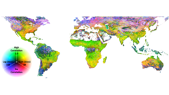
1. Introduction
Understanding the interconnection of biological and climatic processes is essential for predicting the effects of climate change on the biosphere. Vegetation phenology is a key indicator of climate-biosphere interactions. While it is feasible to model the interactions, models offer discrepant predictions of vegetation response to climate [1]. This indicates the need for better understanding of coupled vegetation-climate processes at a global scale. Although coarse-scale modeling may provide a synoptic picture of global phenology controls [1–3], observational data at high spatial and temporal resolution illustrate substantial local variations. Timings of phenology events have been associated with temperature [4,5] and precipitation [6] at continental aggregation scales to implicate climate trends in phenology shifts. However, the practice of associating shifts in arbitrarily defined events with climate indices can obfuscate complex interactions taking place over the entire growing season [7].
Plant growth has a strong, positive, though community-specific, correlation to precipitation events in arid regions [8,9], temperate regions [10–12] and water-limited ecosystems of Africa [13,14] and Australia [15]. In tropical ecosystems, some studies have shown low or negative correlation to precipitation [16,17], possibly as a result of light limitation, though other studies have questioned this supposition [18], and recent drought conditions in the Amazon have been associated with decreased greenness [19]. In contrast, temperature has a positive, strong association with vegetation in Northern, mid- to high latitudes [20–23]. In temperate grasslands that are not water limited, long-term vegetation production was linked to average growing season temperature [10]. Vegetation is also associated with air temperature at short time lags within the growing season [11,12]. This association is strong at the onset of the growth season, resulting in a correlation “wave” that moves north with time [22].
Previous studies have examined long-term relationships and anomalies between vegetation indices (VIs) and climate at a global scale [22], though with temporal (monthly) and spatial (one degree) aggregation that does not capture the local-scale diversity of phenological processes. These large spatio-temporal aggregations may not adequately or even correctly represent localized atmosphere-biosphere interactions [24]. The response to both temperature and precipitation varies spatio-temporally, according to the unique mixture of climatic and ecological processes operating at multiple scales [3,24,25]. The degree of spatial variability of the temporal response is not known. In areas of high biodiversity, such as the tropics, there may be substantial local variability due to changes in species composition [26]. Previous studies have not computed phenology response with sufficient spatio-temporal resolution to determine the usefulness of temporal information for global-scale mapping efforts.
The purpose of this study was a global characterization of observed (rather than modeled) vegetation response to observed climatic factors at fine temporal and spatial resolution. To achieve this, we avoided the use of thresholds on vegetation index, climatic factors or time and avoided the construction of timing events in the time series, which may or may not correspond well to phenological events on the ground [27,28]. We used lagged correlation (or cross-correlation) as a simple indicator of dominant land surface interactions with local climate [29,30]. We computed the lagged correlation of the Enhanced Vegetation Index (EVI) to cumulative Precipitation Estimation from Remotely Sensed Information using Artificial Neural Networks (PERSIANN) gridded rainfall [31] and land surface temperature (LST), between −60 to 60 degrees latitude at ∼4.4-kilometer and 1-kilometer resolution, respectively. We used only one threshold, EVI > 0, in the computation of correlations. The idea was to treat the data as a series, with the strength of relationship determined by both the magnitude and duration of temporally-matched events.
The maximum correlation, lag time to maximum and summation period for the maximum illustrate fine-grained evidence of ecosystem function. While much research has focused on land structure, in terms of land cover, biomass, etc., very little has focused on mapping land function. This project aims to partially fill that research gap.
2. Methods and Data
We used all available high quality data in calendar years 2008 to 2011 for the following data products. For EVI data, we used the Moderate Resolution Imaging Spectroradiometer (MODIS, on the Terra satellite) vegetation index product, MOD13A2 [32]. These data are 1-km spatial resolution in 16-day composites ( https://lpdaac.usgs.gov/products/modis_products_table/mod13a2). For every land pixel, we performed a quality control as described by [33], discarding pixels flagged as having low quality, shadows, clouds, adjacent clouds or high aerosols. For LST data, we used the MODIS (on the Aqua satellite) MYD11A2 thermal product. The LST data are 1-km spatial resolution in 8-day composites ( https://lpdaac.usgs.gov/products/modis_products_table/myd11a2). We used all pixels with an error <1 K according to the QA data, discarding pixels with larger uncertainty. For precipitation data, we used PERSIANN-Cloud Classification System (CCS) [31] daily rainfall, gridded at 0.04-degree (∼4.4 km at the Equator) resolution. PERSIANN no-data was indicated by a fill value. The extent of the PERSIANN data is nominally −60 to 60 degrees latitude, though we found a reduction in data density at high latitudes.
For each 1-kilometer EVI pixel, we extracted the covariate from under its centroid and computed cross correlation according to Equation (1):
In Equation (1), cov is the covariance function, computed according to methods described in [34], SD is the standard deviation, C is the covariate (either PERSIANN precipitation or MODIS LST), l is lag in days, t is the time in days (relative to 1 January 2008) of each EVI data point in a pixel, S is the summation period, s is a daily time step and ρl,S is the correlation between the EVI and the covariate at lag l, summed over S. The SD and covariance were evaluated over the set of all t for which data at both EVIt and ∑Ct−l−s existed. We computed the l and S at which the highest correlation occurs, where l was tested in weekly steps up to 168 days, for a maximum lag of 24 weeks, or 6 months, and S was tested in weekly time steps up to 84 days, for a maximum summation period of 12 weeks, or 3 months. Thus, correlations were evaluated between EVI and temperature or rainfall conditions as much as 168 + 84 days, or 9 months, prior to the observed EVI value. If the highest correlation was positive, it was returned along with the l and S at which the maximum occurred. If the highest correlation was negative, the lowest (most negative) correlation was returned along with l and S. We created maps of the correlation, l and S at which the maximum (or minimum) correlation occurred, as shown below.
We estimated the uncertainty of the correlation using the p-value of the correlation coefficient. Assuming that EVI and C are distributed according to a bivariate normal distribution and uncorrelated (true ρl,S = 0),
The code to implement this procedure in parallel is open source and available at [36].
We summarized correlation and lag globally by eco-region and biome according to the World Wildlife Fund (WWF) bioregional vector data [37] and the percentage of irrigated area [38]. The percentage of irrigated area is a global dataset representing the percent of area in 5 arc-minute pixels equipped for irrigation ( http://www.fao.org/nr/water/aquastat/irrigationmap/index10.stm). All available pixel data were used in these summaries, regardless of the p-value.
3. Results
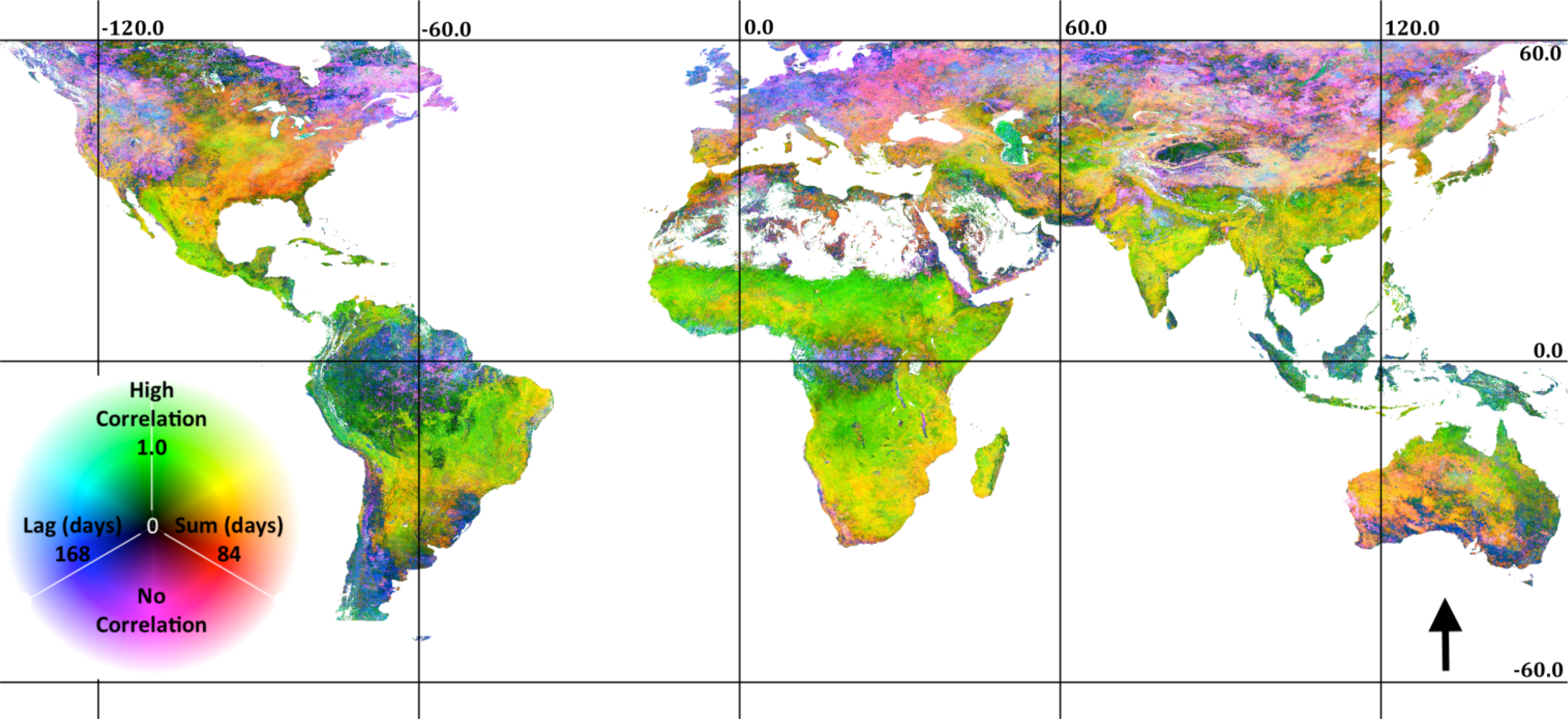
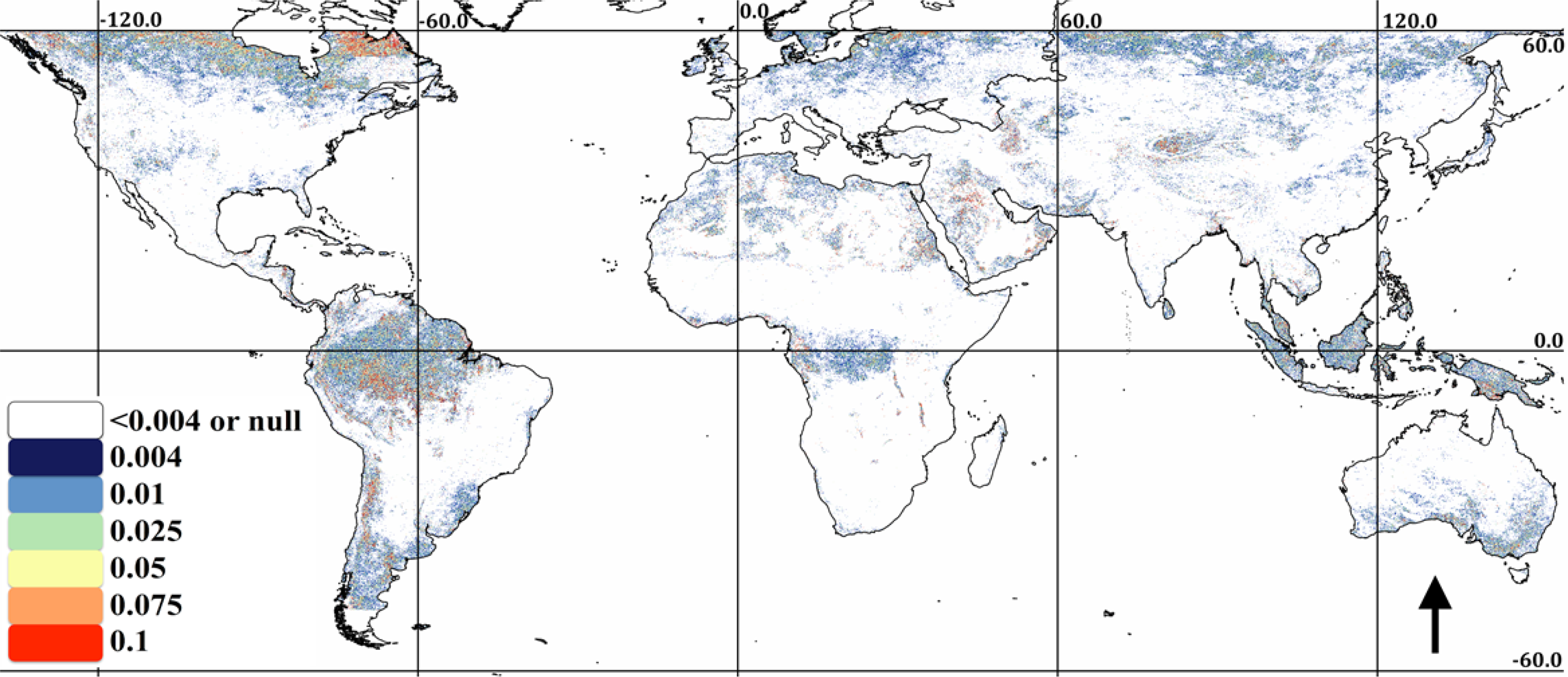
The association of EVI and PERSIANN precipitation is displayed in Figure 1. In Figure 1, ρl,S, l and S are displayed as an RGB composite, where green is set to correlation, blue is set to lag and red is set to summation period. As indicated in the legend, green areas indicate high correlation with a short lag and summation period; cyan areas indicate high correlation with a long lag; and yellow areas indicate high correlation and a long summation period and magenta or black areas indicating low to no correlation. This combination of temporal signals indicates herbaceous dominated ecosystems (the east-west band across sub-Saharan Africa and Eastern Brazil), water limited systems (Mexico) or rain-fed agriculture (India). Extreme northern and southern, as well as equatorial rainforest ecosystems have low correlation to precipitation at any lag or summation period. Negative correlations are extremely rare, though they are apparent in scattered maritime pixels on the west coast of South America and the Eastern Canadian Arctic. The p-values associated with the correlations are shown in Figure 2. Clearly, the majority of correlations are significant, though patches of low correlations may in fact be zero, as indicated by relatively high p-values. These patches are particularly evident in the Amazon, rain forest and boreal forest regions.
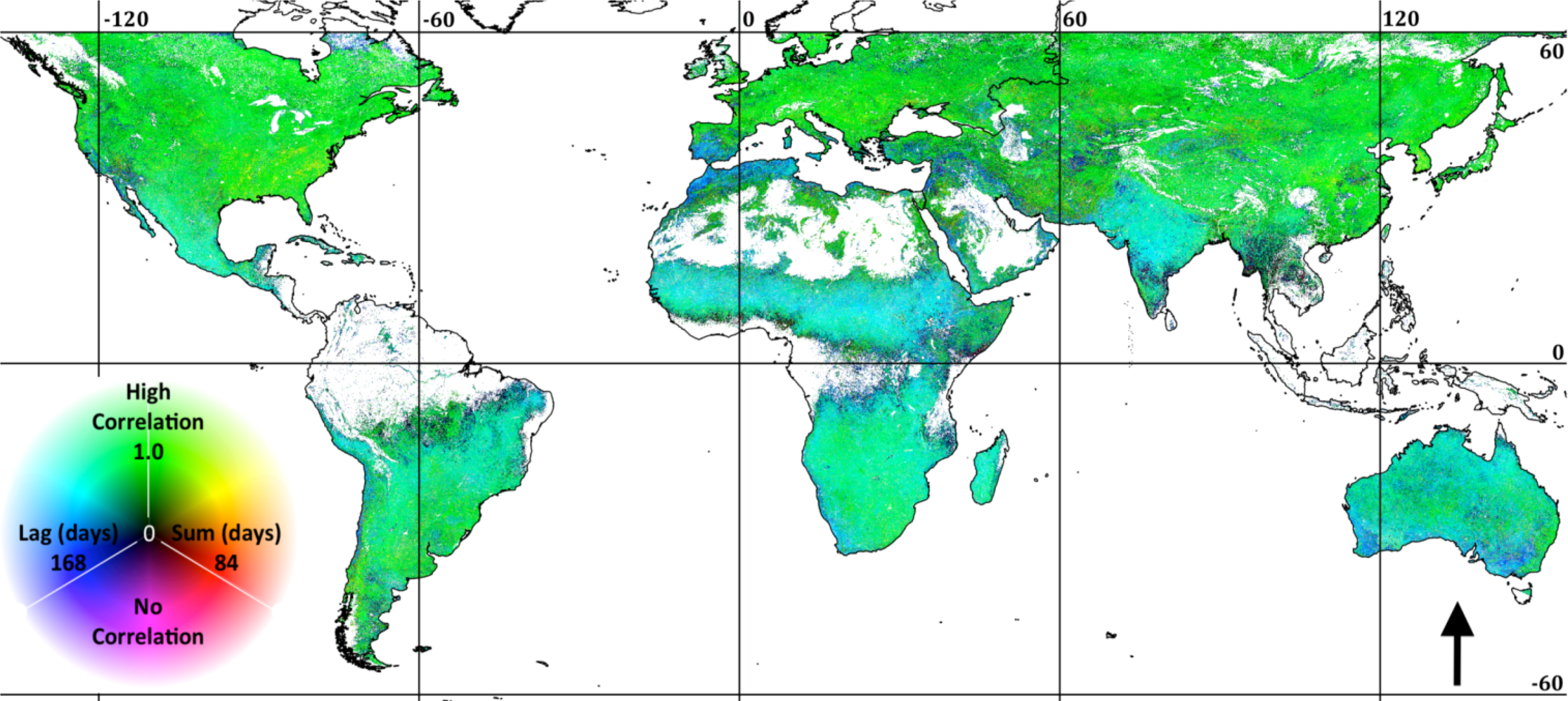
The association of EVI and MODIS LST is shown in Figure 3 (the same legend and color scheme as Figure 1). It is apparent from comparing Figures 1 and 3 that ecosystem association with temperature is much more predominant than precipitation, though interactions between climatic gradients and ecosystem type at the bioregional level result in a complex mosaic of phenological response to precipitation and temperature. In general, high latitude areas are highly correlated with temperature, while temperate and subtropical areas are more correlated with precipitation. However, extensive areas show a strong association to both temperature and rainfall, though at differing lags and summation periods. For example, Western Mexico is shown to have a rapid, strong response to precipitation, though also a strong response to temperature at a longer lag. The Southern USA is shown to have a strong association with temperature at a relatively short lag, though also a strong association to rainfall over a longer summation period. Unlike precipitation, extensive areas show a negative association to temperature (black in Figure 2), predominantly distributed in the tropics and Mediterranean climates. The p-values associated with the temperature correlations are shown in Figure 4. Due to the lower density of the data compared to the daily PERSIANN precipitation (reducing n in Equation (2)), there is a larger distribution of higher p-values (red), indicating possible zero correlation. Correlations close to zero also result in a high p-value. We found relatively high correlations in desert areas (e.g., North Africa and the Arabian Peninsula) derived from low variance, congruent seasonality in high LST and low EVI.
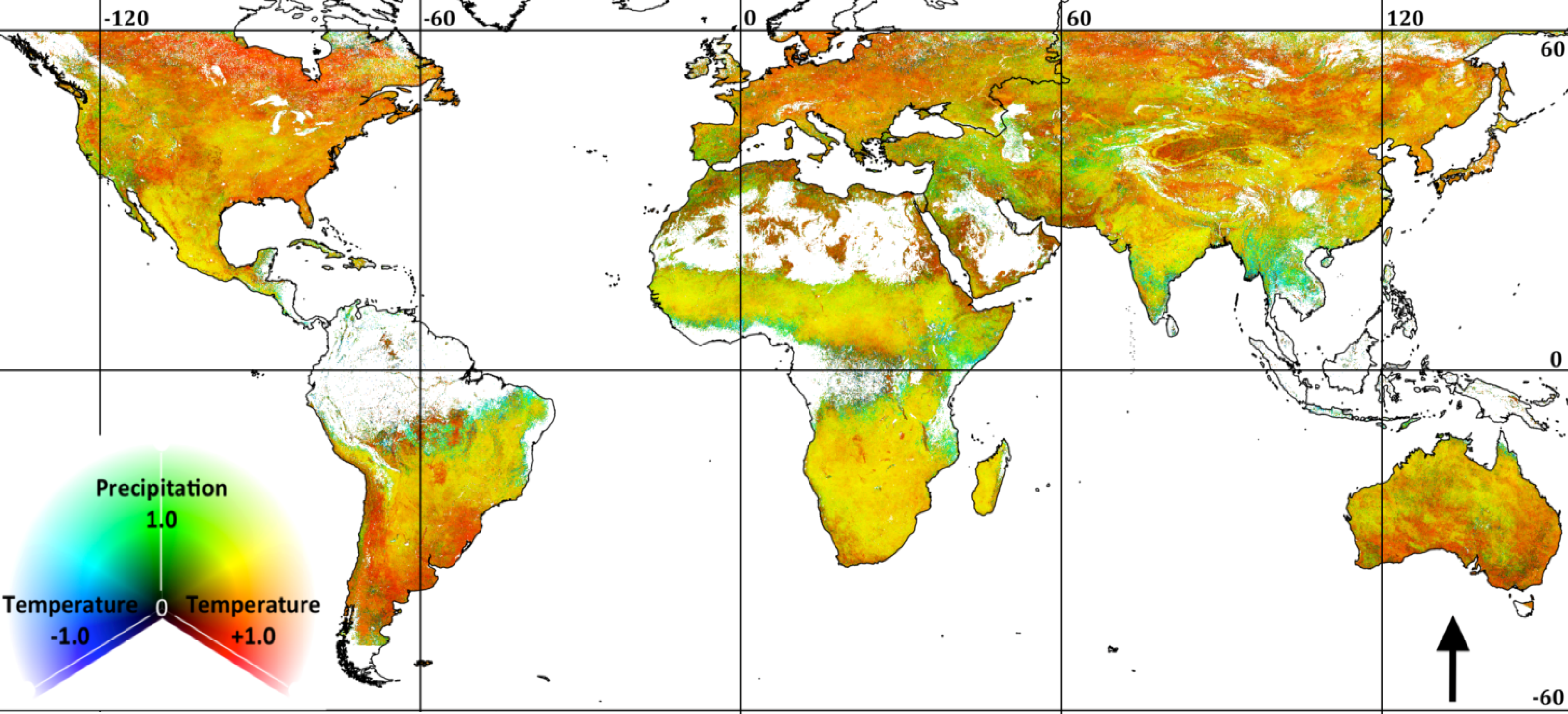
The balance between precipitation and temperature correlation is illustrated in Figure 5, where green areas indicate high correlation to precipitation, red areas indicate high positive correlation to temperature, blue areas indicate high negative correlation to temperature, yellow areas indicate high correlation to both rainfall and temperature and cyan areas indicate high correlation to rainfall and negative correlation to temperature. High correlations to precipitation are seen to dominate in southwest North America, the Mediterranean and portions of Australia. Large areas have a strong positive association with both temperature and precipitation (yellow), though the temporal timing of the correlations may differ. For example, Sub-Saharan Africa shows high correlation to precipitation at a short lag and summation period and also a high correlation to temperature at a long lag.
Summarizing the results by biome elucidates the influence of climatic zones. Mean values by biome are shown in Table 1 and SDs are shown in Table 2. Specifically, the highest correlations to precipitation (and shortest lags and summation periods) occur in tropical and subtropical biomes. This suggests that tropical biomes are affected by precipitation occurring approximately two months prior to the vegetation response, with the summation accounting for about six weeks and a lag of about two weeks. The lowest correlations to precipitation occur in boreal ecosystems, such as tundra and boreal forest. While these correlations are still relatively high (>0.5), the lags are very long (∼3 months) with long summation periods (∼50 days), indicating that antecedent moisture conditions may play a larger role than current season precipitation. By contrast, high latitude biomes have relatively high correlation to temperature, short lags (∼1 month) and very short summation periods of only a few days (“Tundra” and “Boreal Forests/Taiga” in Table 1). While the high latitude biomes have the shortest summation periods, other coniferous (both tropical and temperate) biomes also have high correlation to temperature and relatively short summation periods. The Mediterranean biome showed relatively low correlation to both precipitation and temperature. Table 2 shows some biomes to have a greater spread of phenology associations to temperature and precipitation. Specifically, tropical biomes show a relatively low SD for the precipitation correlation, while boreal biomes show a low SD for the temperature correlation.
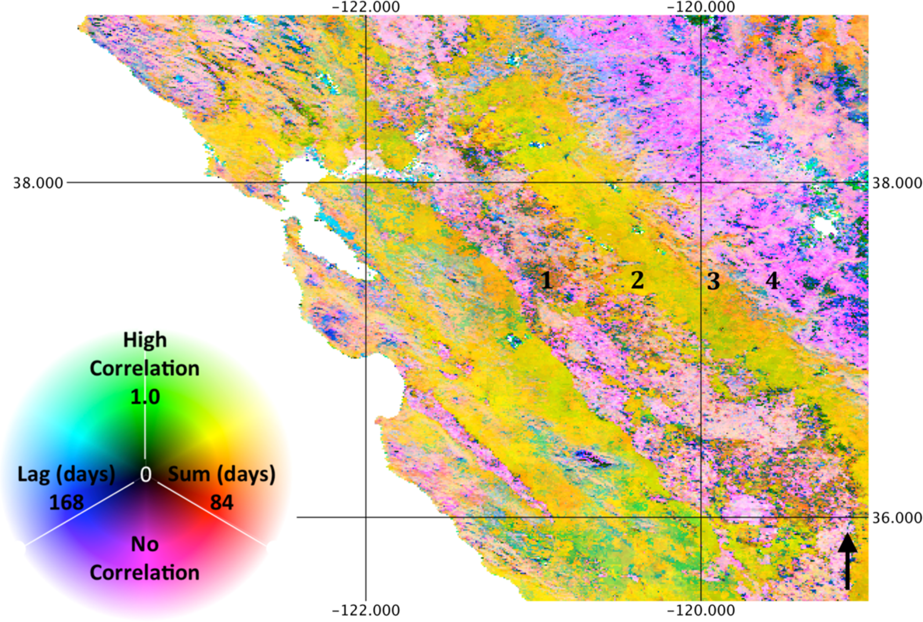
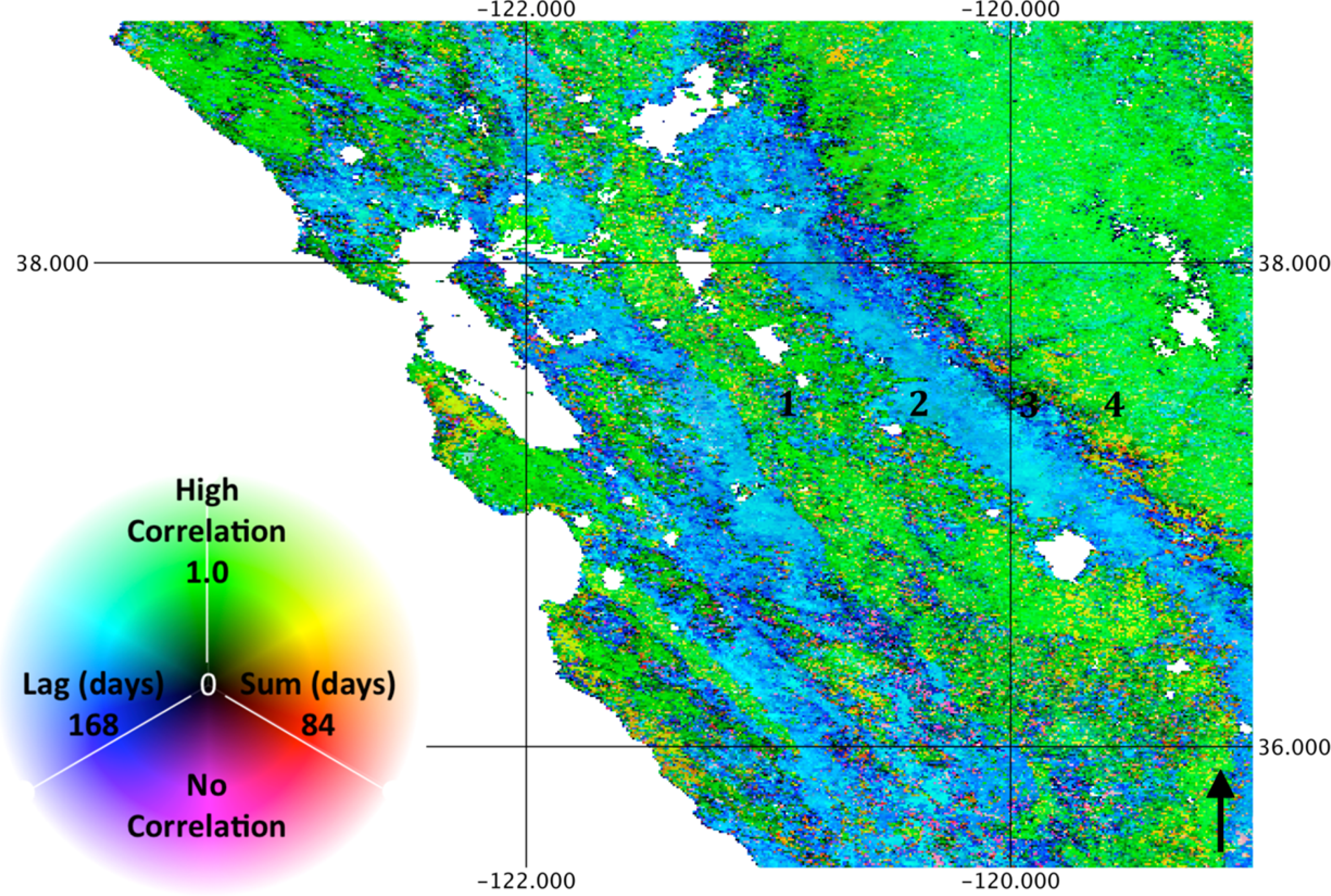
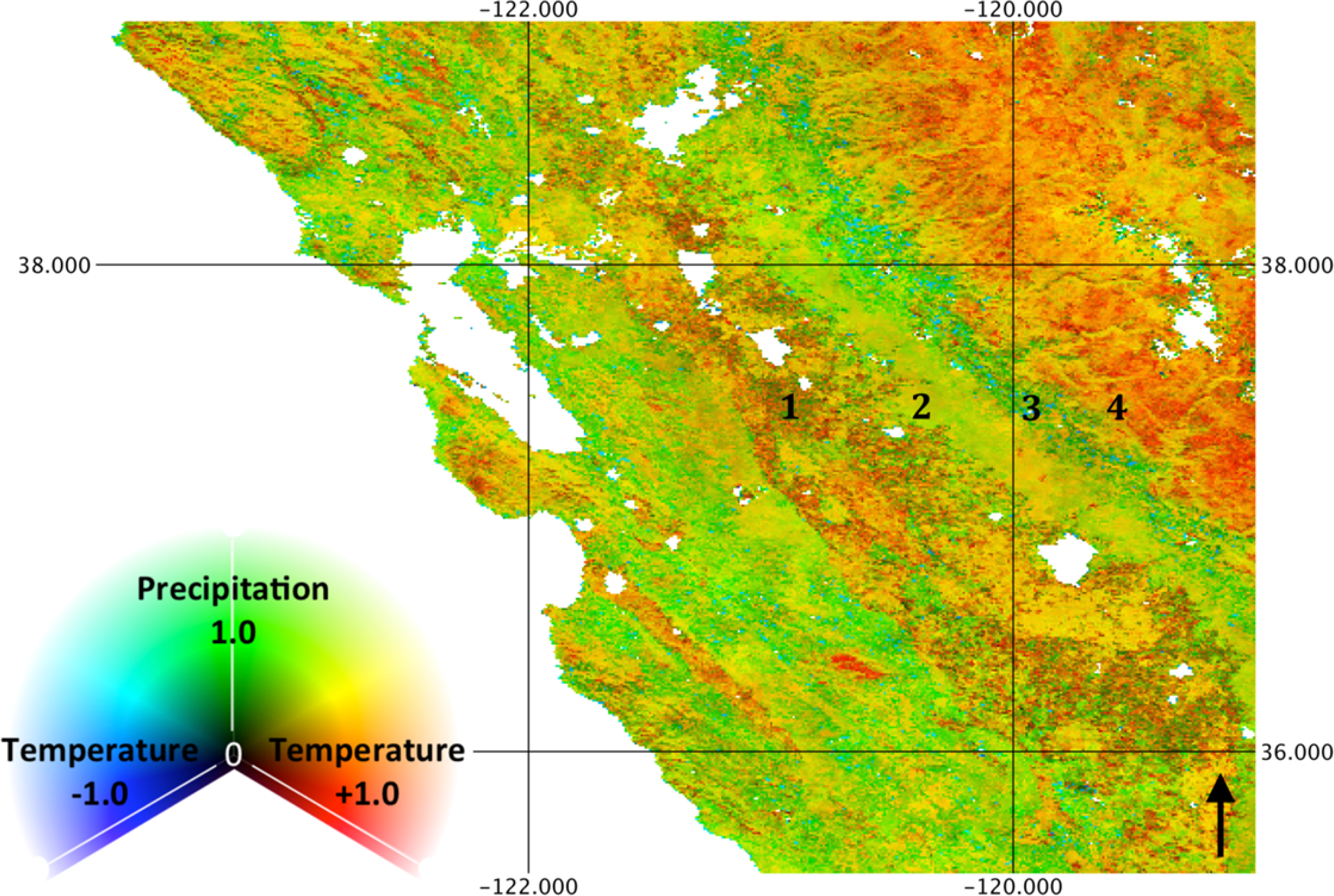
While biome level averages indicate a synoptic phenology at the global scale, the spatial patterns of correlation, lag and summation period at landscape scales indicate substantial local variability. These spatial patterns derive entirely from temporal information, suggesting that the remote sensing process can inform the prediction and understanding of ecosystem structure. For example, Figures 6 and 8 show the association with precipitation and LST, respectively, for the Mediterranean climate of the State of California, USA. The ecosystem function along an orographic gradient is distinct, as illustrated by the numbered locations. Specifically, at Location 1, irrigated agriculture in the central valley of California results in low correlation to precipitation and relatively high correlation to LST as cropping cycles correspond to the warm, dry season. Location 2, however, consists of primarily exotic annual grassland, characterized by rapid germination and growth in response to winter precipitation. As a result, high correlation to rainfall (with a short lag) and relatively low correlation to temperature with a long lag are observed. Location 3 consists of savanna and shrubland in the foothills of the Sierra Nevada Mountains, with intermediate correlation to precipitation, relatively long lags and summation periods and negative correlations to temperature in Sclerophyllous chaparral. At Location 4, the relatively high elevation mixed conifer forest experiences more abundant precipitation, thus a low correlation to rainfall and a high correlation to temperature. As this example illustrates, combinations of correlation and lag to precipitation and temperature are indicative of ecosystem form and function. While combinations of phenology response to precipitation and temperature coincide with land cover classes, transitions are far less abrupt, illustrating not only within-category variance of broad land cover types, but also ecotones that are difficult to represent though limited land cover categories.
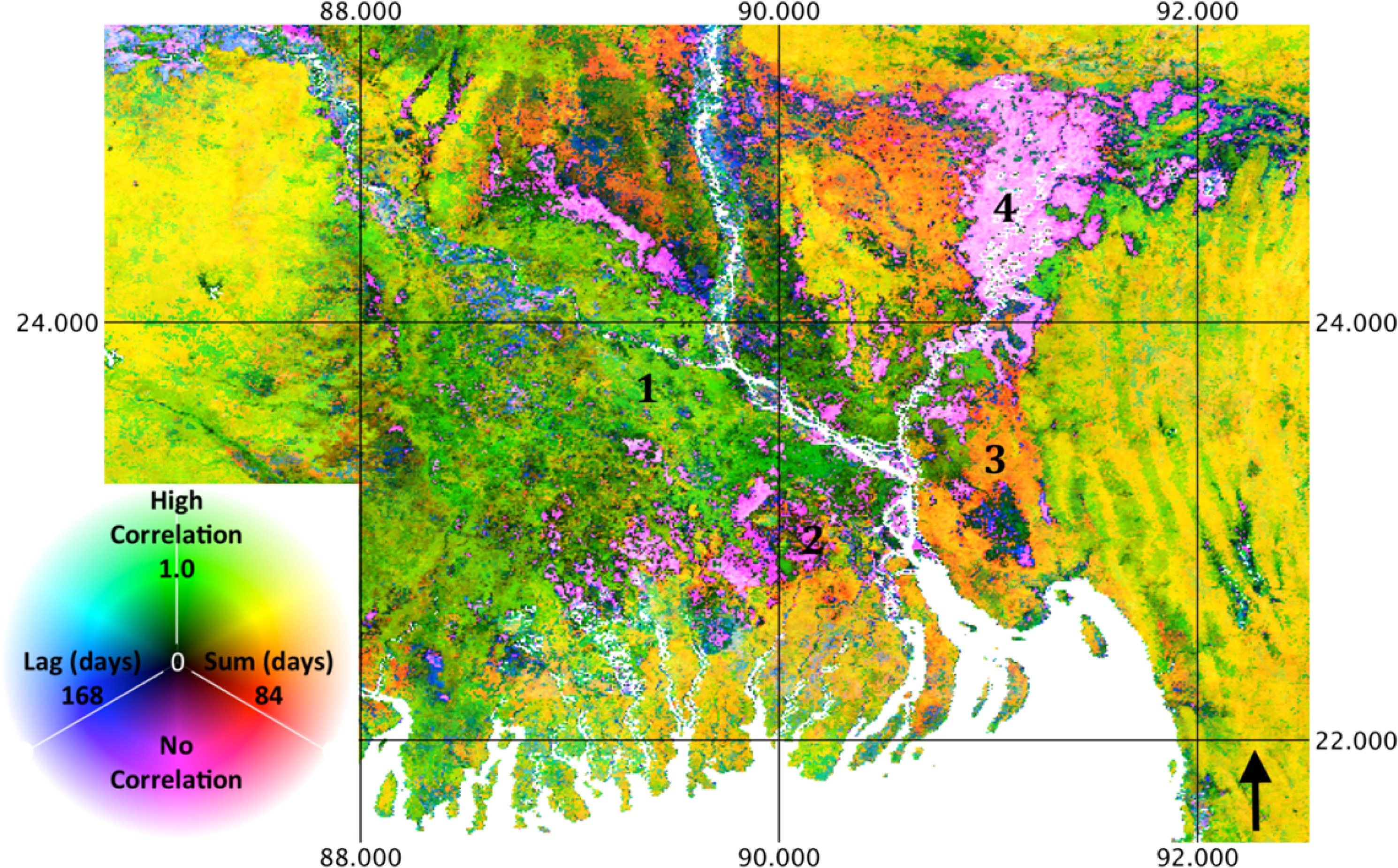
Figures 9 and 11 illustrate phenology differences in relation to precipitation and temperature in the Ganges River Delta area of Bangladesh. While the California example illustrates the correspondence of phenology response to land cover, Figures 9 and 11 illustrate substantially different phenology responses to climate variables within a category of land cover. At Location 1, a relatively high correlation to rainfall with a short lag and low or negative correlation to temperature indicates the cultivation of the transplanted Aman rice variety [39]. In contrast, Location 2 is characterized by low correlation to rainfall and high correlation to temperature, indicating cultivation of the transplanted Aus rice variety [39]. Location 3 experiences a high correlation to rainfall, though over an extended summation period, and a relatively high correlation to temperature, as well, indicating irrigated Rabi (hot, dry season) cropping. Location 4 is characterized by low correlation to rainfall and low to negative correlation to precipitation, indicating inundation and the susceptibility of crops to flooding [39]. While the MODIS land cover classifies the vast majority of this area as “cropland”, with no distinction, the results show substantial variation in vegetation phenology. This indicates that high-resolution phenology data may be useful for distinguishing irrigation intensity, crop type or agricultural rotations. It also suggests that ecosystem process information is supplementary to ecosystem structural information. In other words, land cover classification is an incomplete characterization of the surface, in that it omits temporal dynamics.
The relationship of precipitation and temperature correlations to area equipped for irrigation globally is shown in Figure 12. Not surprisingly, correlation to rainfall generally decreases with increasing access to irrigation infrastructure, as a result of uncoupling from local hydrologic conditions, though the highest percentages show an increase in correlation. This may be due to spatial autocorrelation: nearby irrigation infrastructure is replenished by rainfall or through the cultivation of water-intensive crops in highly irrigated areas, crops for which available water is partially supplied by irrigation, but augmented by precipitation. Correlation to temperature is seen to increase with area equipped for irrigation, suggesting that irrigated crops are more limited by temperature than by moisture availability.
4. Discussion
At macro-scale, our results are consistent with previous studies of global linkages between VIs and climatic factors [20,22]. Specifically, our results show that temperature is more influential at high latitudes [20] and that precipitation is limiting over broad regions of steppe, desert and grassland [10,12,21]. The correlation method is closely related to the Yearly Land Cover Dynamics (YLCD) method of [23] and shows similar results. However, the correlation method incorporates temporal information (lag and summation) and precipitation information not available from YLCD. Compared to process model estimated climatic controls on vegetation growth [1–3], it is apparent that the lagged association between observed vegetation and climate is roughly equivalent to model predicted limiting factors at broad spatial scales. However, our results represent observable evidence of global-scale ecosystem response to climate at a fine scale, as opposed to the output of models based on assumed processes.
Controlled experiments have shown a significant response of VIs to both precipitation and temperature in Mediterranean shrublands [40]. Despite the fact that correlation does not indicate causality, the results clearly indicate ecosystems in which rainfall triggers a relatively rapid growth response (high correlation, short lag, short summation period), for example in Western USA ecosystems infested by invasive annual grasses [29]. The combination of correlation, lag and summation period also correctly identifies ecosystems, such as temperate conifer forests (which we found to have the shortest mean lag and a relatively short, ∼1 week, summation period) previously shown to have a rapid response to surface temperature conditions [41]. Biomes such as Mediterranean ecosystems were less obviously characterized.
The fine spatial resolution results illustrate substantial local variation, both temporally and spatially. Previously, spatial aggregation at 0.5 degrees or larger scales [24,30], temporal aggregation at monthly [30] or seasonal [20] intervals or both spatial and temporal aggregation [42,43] have constrained phenology for informing land cover classifications or revealing local phenology variation. Our results suggest that higher resolution data can provide ecosystem process information at scales sufficient for local mapping of land use, cropping cycles, species composition or ecosystem function. For example, divergent community phenology signals have been shown to distinguish causes of deforestation [44] and invasive species infestation [29]. Compared to [45], relationships to precipitation and temperature in the Ganges River Delta reveal remarkably similar patterns. While [45] interpreted these patterns in terms of temporal endmembers (i.e., phenology as a mixture of periodic basis vectors), maximum cross-correlations contain different information (lag and summation period to both precipitation and temperature) and do not require a region of interest to be predefined (over which the spectral endmembers are valid).
That the correlations with temperature should be higher over broader portions of the global land surface than precipitation is at least in part due to our use of LST, rather than air temperature interpolated from observation stations. LST is not only an indicator of the environmental growing conditions, such as soil temperature, it is also a direct measurement of leaf temperature, which is an indicator of the physiological activity in vegetation [46]. However, as indicated in Table 1, the highest mean correlations to precipitation (tropical and subtropical dry broadleaf forests, grasslands, savannas and shrublands) are higher than the highest mean temperature correlations. This suggests that precipitation is more limiting than temperature, particularly in dry tropical and subtropical regions. While tropical ecosystems are also affected by temperature, both positively and negatively, a strong association at a short lag and summation period indicate that rapid germination and/or uptake strategies are essential for competitive advantage in moisture-limited ecosystems. This observation suggests that the potential effects of climate change need to be evaluated in terms of community-level composition, changing temperature and changing patterns of rainfall. Specifically, the increase of episodic events in areas of high correlation, a short lag and a short summation period (which we find to be primarily tropical and sub-tropical dry ecosystems) are likely to increase productivity and shift selective advantage.
Noise and error in the input data result in uncertainty in the reliability of the output for estimating phenology processes. Missing data in any of the inputs reduces the number of points used to compute cross-correlation, affecting the confidence with which the maximum correlation is estimated and, consequently, the summation period and lag to the presumed maximum correlation. Despite the use of quality flags to exclude noisy data, radiometric, estimation and retrieval errors remain in the remotely sensed data, possibly degrading the temporal input signals. For example, [18,47] show that EVI exhibits temporal patterns in the Amazon are related more to sun-target-sensor geometry than phenology. The cross-correlation is therefore affected by multiple error sources. Given this error and uncertainty, these data should be considered on a relative rather than absolute basis, for example in classification algorithms or as a continuous bioregional characterization, and interpreted with caution over tropical forest ecosystems with possibly strong anisotropic reflectance.
We anticipate several potential uses of these data in addition to land cover classifier inputs. One possibly beneficial application is in the validation of coupled biosphere-climate models. We suggest that biosphere-climate models should be able to simulate observed patterns as a first order check on appropriate coupling. If the coupled models are unable to reproduce the observed interaction, this is an indication of fundamental errors in the characterization of primary forcings on vegetative growth. While coupled models may not produce estimates of EVI, the near linear relationship between EVI and simulated landscape characteristics, such as LAI [32], should produce very similar lags and correlations. Another possible use is in the identification of places where climate change is likely to exert evolutionary pressure through shifts in competitive advantage. Climate variability represents a potentially strong extrinsic force on community composition and evolutionary force on local populations [48]. Climate factors have been shown to induce rapid, possibly irreversible transitions in community composition [49]. The phenology data may therefore indicate the geographic distribution of susceptibility to different types of climate variation (e.g., precipitation and temperature). Strong gradients in correlation, lag and/or summation period represent places where climate change is likely to have differential effects on different sides of the gradient. These places represent ecotones or community transitions that are likely to change spatial location in response to climatic forcing.
5. Conclusions
Here we used a simple correlation model with a minimum of assumptions as a data-driven approach to elucidating multi-scale dependencies on climatic factors. Specifically, correlations between four years of EVI data with time series of precipitation and land surface temperature reveal the spatio-temporal details of phenology at approximately four kilometers resolution and near global scope. Large area aggregations indicate high correlation, short lag and summation period response to precipitation in dry biomes, and high correlation short lag and summation period response to temperature in cold biomes. However, mapped results of maximum correlation, summation period and lag to maximum reveal phenological process variability never before observed at such high spatio-temporal resolution and broad spatial area. While the data are consistent with previous studies at regional and global scale, validation of the results are difficult, and high uncertainty will likely constrain the utility of the data in some locations and for some purposes. Promising pathways for future research involve a. monitoring such data over multiple time periods to determine whether observable changes in phenology correspond to climate or other external drivers, b. testing the ability of the phenology data to inform land cover or land use classifiers, c. estimation of climate change vulnerability from overlays of phenology gradients and predicted climate anomalies, d. validation of coupled atmosphere-biosphere models.
Acknowledgments
This research was partially supported by a National High Technology Grant from China (2009AA12200101).
Author Contributions
Nicholas Clinton conceived of the study, wrote code, performed the analysis and wrote the article, Le Yu performed the analysis. Haohuan Fu and Conghui He wrote code and processed the data, Peng Gong wrote the article.
Conflicts of Interest
The authors declare no conflict of interest.
References
- Churkina, G.; Running, S. Contrasting climatic controls on the estimated productivity of global terrestrial biomes. Ecosystems 1998, 1, 206–215. [Google Scholar]
- Nemani, R.R.; Keeling, C.D.; Hashimoto, H.; Jolly, W.M.; Piper, S.C.; Tucker, C.J.; Myneni, R.B.; Running, S.W. Climate-driven increases in global terrestrial net primary production from 1982 to 1999. Science 2003, 300, 1560–1563. [Google Scholar]
- Jolly, W.M.; Nemani, R.; Running, S.W. A generalized, bioclimatic index to predict foliar phenology in response to climate. Glob. Chang. Biol 2005, 11, 619–632. [Google Scholar]
- Myneni, R.; Keeling, C.; Tucker, C.; Asrar, G.; Nemani, R.R. Increased plant growth in the northern high latitudes from 1981 to 1991. Nature 1997, 386, 698–702. [Google Scholar]
- Zhou, L.; Tucker, C.J.; Kaufman, R.K.; Slayback, D.; Shabanov, N.; Myneni, R. Variations in northern vegetation activity inferred from satellite data of vegetation index during 1981 to 1999. J. Geophys. Res.: Atmos 2001. [Google Scholar] [CrossRef]
- Maignan, F.; Bréon, F.-M.; Bacour, C.; Demarty, J.; Poirson, A. Interannual vegetation phenology estimates from global AVHRR measurements. Remote Sens. Environ 2008, 112, 496–505. [Google Scholar]
- Angert, A; Biraud, S.; Bonfils, C.; Henning, C.C.; Buermann, W.; Pinzon, J.; Tucker, C.J.; Fung, I. Drier summers cancel out the CO2 uptake enhancement induced by warmer springs. Proc. Natl. Acad. Sci. USA 2005, 102, 10823–10827. [Google Scholar]
- Schmidt, H.; Karnieli, A. Remote sensing of the seasonal variability of vegetation in a semi-arid environment. J. Arid Environ 2000, 45, 43–59. [Google Scholar]
- Weiss, J.L.; Gutzler, D.S.; Coonrod, J.E.A.; Dahm, C.N. Long-term vegetation monitoring with NDVI in a diverse semi-arid setting, central New Mexico, USA. J. Arid Environ 2004, 58, 249–272. [Google Scholar]
- Piao, S.; Friedlingstein, P.; Ciais, P.; Viovy, N.; Demarty, J. Growing season extension and its impact on terrestrial carbon cycle in the Northern Hemisphere over the past 2 decades. Glob. Biogeochem. Cycles 2007. [Google Scholar] [CrossRef]
- Wang, J.; Price, K.P.; Rich, P.M. Spatial patterns of NDVI in response to precipitation and temperature in the central Great Plains. Int. J. Remote Sens 2001, 22, 3827–3844. [Google Scholar]
- Wang, J.; Rich, P.M.; Price, K.P. Temporal responses of NDVI to precipitation and temperature in the central Great Plains, USA. Int. J. Remote Sens 2003, 24, 2345–2364. [Google Scholar]
- Zhang, X. Monitoring the response of vegetation phenology to precipitation in Africa by coupling MODIS and TRMM instruments. J. Geophys. Res.: Atmos 2005. [Google Scholar] [CrossRef]
- Gaughan, A.; Stevens, F. Linking vegetation response to seasonal precipitation in the Okavango–Kwando–Zambezi catchment of southern Africa. Int. J. Remote Sens 2012, 33, 37–41. [Google Scholar]
- Wong, W.F.J. Spatial and temporal analysis of MODIS EVI and TRMM 3B43 rainfall retrievals in Australia. Proceeding of the 2011 19th International Conference on Geoinformatics, Shanghai, China, 24–26 June 2011; pp. 1–7.
- Restrepo-Coupe, N.; da Rocha, H.R.; Hutyra, L.R.; da Araujo, A.C.; Borma, L.S.; Christoffersen, B.; Cabral, O.M.R.; de Camargo, P.B.; Cardoso, F.L.; da Costa, A.C.L.; et al. What drives the seasonality of photosynthesis across the Amazon basin? A cross-site analysis of eddy flux tower measurements from the Brasil flux network. Agric. For. Meteorol 2013, 182–183, 128–144. [Google Scholar]
- Lee, J.; Frankenberg, C.; Berry, J.A.; Boyce, C.K.; Fisher, J.B.; Morrow, E.; Worden, J.R.; Asefi, S.; Badgley, G.; Saatchi, S.; et al. Forest productivity and water stress in Amazonia: Observations from GOSAT chlorophyll fluorescence. Proc. R. Soc. B Biol. Sci 2013, 280, 10823–10827. [Google Scholar]
- Morton, D.C.; Nagol, J.; Carabajal, C.C.; Rosette, J.; Palace, M.; Cook, B.D.; Vermote, E.F.; Harding, D.J.; North, P.R.J. Amazon forests maintain consistent canopy structure and greenness during the dry season. Nature 2014, 506, 221–224. [Google Scholar]
- Xu, L.; Samanta, A.; Costa, M.H.; Ganguly, S.; Nemani, R.R.; Myneni, R.B. Widespread decline in greenness of Amazonian vegetation due to the 2010 drought. Geophys. Res. Lett 2011. [Google Scholar] [CrossRef]
- Ichii, K.; Kawabata, A.; Yamaguchi, Y. Global correlation analysis for NDVI and climatic variables and NDVI trends: 1982–1990. Int. J. Remote Sens 2002, 23, 3873–3878. [Google Scholar]
- Zhang, X.; Friedl, M.A.; Schaaf, C.B.; Strahler, A.H. Climate controls on vegetation phenological patterns in northern mid- and high latitudes inferred from MODIS data. Glob. Chang. Biol 2004, 10, 1133–1145. [Google Scholar]
- Zeng, F.-W.; Collatz, G.; Pinzon, J.; Ivanoff, A. Evaluating and quantifying the climate-driven interannual variability in Global Inventory Modeling and Mapping Studies (GIMMS) Normalized Difference Vegetation Index (NDVI3g) at global scales. Remote Sens 2013, 5, 3918–3950. [Google Scholar]
- Julien, Y.; Sobrino, J.A. The Yearly Land Cover Dynamics (YLCD) method: An analysis of global vegetation from NDVI and LST parameters. Remote Sens. Environ 2009, 113, 329–334. [Google Scholar]
- Horion, S.; Cornet, Y.; Erpicum, M.; Tychon, B. Studying interactions between climate variability and vegetation dynamic using a phenology based approach. Int. J. Appl. Earth Obs. Geoinf 2013, 20, 20–32. [Google Scholar]
- Peñuelas, J.; Filella, I.; Zhang, X. Complex spatiotemporal shifts as a response to rainfall changes. New Phytol 2004, 161, 837–846. [Google Scholar]
- Borchert, R. Responses of tropical trees to rainfall seasonality and its long-term changes. Clim. Chang 1998, 39, 381–393. [Google Scholar]
- Cleland, E.E.; Chuine, I.; Menzel, A.; Mooney, H.A.; Schwartz, M.D. Shifting plant phenology in response to global change. Trends Ecol. Evol 2007, 22, 357–365. [Google Scholar]
- Morisette, J.T.; Richardson, A.D.; Knapp, A.K.; Fisher, J.I.; Graham, E.A; Abatzoglou, J.; Wilson, B.E.; Breshears, D.D.; Henebry, G.M.; Hanes, J.M.; et al. Tracking the rhythm of the seasons in the face of global change: Phenological research in the 21st century. Front. Ecol. Environ 2009, 7, 253–260. [Google Scholar]
- Clinton, N.E.; Potter, C.; Crabtree, B.; Genovese, V.; Gross, P.; Gong, P. Remote sensing-based time-series analysis of cheatgrass (Bromus tectorum L.) phenology. J. Environ. Qual 2010, 39, 955–963. [Google Scholar]
- Brunsell, N. Characterization of land-surface precipitation feedback regimes with remote sensing. Remote Sens. Environ 2006, 100, 200–211. [Google Scholar]
- Hong, Y.; Hsu, K.-L.; Sorooshian, S.; Gao, X. Precipitation estimation from remotely sensed imagery using an artificial neural network cloud classification system. J. Appl. Meteorol 2004, 43, 1834–1852. [Google Scholar]
- Huete, A.; Didan, K.; Miura, T.; Rodriguez, E.P.; Gao, X.; Ferreira, L.G. Overview of the radiometric and biophysical performance of the MODIS vegetation indices. Remote Sens. Environ 2002, 83, 195–213. [Google Scholar]
- Samanta, A.; Ganguly, S.; Vermote, E.; Nemani, R.R.; Myneni, R.B. Interpretation of variations in MODIS-measured greenness levels of Amazon forests during 2000 to 2009. Environ. Res. Lett 2012. [Google Scholar] [CrossRef]
- Pébay, P. Formulas for Robust, One-Pass Parallel Computation of Covariances and Arbitrary-Order Statistical Moments; Sandia Rep. SAND2008-6212; Sandia Natl. Lab.: Albuquerque, NM, USA/Livermore, CA, USA, 2008. [Google Scholar]
- Hotelling, H. New light on the correlation coefficient and its transforms. J. R. Stat. Soc. Ser. B 1953, 15, 193–232. [Google Scholar]
- Java-Remote-Sensing-Tools. Available online: https://code.google.com/p/java-remote-sensingtools/source/browse/trunk/Open/src/cn/edu/tsinghua/timeseries/Correlatr3.java (accessed on 28 July 2014).
- Olson, D.M.; Dinerstein, E.; Wikramanayake, E.D.; Burgess, N.D.; Powell, G.V.N.; D’Amico, J.A.; Itoua, I.; Strand, H.E.; Morrison, J.C.; Loucks, C.J.; et al. Terrestrial ecoregions of the world: A new map of life on earth. Bioscience 2001, 51, 933–938. [Google Scholar]
- Siebert, S.; Döll, P.; Hoogeveen, J.; Faures, J.-M.; Frenken, K.; Feick, S. Development and validation of the global map of irrigation areas. Hydrol. Earth Syst. Sci 2005, 2, 1299–1327. [Google Scholar]
- Sattar, S.A. Bridging the rice yield gap in Bangladesh. In Bridging the Rice Yield Gap in the Asia-Pacific Region; Papademetriou, M.K., Dent, F.J., Herath, E.M., Eds.; FAO: Bangkok, Thailand, 2000. [Google Scholar]
- Filella, I. Reflectance assessment of seasonal and annual changes in biomass and CO2 uptake of a Mediterranean shrubland submitted to experimental warming and drought. Remote Sens. Environ 2004, 90, 308–318. [Google Scholar]
- Wu, J.; Guan, D.; Yuan, F.; Wang, A.; Jin, C. Soil temperature triggers the onset of photosynthesis in Korean pine. PLoS One 2013. [Google Scholar] [CrossRef]
- White, M.A.; Nemani, R.R. Real-time monitoring and short-term forecasting of land surface phenology. Remote Sens. Environ 2006, 104, 43–49. [Google Scholar]
- Hüttich, C.; Gessner, U.; Herold, M.; Strohbach, B.J.; Schmidt, M.; Keil, M.; Dech, S. On the suitability of MODIS time series metrics to map vegetation types in dry savanna ecosystems: A case study in the Kalahari of NE Namibia. Remote Sens 2009, 1, 620–643. [Google Scholar]
- Morton, D.C.; DeFries, R.S.; Shimabukuro, Y.E.; Anderson, L.O.; Arai, E.; Freitas, R.; del Bon Espirito-Santo, F.; Morisette, J. Cropland expansion changes deforestation dynamics in the southern Brazilian Amazon. Proc. Natl. Acad. Sci. USA 2006, 103, 14637–14641. [Google Scholar]
- Small, C. Spatiotemporal dimensionality and Time-Space characterization of multitemporal imagery. Remote Sens. Environ 2012, 124, 793–809. [Google Scholar]
- Sims, D.; Rahman, A.; Cordova, V.; Elmasri, B.; Baldocchi, D.; Bolstad, P.; Flanagan, L.; Goldstein, A; Hollinger, D.; Misson, L.; et al. A new model of gross primary productivity for North American ecosystems based solely on the enhanced vegetation index and land surface temperature from MODIS. Remote Sens. Environ 2008, 112, 1633–1646. [Google Scholar]
- Galvão, L.S.; dos Santos, J.R.; Roberts, D.A.; Breunig, F.M.; Toomey, M.; de Moura, Y.M. On intra-annual EVI variability in the dry season of tropical forest: A case study with MODIS and hyperspectral data. Remote Sens. Environ 2011, 115, 2350–2359. [Google Scholar]
- Reyer, C.P.O.; Leuzinger, S.; Rammig, A.; Wolf, A.; Bartholomeus, R.P.; Bonfante, A.; de Lorenzi, F.; Dury, M.; Gloning, P.; Abou Jaoudé, R.; et al. A plant’s perspective of extremes: Terrestrial plant responses to changing climatic variability. Glob. Chang. Biol 2013, 19, 75–89. [Google Scholar]
- Breshears, D.D.; Cobb, N.S.; Rich, P.M.; Price, K.P.; Allen, C.D.; Balice, R.G.; Romme, W.H.; Kastens, J.H.; Floyd, M.L.; Belnap, J.; et al. Regional vegetation die-off in response to global-change-type drought. Proc. Natl. Acad. Sci. USA 2005, 102, 15144–15148. [Google Scholar]


| Precipitation | Temperature | |||||
|---|---|---|---|---|---|---|
| Corr. | Lag | Sum | Corr. | Lag | Sum | |
| Tropical and Subtropical Moist Broadleaf Forests | 0.59 | 51 | 35 | 0.24 | 56 | 9 |
| Tropical and Subtropical Dry Broadleaf Forests | 0.76 | 21 | 49 | 0.22 | 78 | 11 |
| Tropical and Subtropical Coniferous Forests | 0.73 | 15 | 50 | 0.69 | 88 | 13 |
| Temperate Broadleaf and Mixed Forests | 0.56 | 90 | 60 | 0.58 | 35 | 8 |
| Temperate Conifer Forests | 0.56 | 98 | 56 | 0.62 | 30 | 10 |
| Boreal Forests/Taiga | 0.51 | 112 | 52 | 0.63 | 39 | 2 |
| Tropical and Subtropical Grasslands, Savannas and Shrublands | 0.75 | 15 | 45 | 0.48 | 93 | 10 |
| Temperate Grasslands, Savannas and Shrublands | 0.57 | 81 | 55 | 0.50 | 48 | 6 |
| Flooded Grasslands and Savannas | 0.62 | 47 | 48 | 0.51 | 70 | 10 |
| Montane Grasslands and Shrublands | 0.68 | 71 | 57 | 0.61 | 60 | 9 |
| Tundra | 0.61 | 123 | 52 | 0.59 | 38 | 2 |
| Mediterranean Forests, Woodlands and Scrub | 0.54 | 64 | 54 | 0.26 | 90 | 10 |
| Deserts and Xeric Shrublands | 0.59 | 60 | 56 | 0.44 | 64 | 11 |
| Mangroves | 0.61 | 57 | 33 | 0.01 | 54 | 10 |
| Precipitation | Temperature | |||||
|---|---|---|---|---|---|---|
| Corr. | Lag | Sum | Corr. | Lag | Sum | |
| Tropical and Subtropical Moist Broadleaf Forests | 0.19 | 57 | 31 | 0.60 | 47 | 20 |
| Tropical and Subtropical Dry Broadleaf Forests | 0.15 | 35 | 25 | 0.69 | 51 | 22 |
| Tropical and Subtropical Coniferous Forests | 0.15 | 24 | 25 | 0.37 | 43 | 25 |
| Temperate Broadleaf and Mixed Forests | 0.14 | 55 | 27 | 0.41 | 41 | 22 |
| Temperate Conifer Forests | 0.16 | 57 | 29 | 0.37 | 36 | 23 |
| Boreal Forests/Taiga | 0.17 | 55 | 31 | 0.40 | 44 | 12 |
| Tropical and Subtropical Grasslands, Savannas and Shrublands | 0.14 | 27 | 24 | 0.49 | 48 | 22 |
| Temperate Grasslands, Savannas and Shrublands | 0.16 | 56 | 29 | 0.43 | 43 | 19 |
| Flooded Grasslands and Savannas | 0.19 | 55 | 29 | 0.47 | 49 | 23 |
| Montane Grasslands and Shrublands | 0.18 | 55 | 28 | 0.38 | 47 | 22 |
| Tundra | 0.18 | 41 | 29 | 0.47 | 50 | 11 |
| Mediterranean Forests, Woodlands and Scrub | 0.16 | 55 | 31 | 0.53 | 61 | 23 |
| Deserts and Xeric Shrublands | 0.18 | 51 | 30 | 0.42 | 53 | 25 |
| Mangroves | 0.18 | 52 | 31 | 0.58 | 49 | 21 |
© 2014 by the authors; licensee MDPI, Basel, Switzerland This article is an open access article distributed under the terms and conditions of the Creative Commons Attribution license (http://creativecommons.org/licenses/by/3.0/).
Share and Cite
Clinton, N.; Yu, L.; Fu, H.; He, C.; Gong, P. Global-Scale Associations of Vegetation Phenology with Rainfall and Temperature at a High Spatio-Temporal Resolution. Remote Sens. 2014, 6, 7320-7338. https://doi.org/10.3390/rs6087320
Clinton N, Yu L, Fu H, He C, Gong P. Global-Scale Associations of Vegetation Phenology with Rainfall and Temperature at a High Spatio-Temporal Resolution. Remote Sensing. 2014; 6(8):7320-7338. https://doi.org/10.3390/rs6087320
Chicago/Turabian StyleClinton, Nicholas, Le Yu, Haohuan Fu, Conghui He, and Peng Gong. 2014. "Global-Scale Associations of Vegetation Phenology with Rainfall and Temperature at a High Spatio-Temporal Resolution" Remote Sensing 6, no. 8: 7320-7338. https://doi.org/10.3390/rs6087320
APA StyleClinton, N., Yu, L., Fu, H., He, C., & Gong, P. (2014). Global-Scale Associations of Vegetation Phenology with Rainfall and Temperature at a High Spatio-Temporal Resolution. Remote Sensing, 6(8), 7320-7338. https://doi.org/10.3390/rs6087320