1. Introduction
Defined as one-half of the total green leaf area (all-sided) per unit ground surface area [
1], the leaf area index (LAI) is an important parameter and is commonly applied in environmental studies examining growth monitoring, yield estimation, evapotranspiration, radiation extinction, carbon cycling and climate [
2–
5]. Direct measurement of the LAI via the use of destructive field measurements is extremely labor intensive, tedious and limited to experimental plots. Remote sensing techniques have been recognized as a reliable method to provide a fast, non-destructive and relatively cheap way to measure LAI on different scales [
6,
7].
Hyperspectral remote sensing can produce hundreds or even thousands of narrow, contiguous spectral bands, which may provide crucial additional information, potentially representing a significant improvement over broad bands in quantifying biophysical and biochemical variables, such as LAI [
8,
9]. However, hyperspectral data are much more complex than multispectral data. Although they provide a vast amount of information, most adjacent wavebands are redundant and often highly correlated [
10]. It is therefore essential to determine the best spectral features derived from hyperspectral data in order to accurately quantify LAI.
Various methods have been proposed, applied and improved in recent decades for the extraction of the spectral features of hyperspectral information. These selection techniques can be classified into three broad groups. (i) Waveband features: Compared with broad bands, narrow bands in specific portions of the spectrum are known to improve discrimination capabilities for various vegetation. Thenkabail
et al. [
10] determined 22 optimal hyperspectral wavebands with which to best characterize vegetation and agricultural crops over the spectral range of 400–2500 nm. Becker
et al. [
11] used second-derivative analysis to identify eight optimal spectral bands in the visible-NIR wavelength region that appeared to contain the majority of the coastal wetland information content of the full spectral resolution. Wang
et al. [
12] employed three methods, including correlation coefficient-based, vegetation index-based and the stepwise regression method to select 15 suitable wavebands for paddy rice LAI estimation. (ii) Spectral position features: Reflectance and absorption features that characterize hyperspectral data are also related to specific physical and chemical crop characteristics [
13]. Pu
et al. [
14] found strong correlations between forest LAI and various red-edge parameters, including the red-edge position (REP) and the red-well position (RWP). Spectral features in the shortwave infrared (SWIR) regions (as well as those in the near-infrared) are also important in predicting LAI [
9,
15]. (iii) Vegetation indices: Spectral vegetation indices are mathematical combinations of different spectral bands, mostly in the visible and near-infrared regions of the electromagnetic spectrum. Although the normalized difference vegetation index (NDVI) is by far the most well-known and widely used method of estimating LAI [
16], it is sensitive to soil and saturates at a relatively low LAI level. In contrast, VIs, such as the soil adjusted vegetation index (SAVI; [
17]), second modified SAVI (MSAVI2; [
18]), renormalized difference vegetation index (RDVI; [
19]) and triangular vegetation index (TVI; [
20]), have now been devised to improve LAI estimation. It also has been demonstrated that VIs with red-edge bands are good predictors of widely variable green LAI, such as CI
Red-edge [
21,
22].
The above-mentioned studies have made important progresses in detecting canopy information via the use of hyperspectral remote sensing. However, the research that systematically summarizes and analyzes the different spectral features of hyperspectral remote sensing data in terms of their performance in estimating LAI is rare, with the analysis of a single feature typically not sufficient to explore such rich information. Several studies have focused on statistical techniques, such as stepwise multiple linear regression (SMLR), which makes use of the information provided by several spectral features to estimate biochemical and biophysical vegetation properties [
23,
24]. In either case, multi-collinearity is a common problem inherent to hyperspectral datasets [
25].
Partial least squares regression (PLSR) is a data compression technique that reduces a large number of collinear variables to a few non-correlated latent variables or factors [
26–
28]. A number of studies have shown that PLSR is a powerful tool able to extract significant signals and to create reliable models [
8,
29–
32], and it has the potential to accurately predict LAI. Although these previous studies employed all available spectral wavelengths simultaneously for PLSR, others have revealed that the use of only a few features is sufficient to extract and discriminate essential information and characteristics [
10]. As the use of full spectral subsets or the greatest available amount of spectral information would likely not improve retrieval performance, but simply increase computation time [
24], it may therefore be more effective to obtain the most accurate biophysical vegetation data possible to build the model.
The objectives of this study were to: (1) systematically summarize the spectral features of hyperspectral canopy reflectance in terms of three aspects: feature wavebands, feature positions and vegetation indices; (2) evaluate every feature’s potential for LAI estimation; and (3) identify optimal features (and their numbers) for LAI estimation via PLSR.
4. Discussion
To obtain adequate information from hyperspectral data, many features were identified based on spectral wavebands, spectral positions and vegetation indices. Additionally, the correlations between these features and wheat LAI values were studied. The analysis of the spectral waveband features revealed important features correlating with LAI across a broad range. However, compared to the performance of data produced via first derivative analysis, as well as absorption and reflectance position features and vegetation indices, the spectral features exhibited lower correlation coefficients, due to the influence of external factors, such as underlying soil brightness, leaf angle distribution and leaf optical properties [
15,
24].
The red-edge region is characterized by a sharp rise in the reflectance of green vegetation between the local minimum reflectance band in the red spectral region and the maximum reflectance band in the NIR spectral region. This region is considered to contain more information regarding biomass quantity and LAI than other parts of the electromagnetic spectrum [
64,
65]. In this study, many spectral features identified in the red-edge region had high precision and were more accurate (
i.e., FD3, CI
Red-edge and A_Area
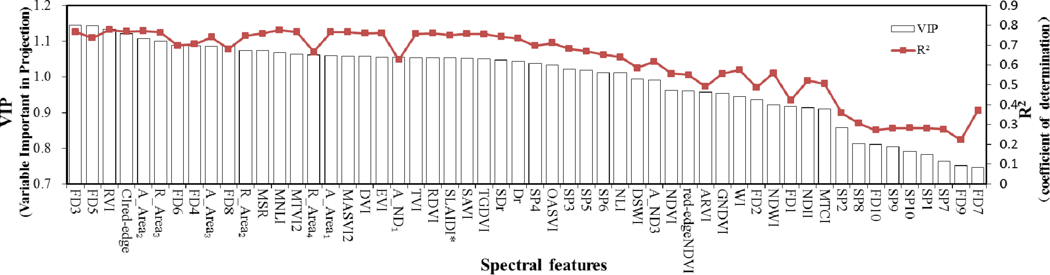
1). FD3 was the first derivative at a wavelength of 750 nm and had both the strongest correlation with LAI (
R2 = 0.800) and the highest VIP value (VIP = 1.144) of all features. This confirmed previous findings by Wang
et al. [
12] with 723 nm and Thenkabail
et al. [
10] with 735 nm. CI
Red-edge led to an
R2 of 0.766 and a VIP of 1.121, which was more sensitive to LAI variability than the NDVI. Viña [
21] also showed that the CI
Red-edge exhibited low sensitivity to soil background effects, and it constitutes a simple, yet robust tool for the remote and synoptic estimation of green LAI.
In the NIR region (800–1300 nm), reflectance spectra and first derivative spectra (SP4, SP5, FD4 and FD5), absorption and reflectance features (R_Area
3, A_Area
3, A_Area
2, R_Area
2 and R_Area
4) and most vegetation indices (RVI, EVI, DVI and MTVI2) performed more effectively. The reflectance in this spectral region is mainly influenced by the arrangement of cells within the mesophyll layer of leaves, as well as by canopy structure, especially the number of vertical leaf layers. NIR water absorption regions are also sensitive to leaf moisture content [
12].
The advantage of vegetation indices is that they can be used to obtain relevant information rapidly and easily, and the underlying mechanisms are well-understood [
66]. For the 24 VIs examined in this study, NDVI had a lower accuracy than most of the studied vegetation indices. The obtained results are in agreement with those found elsewhere in the literature [
5,
16,
42]. Most modified vegetation indices were better than their respective originals, including: MNLI
vs. NLI, MSAVI2
vs. SAVI and RDVI
vs. DVI, which is consistent with previous studies [
18,
19,
42]. Some vegetation indices based on three discrete bands also produced strong correlation, including the following: EVI, TVI, TGDVI, MTVI2 and sLAIDI
*, which take advantage of sensitive spectral regions to reduce external factor and are highly sensitive to LAI [
16,
56].
The PLSR approach is considered to be the most useful explorative tool with which to unravel the relationship between canopy spectral reflectance and grass characteristics at the canopy scale. It is able to effectively address strong collinearity and noise in dependent variables [
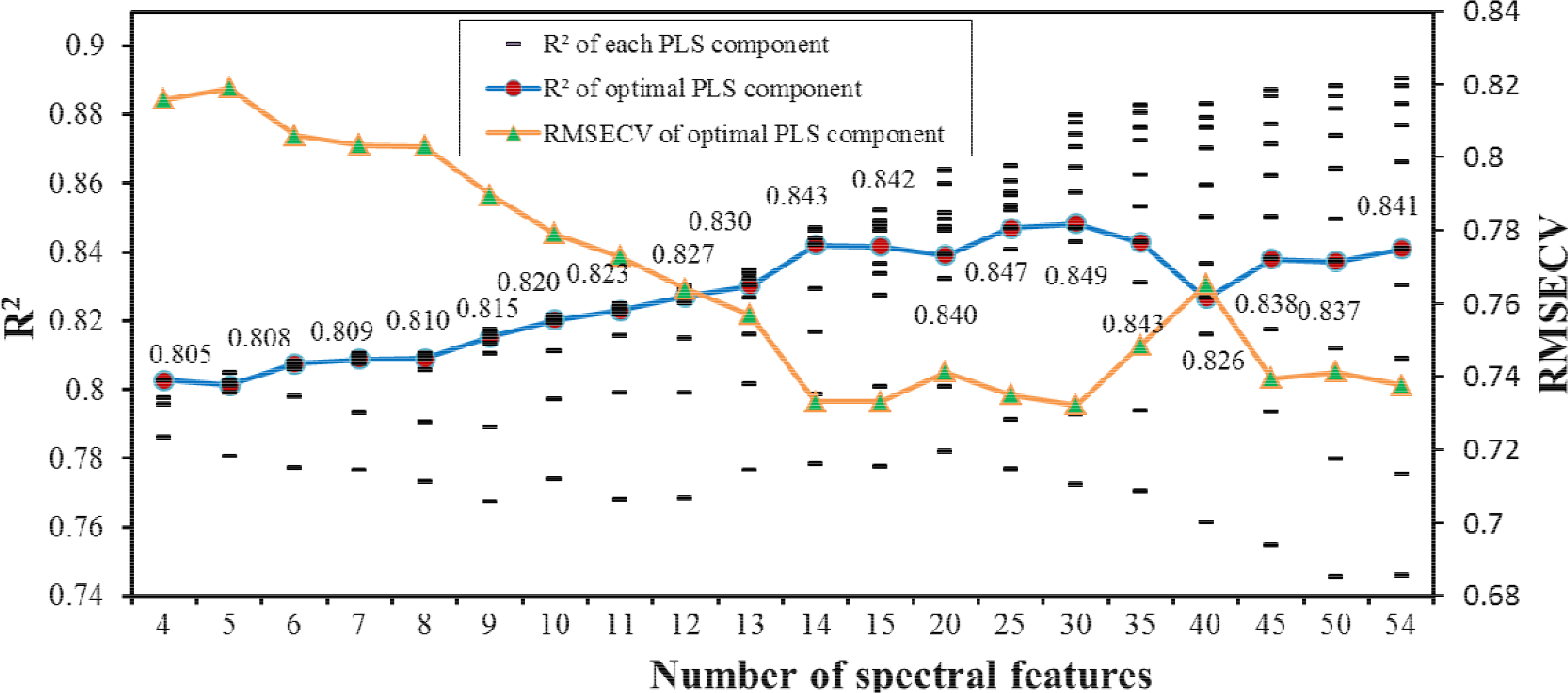
24]. Although the parameter number of the optimal spectral waveband dataset was double that of the optimal spectral position dataset, the prediction accuracy of the 10-variable optimal position feature model performed better than that of the 20-variable optimal waveband feature model. Indeed, the all-feature (54 variables) dataset yielded a lower level of accuracy than the top 30 variables dataset. The results therefore indicate that the continuous addition of variables may not always improve LAI estimation accuracy. Indeed, the inclusion of an increasing number of less important spectral features in PLSR models can negatively influence prediction accuracy [
22,
26].
The calculated VIP scores provided an insight into the usefulness of each variable in the PLS model. The spectral dataset containing the top 14 variables was able to achieve a high level of estimation accuracy with the use of fewer spectral features; the subsequent inclusion of additional features resulted in only a minor improvement in model accuracy. These 14 features included the red-edge region (FD3), the NIR region (FD5, FD6, FD4, FD8, A_Area
2, A_Area
3, R_Area
2 and R_Area
3) and the best vegetation indices (RVI, CI
Red-dege, MSR, MNLI and MTVI2); these were also the best features in the three datasets employed for LAI estimation discussed above. The presented results demonstrate the potential of PLSR and VIP techniques in identifying important variables for the estimation of LAI. It is important to select appropriate features and to determine the optimal variable number(s). Selecting only the very best features selected by VIP values may therefore be sufficient in terms of exploring the rich information available for LAI estimation, with the use of whole feature and/or full spectrum datasets being unnecessary. This finding is in agreement with that of [
25], who identified the most significant indices (chosen via VIP) producing the best PLS model prediction of
T. peregrinus damage.
5. Conclusions
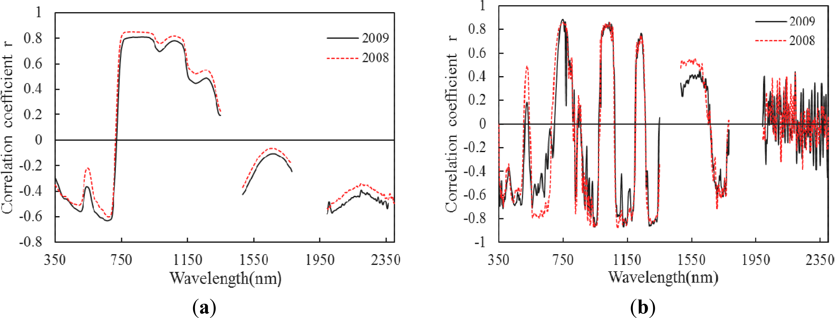
In order to select suitable spectral features for LAI estimation, different features based on spectral wavebands, spectral positions and vegetation indices were evaluated, with all exhibiting the same changing tendency in two years of hyperspectral data. The best features in three different spectral feature groups exhibited a similar correlation with LAI. Derivative analysis, a combination of vegetation index, as well as absorption and reflectance position features generally proved to be better predictors of LAI variability. Spectral features in the red-edge and NIR regions were the most sensitive for predicting LAI. The first derivative at a wavelength of 750 nm exhibited the highest correlation with LAI for all features.
PLSR and VIP analyses were conducted on spectral feature data to estimate LAI and to identify the subset of features with the best predictive accuracy. Our findings suggest that LAI estimation accuracy could be improved by employing the most sensitive spectral features in conjunction with PLSR models. The application of these methods made it possible to extract sufficient signals covering the full spectral range of information, reducing the dimensionality of the hyperspectral data and improving the steady estimation accuracy of winter wheat LAI. The 14 features with the highest VIP values provided a higher level of accuracy in predicting LAI than the entire 54-feature dataset. The validation of the new model indicated that the best feature model performed the best with the mean R2 of 0.880 and the mean RMSE of 0.943.
Compared to other multivariate statistical models, such as principal component regression (PCR) and stepwise multiple linear regression (SMLR), PLSR outperformed other techniques in estimating canopy chlorophyll content, vegetation water content, nitrogen content, LAI, and so on [
24,
67,
68]. However, some methods, such as support vector machines (SVM) and artificial neural networks (ANNs), are also useful for nonlinear models and vegetation canopy property estimations. To evaluate applications of these features and models proposed in this study, other vegetation types and the radiative transfer model approach will be conducted.

 and
and 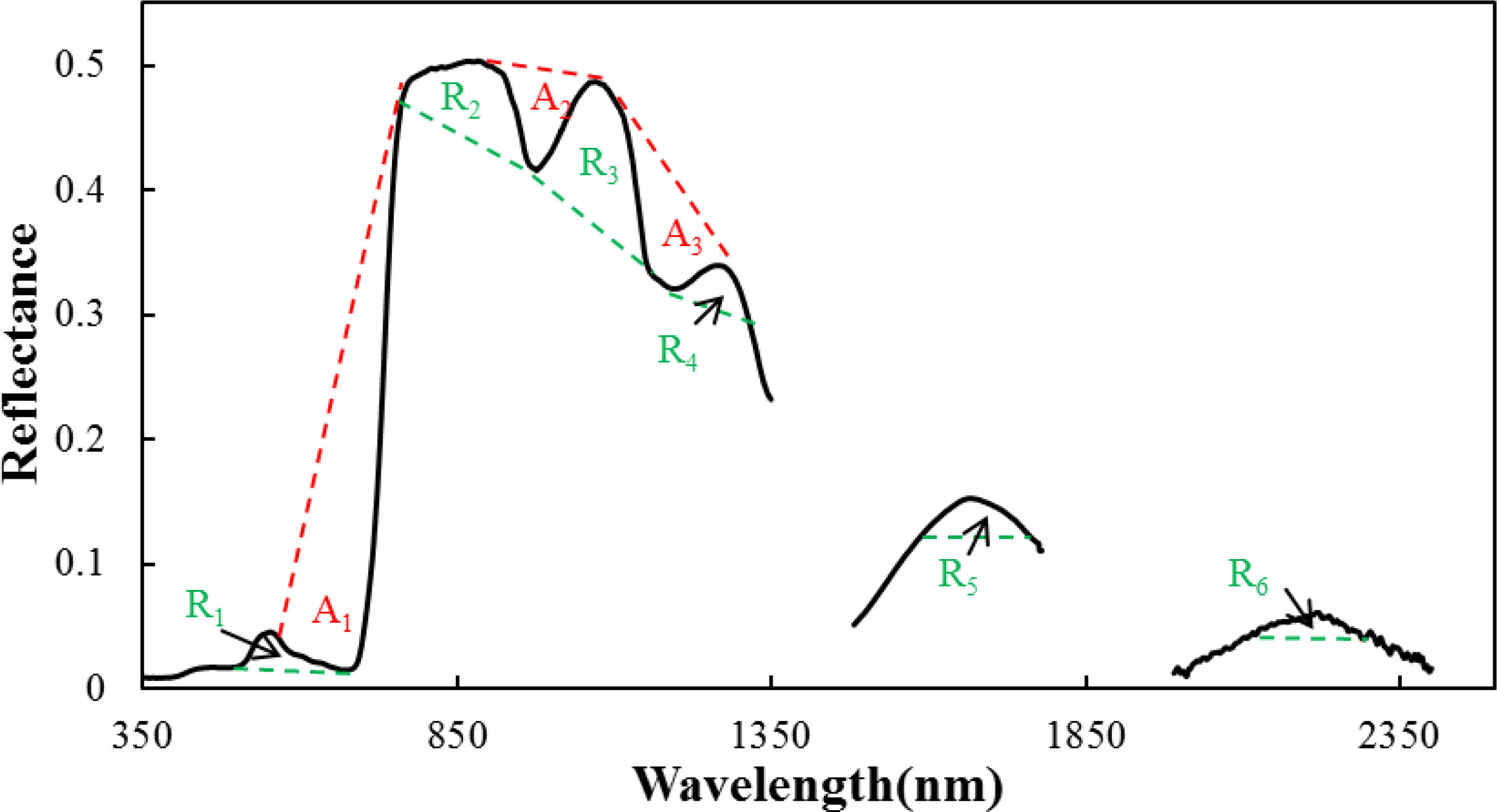


