On the Atmospheric Correction of Antarctic Airborne Hyperspectral Data

Abstract
: The first airborne hyperspectral campaign in the Antarctic Peninsula region was carried out by the British Antarctic Survey and partners in February 2011. This paper presents an insight into the applicability of currently available radiative transfer modelling and atmospheric correction techniques for processing airborne hyperspectral data in this unique coastal Antarctic environment. Results from the Atmospheric and Topographic Correction version 4 (ATCOR-4) package reveal absolute reflectance values somewhat in line with laboratory measured spectra, with Root Mean Square Error (RMSE) values of 5% in the visible near infrared (0.4–1 μm) and 8% in the shortwave infrared (1–2.5 μm). Residual noise remains present due to the absorption by atmospheric gases and aerosols, but certain parts of the spectrum match laboratory measured features very well. This study demonstrates that commercially available packages for carrying out atmospheric correction are capable of correcting airborne hyperspectral data in the challenging environment present in Antarctica. However, it is anticipated that future results from atmospheric correction could be improved by measuring in situ atmospheric data to generate atmospheric profiles and aerosol models, or with the use of multiple ground targets for calibration and validation.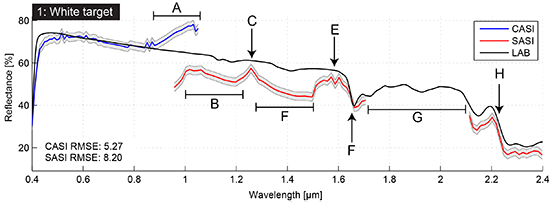
1. Introduction
Antarctica is a unique and geographically remote environment. Field campaigns in the region encounter numerous challenges including the harsh polar climate, steep topography, and high infrastructure costs. Additionally, field campaigns are often limited in terms of spatial and temporal resolution, and particularly, the topographical challenges presented in the Antarctic mean that many areas remain inaccessible. For example, despite more than 50 years of geological mapping on the Antarctic Peninsula, there are still large gaps in coverage, owing to the difficulties in undertaking geological mapping in such an environment [1]. Hyperspectral imaging may provide a solution to overcome the difficulties associated with field mapping in the Antarctic.
Hyperspectral sensors acquire data from a contiguous spectrum over a defined wavelength interval, which makes it possible to identify surface materials by their characteristic reflectance or emittance spectrum, and can yield information on features such as abundance and composition, including ion substitution in minerals [2,3]. It is possible to produce maps of mineral composition and abundance from hyperspectral imagery without rigorous ground truth measurements, due to the development of spectral reflectance libraries (e.g., [4]). A variety of software packages are capable of applying advanced image processing algorithms to hyperspectral imagery using such spectral reflectance libraries, and thus allowing the end-user to produce mineral maps with relative ease. A comprehensive review of geologic remote sensing, including the use of hyperspectral data, is given by van der Meer et al. [5].
The reflectance spectrum of a material can, in principle, be recovered from the observed radiance spectrum over regions in which the illumination is non-zero [6]. The reflectance spectrum is independent of the illumination and provides the best opportunity to identify materials by comparison with reference libraries [6]. In the case of solar illumination (i.e., irradiance from the sun), many environmental and atmospheric effects complicate the process of deconvolving reflectance spectra from the measured radiance, and complex radiative transfer models are required [6]. These models usually simulate the incoming solar irradiance, subsequent atmospheric effects and the final at-sensor radiance; the effects of the intervening atmosphere on the solar irradiation can then be accounted for and reflectance spectra derived. The accurate removal of atmospheric absorption and scattering is required to produce measures of surface reflectance; a process known as atmospheric correction [7]. Atmospheric correction is a common preprocessing step and use of an appropriate, thorough correction is of great significance for interpretation of hyperspectral imagery and any subsequent processing such as classification [8]. A variety of tools exist to perform atmospheric correction with radiative transfer models now mature enough to be used as a routine part of hyperspectral image processing; a comprehensive review of atmospheric correction techniques, including techniques based on radiative transfer, is presented in [7].
In the early 1990s, the Atmosphere Removal Algorithm (ATREM) [9] was developed to employ radiative transfer equations and produce atmospherically corrected spectral data. Since the development of ATREM, several packages have also been developed for atmospherically correcting multi- and hyperspectral data, including High-accuracy ATmospheric Correction for Hyperspectral Data (HATCH) [10], Fast Line-of-Sight Atmospheric Analysis of Spectral Hypercubes (FLAASH) [11,12] and a series of Atmospheric and Topographic Correction (ATCOR) codes [13,14].
The series of ATCOR codes have been continually updated and developed throughout the 1990s and 2000s, with the latest ATCOR-4 release using a large database containing results of radiative transfer calculations based on the MODTRAN-5 [15] radiative transfer model. Additional techniques for correcting adjacency effects, 3D code for correction of topographic effects and bi-direction reflectance distribution function (BDRF) in addition to haze and low cirrus cloud removal are included [14].
The unique atmospheric conditions present in Antarctica combined with the first known hyperspectral data acquisition afford the opportunity to assess the applicability of standard radiative transfer modelling and atmospheric correction techniques for deriving surface reflectance. Previous studies that have carried out atmospheric correction in Antarctica have used multispectral airborne [16] and multispectral satellite data [1] applying radiative transfer modelling techniques to produce reflectance data. However, atmospheric correction of airborne hyperspectral data has not been investigated (due to the previous unavailability of airborne hyperspectral data). This study presents initial results from an investigation into the applicability of the MODTRAN-5 [15] radiative transfer model and the ATCOR-4 atmospheric correction package [14] for producing atmospherically corrected airborne hyperspectral data in the unique Antarctic environment.
2. Study Area
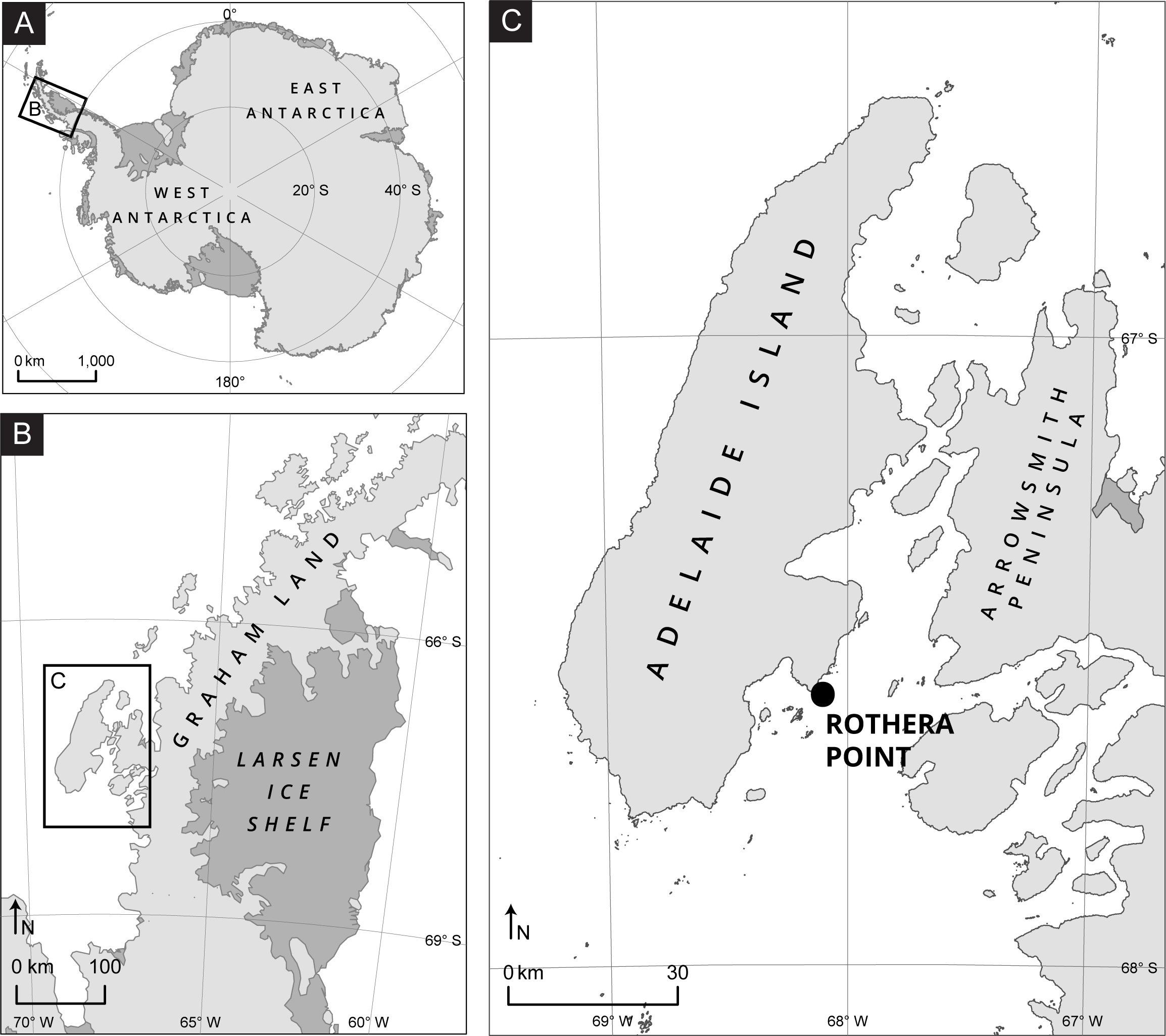
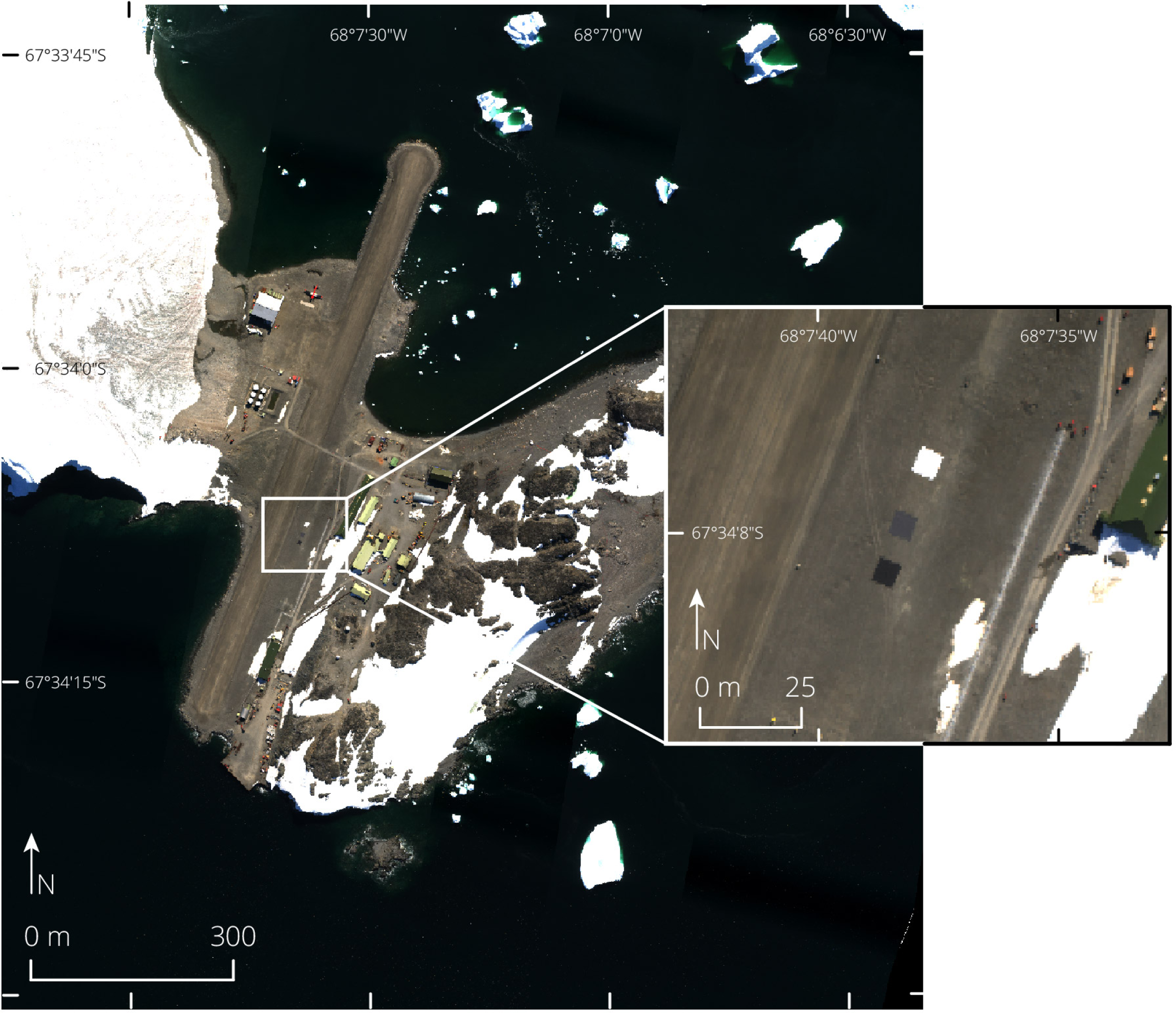
Rothera Point (Figure 1) was surveyed in February 2011, using the ITRES (ITRES Research Ltd., 110, 3553-31st Street NW, Calgary, AB, T2L 2K7, Canada) CASI-1500 and SASI-600 instruments acquiring data in the visible near-infrared (VNIR; 0.4–1.0 μm) and shortwave infrared (SWIR; 1–2.5 μm) portions of the electromagnetic spectrum. Sensor information is presented in Table 1. The acquisition system hardware and other equipment were installed into a British Antarctic Survey (BAS) DeHavilland Twin Otter aircraft. The imagers were installed onto a single mounting plate for concurrent imaging. This arrangement allowed for uniform recording of all aspects of aircraft motion relative to the two imagers with respect to the Inertial Measurement Unit (IMU). The Instrument Control Units (ICUs) were installed at the fore section of the aircraft. Six flight lines were required to acquire hyperspectral data of the study area, and during the acquisition of the imagery, three large (6 m × 6 m) calibration targets were placed within the study area; white, grey and black targets, provided by the Natural Environment Research Council (NERC) Field Spectroscopy Facility [17].
The spectral reflectance measurements of these calibration targets were acquired using an Analytical Spectral Devices (ASD) FieldSpec® Pro, which records continuous spectra across the 350–2500 nm wavelength region; the spectral resolution of the instrument was 3 nm at 700 nm, 10 nm at 1400 nm, and 12 nm at 2100 nm. Reflectance spectra were acquired in “White Reference” mode using a white Spectralon® panel as the reference target, measured at a nadir viewing angle with illumination provided by a tungsten halogen lamp at a 45° angle. Figure 2 shows a colour composite image of Rothera point showing the calibration targets.
3. Methods
3.1. Data Preprocessing
Standard preprocessing of hyperspectral data was carried out by ITRES to produce georeferenced and radiometrically corrected imagery. There are two major steps: Radiometric Correction and Geometric Correction, which were both carried out by ITRES’ propriety tools. In the first step, radiometric and spectral calibration coefficients are applied to convert the raw digital numbers into spectral radiance values. Geometric correction utilizes measurements from the IMU and GPS to create a georeferenced mosaic image.
3.1.1. Radiometric Correction
The raw data are digitized at 14-bit resolution and are recorded as digital numbers (DN). The radiometric processing converted these digital numbers into spectral radiance values based upon calibration coefficient files, which were generated during laboratory calibration of the sensors. Due to the extreme operating conditions during acquisition (very cold temperatures), the image sensors were pushed to their limits and some anomalies were apparent in the image data, particularly in the SASI images. The SASI instrument’s operating conditions were significantly different to the calibration conditions in the laboratory, hence scaling and spectral resampling adjustments, ranging from −5% to +10%, were made to the calibration files to compensate for these environment effects and minimise the anomalies introduced as a result of the operating conditions.
3.1.2. Geometric Correction
After radiometric correction, the data was geometrically calibrated. The ITRES proprietary geometric correction software utilised the navigation solution, bundle adjustment parameters and Digital Elevation Models (DEMs) to produce georeferenced radiance image files for each flight line. In addition, flight lines were combined into an image mosaic of the area. The nearest neighbour algorithm was used to populate the image pixels so that radiometric integrity of the pixels could be preserved. At the image mosaicking stage, a minimised nadir angle approach was implemented such that the spectra of the pixel with the smallest off-nadir angle from overlapping adjacent flight lines was written to the final mosaic image.
3.1.3. Radiance Offset
The spectral range of the CASI and SASI data (Table 1) has an approximate 100 nm overlap, between 950 nm and 1055.5 nm. Preliminary investigations revealed an offset in radiance values within this overlap range. In the overlap range, CASI radiance values were found to be larger than the corresponding SASI radiance, with a trend of increasing radiance offset with increasing wavelength. This radiance offset is present in the radiometrically calibrated data. Several factors are likely to have produced the radiance offset.
The first and most probable contributing factor is second order light contributions. The CASI sensor’s diffraction grating produces a second order diffraction spectrum, whose blue end overlaps with the red- near infrared (NIR) end of the first order spectrum. Illumination conditions at the time of acquisition may have allowed this effect to lead to additive background signal at the red-NIR end. The second contributing factor could be the reduced calibration accuracy in the NIR end of the spectrum, as the CASI sensor is less sensitive at the longest wavelengths.
Thirdly, preliminary investigations also revealed a systematic underestimation of radiance values in the SWIR (from the SASI instrument). This is attributed to the conditions during acquisition. The instruments were operating in an unpressurised aircraft, with temperatures significantly outside the normal operational range; the SASI instrument was as much as 20 °C (68 °F) outside its normal operating range. These conditions meant there was a noticeable degradation in the response of the sensor, and hence the measured at-sensor radiance was lower in the SWIR data.
3.2. Atmospheric Correction
The Antarctic has a distinct atmosphere, dominated by cold temperatures and unusual light conditions [18]. The atmosphere has stable stratification in the boundary layer, and is pristine, dry and isolated from the rest of the world’s atmosphere by the polar vortex and the Southern Ocean [18]. To produce atmospherically corrected data, ATCOR-4 was used.
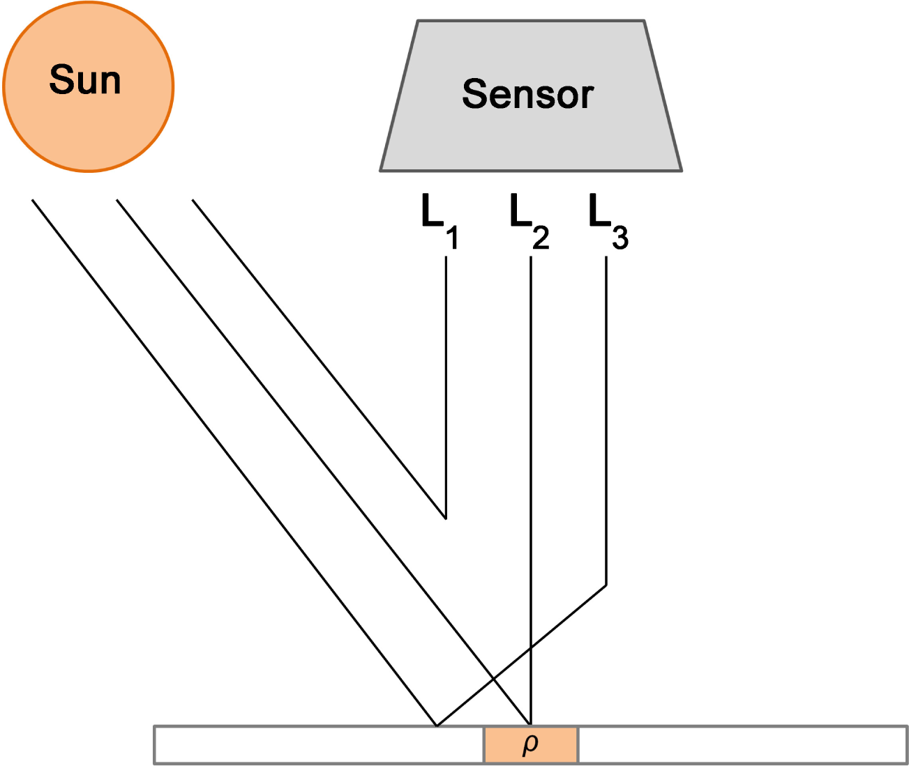
The at-sensor signal consists of three main components, as shown in Figure 3: scattered or path radiance L1, reflectance radiance from the pixel under consideration L2, and radiation reflected from the neighbourhood into the viewing direction (adjacency effect) L3. Component L2 is the only component that contains information on the surface properties of the pixel under consideration, therefore atmospheric correction aims to remove the L1 and L3 components. The atmospheric correction has to be performed iteratively to derive surface reflectance, ρ, for each pixel in the image data. The implementation is described in detail in Chapters 2 and 10 of [19] and in [14].
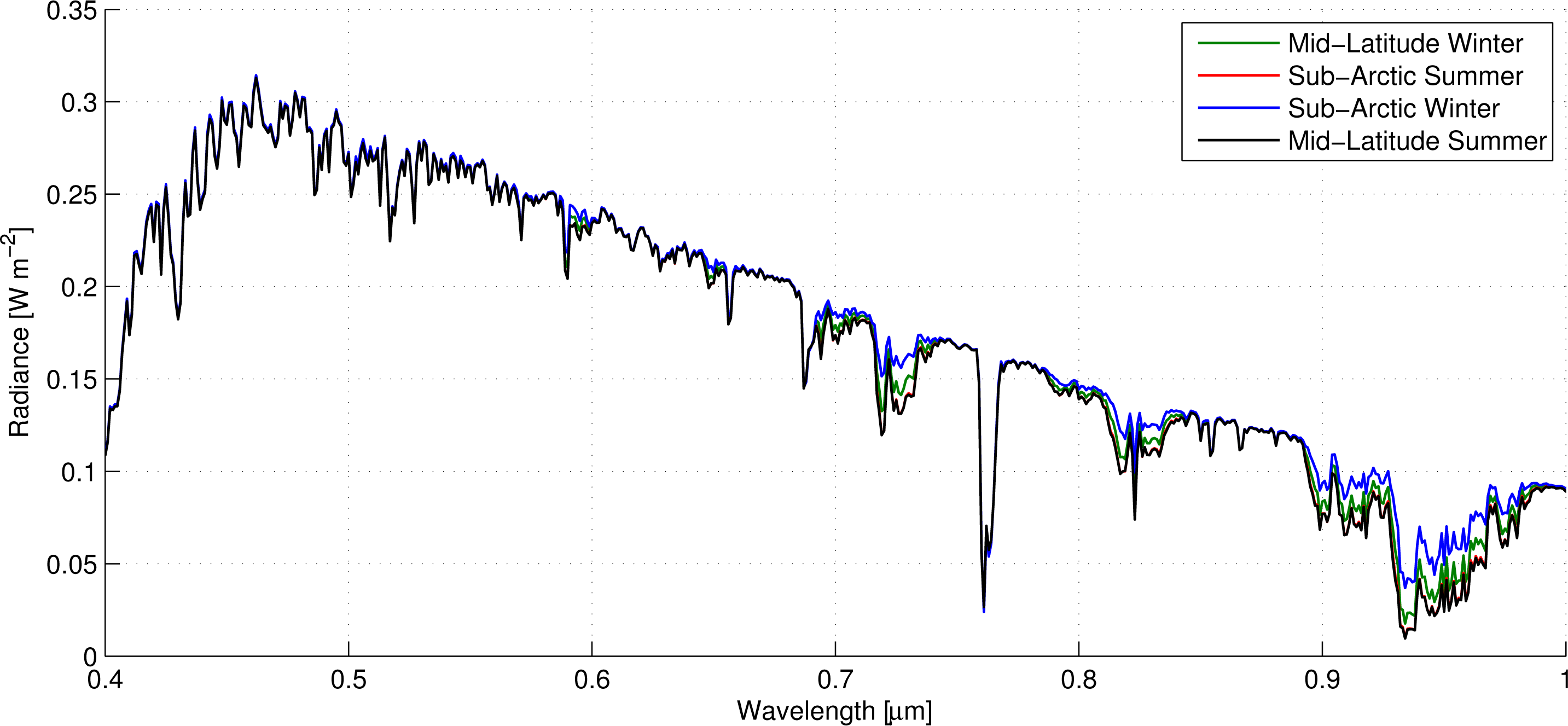
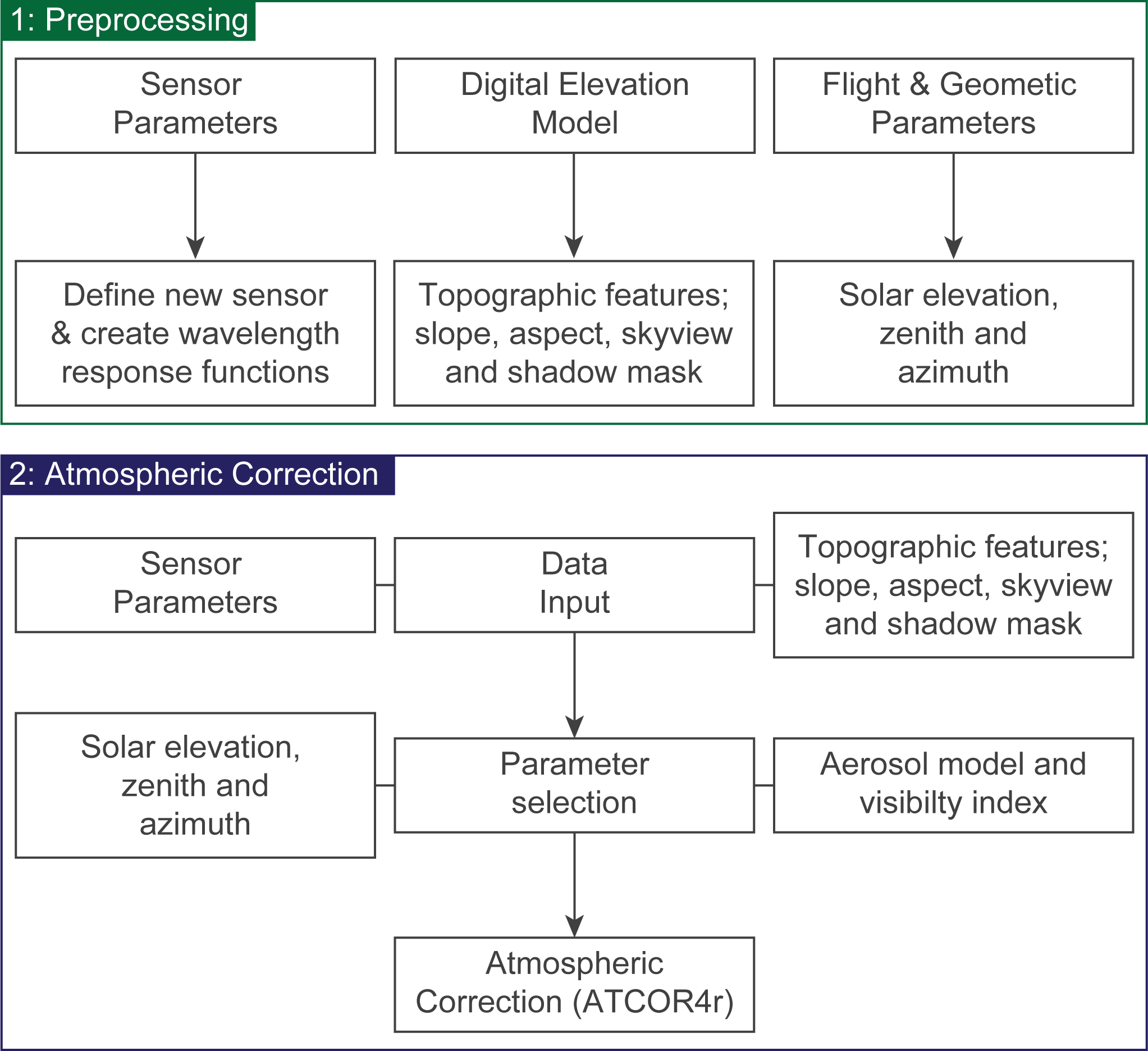
The MODTRAN-5 [15] radiative transfer model is used to generate Look-Up Tables (LUTs) that are used by ATCOR-4 to aid in the calculation of the Ln terms and the subsequent derivation of surface reflectance, ρ. The LUTs utilised by ATCOR-4 require significant computational effort to compute and are based on the “Mid-Latitude Summer” (MLS) profile [20]. LUTs are calculated using MODTRAN-5 with the scaled discrete ordinate radiance transfer (DISORT) option in regions where scattering is dominant and the more accurate correlated-k option in regions where absorption is dominant ([19], p. 154). ATCOR-4’s LUTs were generated using the MLS profile and fixed water vapour contents of 0.4, 1, 2, 2.9, and 4 g/cm2 (rather than the water vapour defined in the standard MLS model [20]). Water vapour is the main parameter that produces differences in radiance values and the other parameters are mostly stable [21]. This can be confirmed by simulating radiance values with each of the atmospheric profiles from [20] and fixed water vapour values in MODTRAN (cf. Figure 4). Full details of the algorithms applied by ATCOR-4 are detailed in [14,19]. The major processing phases of ATCOR-4 are outlined in Figure 5, “Preprocessing” and “Atmospheric Correction”.
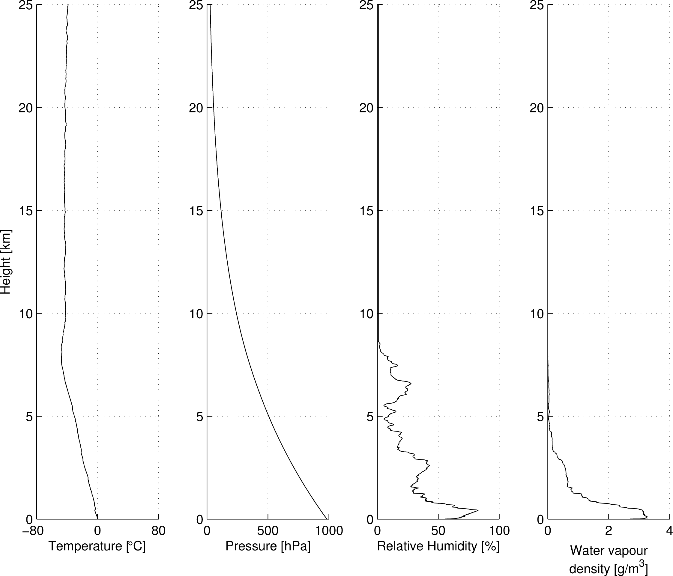
Standard input parameters (location, date and time) were used (Table 2). The other user-selectable parameters are the visibility, choice of aerosol model and choice of water vapour LUT. The visibility is measured hourly by the meteorologists at Rothera Point and the observation closest to data acquisition time was used. The maritime aerosol, interpolated to the flying height, was selected. Coincident meteorology data measured from a radiosonde launch at Rothera Point is shown in Figure 6 indicating the atmospheric conditions close to the time of image acquisition. Additionally, as implied by the measured visibility (60 km), the operators’ notes indicated that the “flight conditions were clear and calm, with blue skies and a few scattered clouds”. With regards to water vapour, the LUT with a water vapour value of 2.0 g/cm2 was selected. However, the choice of water vapour value is not significant because during processing water vapour is recalculated per-pixel; both the CASI-1500 and SASI-600 sensors have bands that lie within water vapour regions and thus the water vapour can be calculated from the image data (see Chapter 10.4.3 in [19] for further details on the water vapour retrieval algorithm).
4. Results
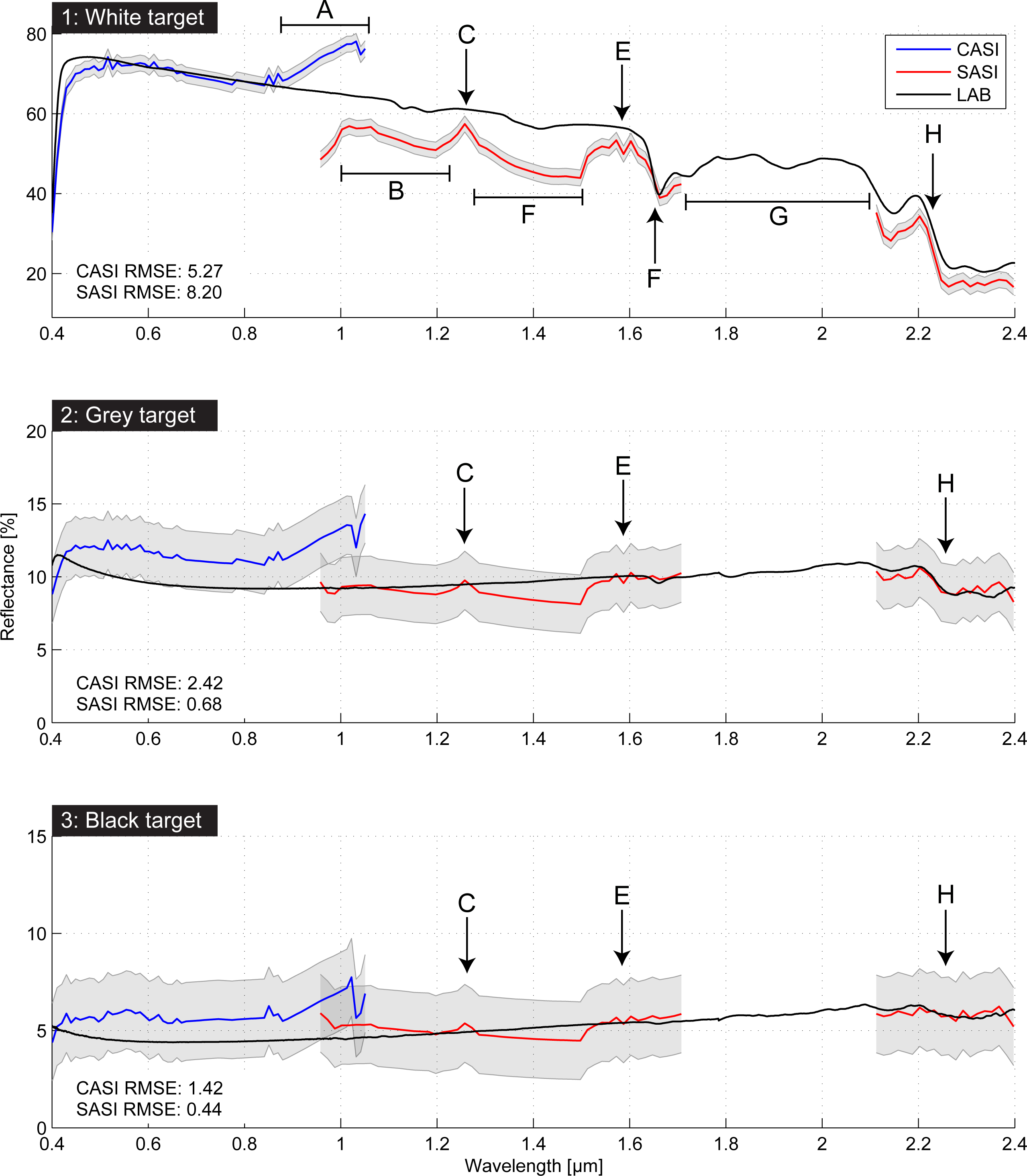
The atmospheric correction results for each of the calibrated targets are presented in Figure 7. For the CASI data, there is a systematic overestimation in reflectance data for the grey and black targets. Between ∼0.86 μm and 1.1 μm there is a noticeable increase in reflectance (A) for the CASI data. This significant increase at the red–NIR end of the spectral range is likely a result of the second order light contribution from the blue end of the spectrum, resulting in additive background signal in the red–NIR end, therefore causing an increase in reflectance values. The SASI data shows a large systematic underestimation for the white target, but less so for the grey and black targets where results are close to or within the ±2% error margins.
Numerous artefacts remain in the CASI and SASI data, most likely as a result of atmospheric gases and aerosols. The residual effects of water vapour (H2O) are most noticeable; interpolation is carried out during the ATCOR-4 processing chain across areas of H2O absorption from 1.0 μm to 1.2 μm (B), leaving a peak at 1.25 μm (C) and a secondary area of interpolation from ∼1.3 μm to 1.5 μm (D). A double peak is present at 1.6 μm due to CO2 absorption (E). The absence of data between 1.7 μm and 2.1 μm (G) is due to the absorption by H2O and CO2, which reduces radiance transmission to almost zero in this portion of the spectrum. There are also some other minor artefacts, such as a double peak at 0.5 μm as a result of O3 and a small peak at ∼0.85 μm likely a result of O2.
In spite of these imperfections, two closely matched absorption features in the targets are found, the first at ∼1.65 μm (F) and the second at ∼2.2 μm (H).
5. Accuracies, Errors and Uncertainties
As discussed in Section 2, the instruments used for data acquisition were flown in an unpressurised BAS DeHavilland Twin Otter aircraft. This meant the instruments were subject to extreme changes in temperature between data acquisition and storage of the instruments in between flights, along with very cold operating conditions during data acquisition itself (up to 20 °C (68 °F) outside of the instrument’s normal operating range). It was identified during the preprocessing of the data (Section 3.1) that the SASI instrument particularly suffered as a result of the heating and cooling cycles and the cold operating conditions it underwent during the data collection campaign in the Antarctic. As a result, during the radiometric correction of the SASI data (Section 3.1.1.) larger adjustments were made to the calibration parameters to correct for the operating conditions in the Antarctic. This introduced some uncertainty in the data, which was observed in the raw data (Section 3.1.3.) and is manifested in the atmospheric correction results (Section 4 and Figure 7) where the SASI data shows a systematic underestimation in reflectance values.
Following atmospheric correction, Root Mean Square Error (RMSE) values were calculated and are annotated on Figure 7. RMSE values were calculated from the ATCOR-4 results with respect to the laboratory measured spectra using Equation (1):
The atmospheric correction approach presented here is subject to uncertainties introduced through the application of the MODTRAN-5 standard atmospheric profiles and aerosol models [20,22]. Namely, these climatologically developed profiles are assumed to represent the true atmospheric conditions at the time of data acquisition. Radiosonde measurements were acquired from the same day (Figure 6), but there was a 4 hour difference between the radiosonde launch (11:38 UTC) and data acquisition (∼15:30 UTC). The variability and local scale differences in the atmosphere (e.g., [23]) mean that, even over this relatively short time scale, applying the measured atmospheric parameters from the radiosonde launch would not necessarily be any more valid than applying the atmospheric profile from the MODTRAN-5 model; both methods are applying a profile with the assumption that it represents the true atmosphere at the time of data acquisition, thereby introducing uncertainty in the results.
These uncertainties could be removed by measuring the actual in situ atmospheric conditions using other instruments simultaneously whilst acquiring the image data. However, in this study, as is the case in most other studies applying similar techniques, simultaneous atmospheric measurements are unavailable. Despite making assumptions about atmospheric profiles and introducing uncertainties, the radiative transfer model and atmospheric correction approach has been applied successfully. As long as appropriate error metrics are calculated (e.g., RMSE) and the data is carefully applied in additional processing (e.g., spectral mapping) then these uncertainties can be managed and minimised throughout the entire processing chain.
6. Discussion
The atmospheric correction processing chain and results presented here represent the first known acquisition and subsequent processing of hyperspectral data in Antarctica. The presence of ground targets along with concurrent ground and atmospheric measurements in this study is typical of most hyperspectral campaigns; often there are not sufficient measurements to fully develop atmospheric profiles and aerosol models (to use as inputs to radiative transfer models), hence estimates are made and often standard atmospheric profiles and aerosol profiles are selected based on qualitative assessment of environmental conditions. Additionally, there are not always a large enough number of ground-based targets with the relevant concurrent spectral data to be used for both calibration and validation. The MODTRAN-5 LUTs used by ATCOR-4 were intended to be flexible enough to cover a wide variety of environments, sensor configurations, water vapour contents and flight parameters but have not been previously tested for airborne hyperspectral data in the Antarctic region.
Following the application of the atmospheric correction processing chain, the results showed that workable reflectance data is obtainable. This is obtainable in spite of limited concurrent atmospheric and aerosol measurements combined with assumptions about aerosol model parameters (for example, the maritime aerosol model was selected based on qualitative interpretations of the Antarctic environment), which is an often typical scenario. As there are no aerosol measurements collected at Rothera, the maritime aerosol model [22] was selected based on the qualitative assessment of the atmospheric conditions and the assumption of a dominance of sea salt aerosols in the coastal Antarctic environment (e.g., compare [24]). For the lower reflectance targets (<20%), the results from the both VNIR (CASI-1500) and SWIR (SASI-600) sensors fell within the expected ±2% margins; however, this is likely an artefact of the low signal-to-noise ratio (<15:1) for low reflectance targets. The higher reflectance target (the white target) shows clear discrepancies, with absolute reflectance values differing by as much as 30%. The white target is perhaps more representative of the overall performance of the atmospheric correction due to its higher signal-to-noise ratio.
Despite the discrepancies between absolute reflectance values, absorption features for the white target (e.g., 1.65 μm and 2.25 μm) are clearly discerned; similar absorption features in the lower reflectance (grey and black) targets also correlate well between the laboratory-measured and atmospherically corrected reflectance data. There is still residual noise manifested as small peaks and spikes in the reflectance data, which could complicate post-processing procedures, particularly those that rely on relative differences between peaks and troughs in spectra. The residual noise manifested in peaks and spikes are most likely due to the unavailability of an Antarctic-specific atmospheric profile and aerosol model, due the lack of adequate in situ measurements. Additionally, portions of the spectrum that are strongly affected by water vapour (e.g., the interpolation from 1.3 μm to 1.5 μm, and the lack of data between 1.7 μm and 2.1 μm) prove difficult to characterise; a finding that supports the conclusions of Zibordi and Maracci [16] who noted that uncertainties in calculating water vapour optical thickness could lead to “very significant error” ([16], p. 20).
These results suggest that commercially available atmospheric correction packages are flexible enough to produce working reflectance data in Antarctica. Performance is poorer with higher reflectance targets, though results fall within the expected error margins for lower reflectance targets. The ability to discriminate absorption features suggests that the atmospheric correction process would produce reflectance data capable of being applied in mapping techniques using absorption features (e.g., continuum removal). Particular care would have to be given when working with absolute reflectance values.
It is recommended that, given the availability of a greater number of ground targets (>3), a hybrid approach of radiative transfer modelling followed by the Empirical Line Method (ELM) [25] be applied for potentially improved results; for example Tuominen and Lipping [26] reported a reduction in Root Mean Square Error (RMSE) from 6.8% to 1.8% when combining the hybrid approach of radiative transfer modelling through ATCOR-4 and the ELM, compared with radiative transfer modelling alone. Therefore, following the conclusions of Tuominen and Lipping [26], it can be seen that even in complex atmospheres where model-based correction methods may struggle, more accurate results can be produced using combined correction methods compared with model- or empirical-based methods alone. It was also noted that even in situations when there is a limited number of spectral ground truth measurements, a hybrid approach can improve atmospheric correction accuracy over the whole acquisition area [26].
This approach was successfully applied to Advanced Spaceborne Thermal Emission and Reflection Radiometer (ASTER) VNIR/SWIR data by Haselwimmer et al. [1], who utilised the hybrid approach combining the FLAASH radiative transfer model [11,12] and an empirical correction. Haselwimmer et al. [1] utilised spectral measurements of the runway at Rothera Point assuming that the runway is a Pseudo-Invariant Feature (PIF) [27,28]. PIFs are large uniform targets whose spectral reflectance is assumed not to have changed over time [28]. In cases where appropriate PIFs have been identified and measured, they can provide a suitable ground truth feature for calibration or validation. PIFs can be used either as a substitute for or in conjunction with calibrated targets (such as those used in this study) to provide enough targets (>3) for the hybrid approach of radiative transfer modelling followed by empirical line correction. The identification of suitable PIFs in the Antarctic generally, and particularly in the regions where the airborne hyperspectral data was acquired, remains an area of on-going investigation. If a suitable number of targets are identified, the need for deploying calibrated targets during image acquisition may be negated, as PIFs may allow for both calibration and validation of atmospheric correction methods.
It must also be noted that sensor calibration still remains challenging in this environment and these issues are manifested in the subsequent atmospheric correction process. Particularly notable effects of this can be observed in Figure 7, such as the offset between VNIR and SWIR (CASI and SASI) sensor values in the overlapping region (0.95 μm to 1.05 μm), as well as the significant underestimation of reflectance for the white target for the SWIR (SASI) data.
Future studies should consider the influence of radiative transfer models’ standard atmospheric profiles [20] and aerosol model types [22] with a view to measuring in situ atmospheric data while simultaneously acquiring hyperspectral data; this would aid in the generation of atmospheric profiles and aerosol models that serve as inputs during the atmospheric correction process and reduce the level of uncertainty when assumed profiles are used. Such atmospheric data could also lead to the development of a generic “Antarctic” atmospheric profile and aerosol model, which may prove useful for future data acquisition (where measuring in situ atmospheric data is not possible).
7. Conclusions
This study has presented results from atmospheric correction of airborne hyperspectral data in Antarctica. The findings are significant as they represent (a) the first known acquisition and preprocessing of airborne hyperspectral data in Antarctica, and (b) the first assessment of atmospheric correction techniques applied to airborne hyperspectral data in Antarctica. The atmospheric correction technique utilised a radiative transfer model (MODTRAN-5) [15] in the Atmospheric and Topographic Correction version 4 package (ATCOR-4) [14].
Two sensors, imaging the visible near-infrared (VNIR; 0.4–1.0 μm) and shortwave infrared (SWIR; 1–2.5 μm), were deployed during the data acquisition. During the radiometric correction (preprocessing) of the data it was found that, as a result of the extreme temperature variations during the data collection, the SWIR sensor had decreased sensitivity, resulting in lower measured radiance values and systematic underestimation in reflectance values following atmospheric correction. The results from atmospheric correction revealed that obtaining surface reflectance of airborne hyperspectral data in the Antarctic is possible without in situ measurements of atmospheric parameters; reflectance data had maximal Root Mean Square Error (RMSE) values of 5% in the VNIR and 8% in the SWIR. However, residual noise remains present in the reflectance data as a result of using standard atmospheric profiles and aerosol models during the atmospheric correction process.
For future campaigns in Antarctica, it is recommended that instruments be sufficiently tested and calibrated to operate successfully in cold environments, with particular attention given to imagers operating in the SWIR. During acquisition it is recommended that (a) in situ atmospheric data be measured simultaneously whilst acquiring hyperspectral data to produce robust atmospheric and aerosol profiles that can be applied during the atmospheric correction process, and (b) ground truth data, such as calibrated targets or pseudo-invariant features, be present to allow for the validation of atmospheric correction results, as well as calibration of reflectance data using empirical correction techniques (if a sufficient number of ground targets allow, i.e., >3).
Acknowledgments
The Hyperspectral Data used was collected during an airborne survey funded by the UK Foreign and Commonwealth Office (FCO) and conducted by the British Antarctic Survey, ITRES Research Ltd. and Defence Research & Development Suffield, Canada in February 2011. Loans for the calibrated targets and associated laboratory spectra were provided by the Natural Environment Research Council (NERC) Field Spectroscopy Facility. MB is funded by a Natural Environment Research Council (NERC) PhD studentship in conjunction with the British Antarctic Survey and the University of Hull (NERC Grant: NE/K50094X/1). Anonymous reviewers are thanked for their comments on earlier versions of the manuscript.
Author Contributions
Martin Black is the main author who performed the atmospheric correction and wrote the draft version of the manuscript. Andrew Fleming, Stephen Achal and John McFee were involved in the data acquisition. Stephen Achal and Alejendra Umana Diaz were responsible for the data preprocessing. Andrew Fleming, Peter Fretwell, Graham Ferrier and Teal Riley supervised and participated with the work throughout all phases. All authors provided assistance in writing, editing and organising the manuscript.
Conflicts of Interest
The authors declare no conflicts of interest.
References
- Haselwimmer, C.E.; Riley, T.R.; Liu, J.G. Assessing the potential of multispectral remote sensing for lithological mapping on the Antarctic Peninsula: Case study from eastern Adelaide Island, Graham Land. Antarct. Sci 2010, 22, 299–318. [Google Scholar]
- Clark, R.N. Spectroscopy of Rocks and Minerals, and Principles of Spectroscopy. In Manual of Remote Sensing; Rencz, A.N., Ed.; John Wiley and Sons: New York, NY, USA, 1999; pp. 3–58. [Google Scholar]
- Drury, S.A. Image Interpretation in Geology; Blackwell Science: Oxford, UK, 2001; p. 209. [Google Scholar]
- Baldridge, A.; Hook, S.; Grove, C.; Rivera, G. The ASTER spectral library version 2.0. Remote Sens. Environ 2009, 113, 711–715. [Google Scholar]
- Van der Meer, F.D.; van der Werff, H.M.; van Ruitenbeek, F.J.; Hecker, C.A.; Bakker, W.H.; Noomen, M.F.; van der Meijde, M.; Carranza, E.J.M.; de Smeth, J.B.; Woldai, T. Multi- and hyperspectral geologic remote sensing: A review. Int. J. Appl. Earth Obs. Geoinfor 2012, 14, 112–128. [Google Scholar]
- Shaw, G.A.; Burke, H.H.K. Spectral imaging for remote sensing. Linc. Lab. J 2003, 14, 3–28. [Google Scholar]
- Gao, B.C.; Montes, M.J.; Davis, C.O.; Goetz, A.F. Atmospheric correction algorithms for hyperspectral remote sensing data of land and ocean. Remote Sens. Environ 2009. [Google Scholar] [CrossRef]
- Mahiny, A.S.; Turner, B.J. A comparison of four common atmospheric correction methods. Photogramm. Eng. Remote Sens 2007, 73, 361–368. [Google Scholar]
- Gao, B.C.; Heidebrecht, K.B.; Goetz, A.F. Derivation of scaled surface reflectances from AVIRIS data. Remote Sens. Environ 1993, 44, 165–178. [Google Scholar]
- Qu, Z.; Kindel, B.; Goetz, A.F.H. The High Accuracy Atmospheric Correction for Hyperspectral Data (HATCH) model. IEEE Trans. Geosci. Remote Sens 2003, 41, 1223–1231. [Google Scholar]
- Matthew, M.; Adler-Golden, S.; Berk, A.; Felde, G.; Anderson, G.; Gorodetzky, D.; Paswaters, S.; Shippert, M. Atmospheric Correction of Spectral Imagery: Evaluation of the FLAASH Algorithm with AVIRIS Data. Proceedings of the 31st Applied Imagery Pattern Recognition Workshop, Washington, DC, USA, 16–18 October 2002; pp. 157–163.
- Alder-Golden, S.; Berk, A.; Bernstein, L.S.; Richtsmeier, S.; Acharya, P.K.; Matthew, M.W.; Anderson, G.P.; Allred, C.L.; Jeong, L.S.; Chetwynd, J. H. FLAASH, a MODTRAN4 Atmospheric Correction Package for Hyperspectral Data Retrievals and Simulations. Proceedings of the 7th JPL AVIRIS Airborne Earth Science Workshop, Pasadena, CA, USA, 11–12 January 1998; p. 6.
- Schläpfer, D.; Richter, R. Geo-atmospheric processing of airborne imaging spectrometry data. Part 1: Parametric orthorectification. Int. J. Remote Sens 2002, 23, 2609–2630. [Google Scholar]
- Richter, R.; Schläpfer, D. Geo-atmospheric processing of airborne imaging spectrometry data. Part 2: Atmospheric/topographic correction. Int. J. Remote Sens 2002, 23, 2631–2649. [Google Scholar]
- Berk, A.; Anderson, G.P.; Acharya, P.K.; Bernstein, L.S.; Muratov, L.; Lee, J.; Fox, M.J.; Adler-Golden, S.M.; Chetwynd, J.H.; Hoke, M.L.; et al. MODTRAN5: A reformulated atmospheric band model with auxiliary species and practical multiple scattering options. Proc. SPIE 2005. [Google Scholar] [CrossRef]
- Zibordi, G.; Maracci, G. Reflectance of antarctic surfaces from multispectral radiometers: The correction of atmospheric effects. Remote Sens. Environ 1993, 43, 11–21. [Google Scholar]
- NERC Field Spectroscopy Facility. Available online: http://www.fsf.nerc.ac.uk (accessed on 7 January 2014).
- Simpson, W.R.; von Glasow, R.; Riedel, K.; Anderson, P.; Ariya, P.; Bottenheim, J.; Burrows, J.; Carpenter, L.J.; Frieß, U.; Goodsite, M.E.; et al. Halogens and their role in polar boundary-layer ozone depletion. Atmos. Chem. Phys 2007, 7, 4375–4418. [Google Scholar]
- Richter, R.; Schläpfer, D. Atmospheric/Topographic Correction for Airborne Imagery, ATCOR-4 User Guide, Version 6.2.1. DLR-IB 565-02/08; Deutsches Zentrum für Luft- und Raumfahrt (DLR): Weßling, Germany, 2014; p. 225. [Google Scholar]
- McClatchey, R.A.; Fenn, R.; Selby, J.A.; Volz, F.; Garing, J. Optical Properties of the Atmosphere; Technical Report AFCRL-72-0497; Environmental Research Paper Air Force Geophysics Lab, Optical Physics Division, Hanscom AFB: Boston, MA, USA, 1972. [Google Scholar]
- Schläpfer, D. (ReSe Applications Schläpfer, Langeggweg 3, CH-9500, Wil, Switzerland). Personal communication,. 2013. [Google Scholar]
- Shettle, E.; Fenn, R. Models for the Aerosols of the Lower Atmosphere and the Effects of Humidity Variations on Their Optical Properties; Technical Report AFGL-TR-79-0214; Environmental Research Paper Air Force Geophysics Lab, Optical Physics Division, Hanscom AFB: Boston, MA, USA, 1979. [Google Scholar]
- Harangozo, S.A.; Colwell, S.R.; King, J.C. An analysis of a 34-year air temperature record from Fossil Bluff (71S, 68W), Antarctica. Antarct. Sci 1997, 9, 355–363. [Google Scholar]
- Rankin, A.M.; Wolff, E.W. A year-long record of size-segregated aerosol composition at Halley, Antarctica. J. Geophys. Res.: Atmos 2003, 108, 1–6. [Google Scholar]
- Smith, G.M.; Milton, E.J. The use of the empirical line method to calibrate remotely sensed data to reflectance. Int. J. Remote Sens 1999, 20, 2653–2662. [Google Scholar]
- Tuominen, J.; Lipping, T. Atmospheric Correction of Hyperspectral Data Using Combined Empirical and Model Based Method. Proceedings of the 7th European Association of Remote Sensing Laboratories SIG-Imaging Spectroscopy Workshop, 11–13 April 2011; Edinburgh, Scotland, UK.
- Freemantle, J.; Pu, R.; Miller, J. Calibration of Imaging Spectrometer Data to Reflectance Using Pseudo-Invariant Features. Proceedings of the 15th Canadian Symposium on Remote Sensing, Toronto, ON, Canada, 1–4 June 1992; pp. 1–4.
- Philpot, W.; Ansty, T. Analytical Description of Pseudo-Invariant Features (PIFs). Proceedings of the 6th International Workshop on the Analysis of Multi-temporal Remote Sensing Images (Multi-Temp), Trento, Italy, 12–14 July 2011; pp. 53–56.


| Instrument | Specification |
|---|---|
| CASI-1500 | 1500 across-track imaging pixels |
| 72 spectral bands in 367.6–1055.5 nm | |
| Spectral bandwidth of 9.6 nm | |
| 40° field of view | |
| 0.5 m ground resolution | |
| SASI-600 | 600 across-track imaging pixels |
| 100 spectral bands in 950–2450 nm | |
| Spectral bandwidth of 15 nm | |
| 40° field of view | |
| 1 m ground resolution | |
| Applanix POS/AV 510 | 3-axis SAGEM IMU |
| Integrated dual frequency Trimble GPS receiver | |
| Real-time roll absolute accuracy (RMS): 0.008° | |
| Real-time pitch absolute accuracy (RMS): 0.008° | |
| Real-time heading absolute accuracy (RMS): 0.04° | |
| Parameter | Value |
|---|---|
| Date (DD/MM/YYYY) | 07/02/2011 |
| Time (HH:MM) | 15:28 UTC |
| Solar Zenith (degrees) | 53.8 |
| Solar Azimuth (degrees) | 23.6 |
| Flight Heading (degrees) | 76.1 |
| Flight Altitude (m · AGL) | 596.9 |
| Visibility (km) | 60 |
| Atmospheric profile | MLS (2.0 g/cm2) |
| Aerosol model | Maritime (597 m) [22] |
© 2014 by the authors; licensee MDPI, Basel, Switzerland This article is an open access article distributed under the terms and conditions of the Creative Commons Attribution license (http://creativecommons.org/licenses/by/3.0/).
Share and Cite
Black, M.; Fleming, A.; Riley, T.; Ferrier, G.; Fretwell, P.; McFee, J.; Achal, S.; Diaz, A.U. On the Atmospheric Correction of Antarctic Airborne Hyperspectral Data. Remote Sens. 2014, 6, 4498-4514. https://doi.org/10.3390/rs6054498
Black M, Fleming A, Riley T, Ferrier G, Fretwell P, McFee J, Achal S, Diaz AU. On the Atmospheric Correction of Antarctic Airborne Hyperspectral Data. Remote Sensing. 2014; 6(5):4498-4514. https://doi.org/10.3390/rs6054498
Chicago/Turabian StyleBlack, Martin, Andrew Fleming, Teal Riley, Graham Ferrier, Peter Fretwell, John McFee, Stephen Achal, and Alejandra Umana Diaz. 2014. "On the Atmospheric Correction of Antarctic Airborne Hyperspectral Data" Remote Sensing 6, no. 5: 4498-4514. https://doi.org/10.3390/rs6054498
APA StyleBlack, M., Fleming, A., Riley, T., Ferrier, G., Fretwell, P., McFee, J., Achal, S., & Diaz, A. U. (2014). On the Atmospheric Correction of Antarctic Airborne Hyperspectral Data. Remote Sensing, 6(5), 4498-4514. https://doi.org/10.3390/rs6054498