On Line Validation Exercise (OLIVE): A Web Based Service for the Validation of Medium Resolution Land Products. Application to FAPAR Products


 , ,
, , 

Abstract
: The OLIVE (On Line Interactive Validation Exercise) platform is dedicated to the validation of global biophysical products such as LAI (Leaf Area Index) and FAPAR (Fraction of Absorbed Photosynthetically Active Radiation). It was developed under the framework of the CEOS (Committee on Earth Observation Satellites) Land Product Validation (LPV) sub-group. OLIVE has three main objectives: (i) to provide a consistent and centralized information on the definition of the biophysical variables, as well as a description of the main available products and their performances (ii) to provide transparency and traceability by an online validation procedure compliant with the CEOS LPV and QA4EO (Quality Assurance for Earth Observation) recommendations (iii) and finally, to provide a tool to benchmark new products, update product validation results and host new ground measurement sites for accuracy assessment. The functionalities and algorithms of OLIVE are described to provide full transparency of its procedures to the community. The validation process and typical results are illustrated for three FAPAR products: GEOV1 (VEGETATION sensor), MGVIo (MERIS sensor) and MODIS collection 5 FPAR. OLIVE is available on the European Space Agency CAL/VAL portal), including full documentation, validation exercise results, and product extracts.1. Introduction
Many biophysical products derived from satellites have been developed and made available to the user community over the last 15 years. This development was possible due to the release of well characterized and calibrated satellite data and the pressing demand from the user community to have access to consistent and ready to use products. This is particularly important for low to medium resolution land products, to meet the requirements of the climate and carbon, forest and agriculture management communities who use global remote sensing observations to calibrate and validate their models for monitoring Earth’s resources [1,2]. In recent years, the Leaf Area Index (LAI), fraction of Absorbed Photosynthetically Active Radiation (fAPAR) and vegetation cover fraction (fCover) have been derived from various sensors including VEGETATION [3–5], MODIS [6–8], MERIS [9,10], SEAWIFS [11], AATSR [5], POLDER/PARASOL [12,13], SEVIRI [14] and AVHRR [15–17]. However, the multiplicity of products puts users in a difficult situation since the products may not be spatially and/or temporally consistent [18–24]. Further, although quality flags are generally associated with the products, little quantitative information is provided on the uncertainties which are required for a number of applications, especially those based on satellite data assimilation into process models. Therefore, the products need to be validated in order to provide users with a better knowledge on products definition and performances, including quantitative evaluation of uncertainties.
The Land Product Validation (LPV, [25]) sub-group of the Committee for Earth Observation Satellites (CEOS) developed a strategy for validating the products. Validation is defined as “the process of assessing by independent means the accuracy of data products derived from the system outputs” [26]. Best practices and guidelines are being established by the community to form a consensus framework under which validation should be made [27]. Validation exercises have been undertaken under this framework, resulting in published results [18–24,28,29]. A hierarchical approach to classify land product validation stages was adopted by CEOS_LPV through consensus of the community in 2006 [27] and then refined in 2009 [30]. Four main validation stages were defined (Table 1) following CEOS validation principles [31]. The last stage includes systematic and regular updates of validation results to match the release of new products, new versions or simply to monitor the performances of the product as long as the time series expand.
We propose a tool to provide current and easy access to land product validation results, with transparency and traceability. The objective is to ensure that the validation exercises follow the guidelines established by the community as reported by CEOS-LPV and is compliant with Quality Assurance for Earth observation (QA4EO) recommendations within the Group on Earth Observation (GEO). Further, the platform allows capitalizing on information: the products that are evaluated constitute the “core” inter-comparison database from which consistency metrics are computed. Finally, the set of ground validation sites, used for accuracy assessment of satellite products, may also be complemented by new sites that verify the requirements defined by CEOS_LPV.
The objective of this paper is to present the OLIVE (On Line Interactive Validation Exercise) platform, hosted by the European Space Agency (ESA) Cal/Val portal. The final objective of OLIVE is to fulfill the requirements identified by CEOS/LPV to reach stage 4 of the validation. In the first section, the main functionalities of the OLIVE platform are presented. Then, the validation exercise is described and illustrated with FAPAR products derived three different sensors (VEGETATION, MODIS, and MERIS). Several studies have already concentrated on FAPAR validation. Some were considering a single product over few sites [9,32–35] allowing to reach stage 1 of the validation (Table 1). Some others were concentrating on the intercomparison between few products [23,36–39] and highlighted important differences between the magnitude of products and sometimes seasonality. Few studies were considering limited products with comparison over a small number of sites [18,24]. The present study demonstrates the effectiveness of the OLIVE system to allow product validation to initially reach stage 2 and its potentials for stages 3 and 4, when significant effort is made to perform ground measurement campaigns over a larger number of sites and throughout vegetation phenological cycles. OLIVE is available on the ESA CAL/VAL portal [40], including full documentation, validation exercise results, and product extracts over selected samples of sites, representative of the Earth global biome distribution and ground validation sites.
2. Functionalities Implemented in OLIVE
Three main functionalities are implemented within the OLIVE platform: (i) access to the information about the products implemented on OLIVE (LAI, FAPAR and fCover), their definition and the corresponding validation results; (ii) run a new validation exercise over a set of given products for a specific time period and spatial domain making the results available (public) or not (private) to the community; and (iii) import new data in the system that can be either a new space product or a new ground-based measurement.
2.1. OLIVE Access to Information: Products Definitions and Performances
The user community needs detailed information on the various products and their performances. This information is generally available, but most often from multiple scattered sources and not necessarily described in a consistent way. The OLIVE platform provides access to the description of the products with appropriate literature references. Examples of product description are provided in Section 3.2. The platform also offers the possibility to access existing published validation exercises. It consists first to select the list of products of interest and the period used for the validation, and then to download the validation report in html format [40]. Details on the content of the report are given in Section 4. If the desired product combination and validation period are not available, it is possible to run a specific validation exercise. Due to the open nature of the OLIVE platform, any available product can be included in the validation activities once uploaded in the platform. Up to now, OLIVE is designed for medium resolution sensor products, i.e., around 1 km spatial resolution. However, it could be easily applied to other spatial resolutions (hectometric for PROBA-V or decametric for LANDSAT and SENTINEL 2), at least for the product inter-comparison part while the direct validation requires some adaptation.
2.2. Running a Validation Exercise: Transparent and Traceable Validation
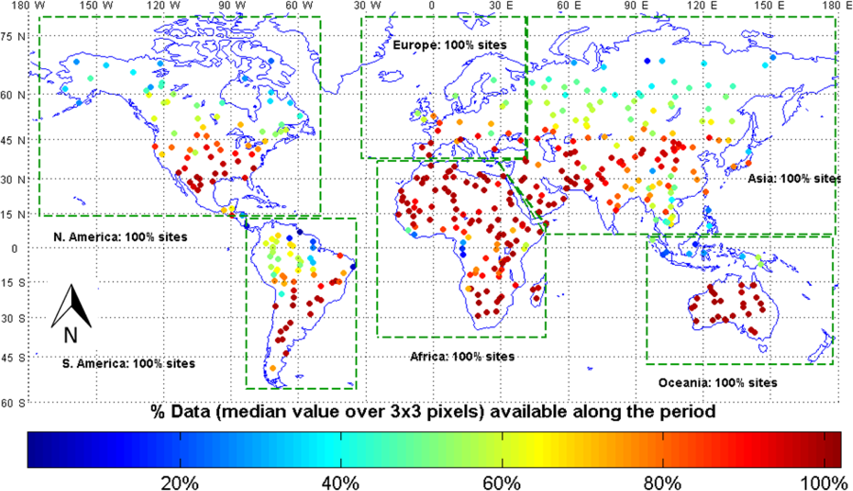
The validation exercise is performed over two ensembles of sites, BELMANIP2.1 (BEnchmark Land Multi-site Analysis and Intercomparison of products [41]) and DIRECT sites [18,20]. The 445 BELMANIP2.1 sites present the same distribution of vegetation types and conditions as the Earth’s surface while showing little topography and good level of homogeneity [41]. The land cover homogeneity of each site was double checked using the GLOBCOVER map [42,43], and the Google Earth engine. The 113 DIRECT sites include those where ground measurements of LAI and/or FAPAR and/or fCover are available from 2000. For most of these DIRECT sites, measurements were acquired only once during the growing season. The BELMANIP2.1 and DIRECT sites coordinates are available at [40] (Figure 1). Information such as literature references or web sites is also provided for DIRECT.
Running a validation exercise starts by selecting the products of interest. Although the number of products is not limited in the current implementation of the system, it is advised to validate at maximum 4 products for the sake of readability of the figures. For each product, several characteristics must be selected: the period (starting and ending years), product identification name in the figures and tables, and the Quality Assessment (QA) values considered for the validation. Finally, the output format of the figures (png, pdf, jpg) and the name of the validation exercise must be filled.
Once the characteristics of the products are selected, the validation exercise can be triggered. It consists in a suite of steps that are listed below and illustrated in section 4 for FAPAR products:
Description of the validation exercise: the products associated to the QA values considered as valid, the spatial domain and the selected period. Then, the corresponding fraction of data available per biome and continent is computed.
Analysis of the continuity of the products, mostly focusing on the fraction of missing data and their spatio-temporal distribution.
Computation of the temporal profiles of the products for a qualitative assessment of the main features of each product with regards to continuity, smoothness, magnitude and seasonality.
Evaluation of the temporal consistency with emphasis on the smoothness of the time series and the stability across years.
Comparison of the bulk distribution of the product values per biome type and per continent.
Comparison between products per biome type and continent using scatterplots and associated statistics.
Comparison with ground-based measurements (direct validation) for the quantification of product accuracy.
2.3. Importing New Data to Build a Reference and Benchmarking Data Base
Two types of data can be imported and hosted by OLIVE: new satellite land products to be validated and new ground-based measurements used for accuracy assessment (direct comparison).
Import new product: This facility allows producers to evaluate the performances of a new product as compared to existing ones in the system. Three files must be uploaded: (i) a metadata file which describes the product based on the GECA standard (Generic Environment for Cal/Val Analysis [44]; (ii) a description of the sites and dates covered by the product that must correspond to a significant subset of BELMANIP2.1 sites (at least over one continent), and (iii) the product value over the sites and dates described previously. The extracts must follow a specific format described in the OLIVE information page. Once these files are prepared, the user can upload them to the OLIVE platform. The new data can be published to make it accessible to the whole community or not. The new product is then listed along with the other available products.
Add new ground-based measurements: they can be added to expand the database of already available ones. This requires uploading the site description, methods used to complete and process the ground measurements, the strategy used to upscale the local ground measurement to the whole area covered by the site and the data themselves. The site should be at least 3 × 3 km2 in order to account for the geo-location uncertainties and the point spread function of the products [24]. Then, the CEOS-LPV sub-group will check if the proposed site complies with the CEOS recommendations for product validation before formally accepting it.
2.4. Sustainability of Validation
The OLIVE system facilitates improvement of the validation process through updating some functionality, enhancing the metrics used as well as the format of the outputs. The maintenance and update of the OLIVE system is overseen by the CEOS-LPV sub-group. Further, Essential Climate Variables (ECV) other than LAI, FAPAR and fCover such as surface albedo could be included in the OLIVE system for consistent validation. The OLIVE system is built in such a way that the code used to process the data can be modified by the CEOS_LPV sub-group. It is written in ®Matlab. The code is compiled and then run as an executable within the OLIVE web platform. As soon as the input and output file formats managed by the interface remain the same, the Matlab® (Mathworks, Natick, MA, USA) validation core code can be modified and updated.
3. Illustration of OLIVE Functionalities Based on FAPAR ECV
This section illustrates the main functionalities of the OLIVE platform applied to three available FAPAR products. After presenting the corresponding FAPAR definitions that can be found on the OLIVE platform, we describe and provide the results of the OLIVE validation exercise.
3.1. FAPAR Definition
FAPAR is recognized as an ECV [45]. Solar radiation in the spectral range 400 to 700 nm, known as Photosynthetically Active Radiation (PAR), provides the energy required by terrestrial vegetation to grow [1]. The part of this PAR that is effectively absorbed by plants is called the Fraction of Absorbed Photosynthetically Active Radiation (FAPAR). It is a non-dimensional quantity varying from 0 (over bare soil) to almost 1 for the largest amount of green vegetation. Since FAPAR is mainly used as a descriptor of photosynthesis and evapotranspiration processes, only the green photosynthetic elements (leaves, needles, or other green elements) should be accounted for. FAPAR also depends on the illumination conditions, i.e., the angular position of the sun and the relative contributions of the direct and diffuse incoming radiation. Both black-sky (assuming only direct radiation) and white sky (assuming that all the incoming radiation is in the form of isotropic diffuse radiation) FAPAR values may be considered [46]. The definition of the three products considered in this study is the black-sky FAPAR for a sun position at the satellite overpass.
3.2. Description of the Three FAPAR Products
3.2.1. GEOLAND Version1 (GEOV1)
GEOV1 [47] is derived from SPOT/VEGETATION sensors with a 10-day temporal sampling and 1/112° (about 1km at equator) ground sampling distance, in a Plate Carrée projection for the period 1998 (December) up to present [48].
Algorithm inputs are the same as for CYCLOPES [3], i.e., atmospherically corrected red, near-infrared and shortwave-infrared reflectances; normalized to a standard view-illumination geometry (nadir viewing, sun zenith angle corresponding to the median value in the compositing period) and with automatic outlier rejection [49]. The directional normalization is achieved by a parametric model inversion over data acquired during a 30 days compositing window period shifted every 10 days [50]. GEOLAND version 1 products are estimated using a neural network trained on values issued from the fusion of CYCLOPES [3] and MODIS Collection 5 products [6] to take advantage of their specific performances while limiting the situations where they show deficiencies. The learning data base was composed of the BELMANIP2.1 extracts of CYCLOPES L3A normalized reflectance products and the weighted sum of corresponding CYCLOPES and MODIS FAPAR products. FAPAR products correspond to the black sky values at 10:00 solar time.
A quality assessment flag value indicates when the retrieval algorithm fails (QA = 1), i.e., when there are less than two cloud- and snow-free observations in the compositing period (30 days) or when the retrieval is out of the valid range.
3.2.2. JRC-FAPAR (MGVI0)
MGVI (MERIS Global Vegetation Index) is a FAPAR product derived from MERIS sensor with a 10-day temporal sampling for the period (June) 2002 up to (April) 2012 [10,51]. Algorithm inputs are the daily L1b MERIS top of atmosphere (TOA) reflectances in the blue (band 2), red (band 8), near-infrared (band 14). MGVI is computed from the formulae provided in [10]. The 10 days synthesis is performed according to [52] and consists in selecting the MGVI value that is the closest to the average valid value over the 10 day synthesis. Valid values are identified using the MERIS L1b flag. FAPAR products correspond to the instantaneous black sky value at the time of satellite observations (about 10:30 solar time).For practical considerations, MERIS L1b TOA reflectances for BELMANIP2.1 and DIRECT sites were extracted and projected in the UTM (WGS84) at 1 km resolution while the MGVI computation and synthesis was performed by EMMAH, INRA. Note that the results obtained were checked with JRC to be compliant with the official MERIS MGVI instantaneous product value. However, we were not able to check the compositing algorithm because of the unavailability of time series extracts over BELMANIP2.1 or DIRECT sites. For this reason, this FAPAR product will be named as MGVIo in the following of the study as they do not correspond to the official product. We also associate a quality assessment flag (QA) value indicated when the retrieval algorithm fails, i.e., when no valid value is available within the 10 day synthesis. Therefore, for MGVI, QA = 0 indicates that the data was valid and QA = 1 indicates that the data was not produced.
3.2.3. Terra MODIS FPAR Collection 5 Product (MODC5)
MODC5 products [6] are available at WWW4. Collection 5 was produced between February 2000 through present at an 8-day time step and 1km resolution over an integrized sinusoidal grid.
MODIS main algorithm is based on a three-dimensional radiative transfer canopy model inversion based on Look Up Tables (LUT) [53,54]. Red and near-infrared atmospherically corrected MODIS reflectance [55,56] and the corresponding illumination-view geometry are used as inputs. The output is the mean FAPAR (and LAI) values averaged over the set of acceptable solutions for which simulated MODIS surface reflectances agree within specified level of model and measurement uncertainties. When the main algorithm fails, a backup algorithm based on NDVI (Normalized Difference Vegetation Index) relationships, calibrated over the same radiative transfer model simulations is used. MODIS FAPAR retrieval is executed irrespective of cloud and snow state but the majority of retrievals under these conditions or with residual atmospheric contamination are performed with the back-up algorithm [57,58].
The main and backup algorithms are defined for 6 biome types as considered by the MODIS land cover map product [59,60]. MODIS algorithm accounts for vegetation clumping at the canopy and leaf (shoot) scales through 3D radiative transfer formulations. The clumping at the landscape scale is partly addressed via mechanisms based on radiative transfer theory of canopy spectral invariants [53,61,62].
MODISC5 FAPAR product corresponds to the instantaneous value at the time of the satellite overpass. FAPAR values are first produced daily. Then, the 8 days composite corresponds to the values of the product when the maximum FAPAR value within the eight day period is observed. Note that FAPAR values are not retrieved over bare and very sparsely vegetated area, permanent ice and snow area, permanent wetland, urban and water bodies.
TERRA MODIS Collection 5 BELMANIP2.1 and DIRECT site extraction was performed at EMMAH, INRA. As the original MODIS projection is sinusoidal, the products were re-projected and extracted in Plate carrée (1/112° resolution) using the MODIS reprojection tool [63]. A value of FAPAR = 0 was set over pixels identified as bare and very sparsely vegetated area. Note that the initial TERRA MODIS quality flags were recombined to associate QA to the OLIVE extracts: QA = 0 indicates that the data were retrieved using the main algorithm without saturation, QA = 1 that they were retrieved using the main algorithm with saturation, QA = 2 using the back-up algorithm while a QA = 3 indicates that no product was retrieved.
3.3. The Validation Exercise
To avoid a large number of figures, we illustrate the main results derived from an OLIVE validation exercise. The complete report can be downloaded from [40] in html format.
3.3.1. Spatio-Temporal Domain Used for the Validation
The temporal domain used for the validation is defined by the starting and ending year for each product along with the QA threshold selected for considering a product as valid (Table 2). A pixel at a given date is considered valid if its QA value is below the QA threshold value given in Table 2.
The spatio-temporal sampling over the BELMANIP2.1 and DIRECT sites was adapted to each evaluation criteria to optimize statistics computation (Table 3): for those involving independent evaluation of the products (continuity, temporal consistency and stability, distributions), OLIVE uses the individual valid pixels extracted over a 49 × 49 pixels window centered over each BELMANIP2.1 site with their original temporal sampling (Table 2). This extent of 49 × 49 pixels was chosen to keep a good compromise between the size of the area that should be large enough to be the most representative, the homogeneity of the sites, and the corresponding data volume to be uploaded on the OLIVE platform. For the qualitative assessment of the temporal profiles of each site, the median value of the valid pixels over the central 3 × 3 pixels window is computed if at least 5 out of the 9 pixels are valid. If less than 5 pixels are valid, the data are declared invalid for the given date. The 3 × 3 pixel sampling is used to account for the geo-location uncertainties and the point spread function associated to the projected products making the spatial support more consistent across the investigated products [24].
For the pairwise comparison of products where both the spatial and temporal supports must be consistent, the median of the 3 × 3 valid pixels is first computed, as for the temporal profiles. Then, a monthly value centered on the 15th of the month is calculated using a weighted average of valid median values. The weighting function takes into account the temporal frequency and temporal resolution (Rt) of each product: the weight attributed to each day d corresponding to a valid product within a month is proportional to the number of days within the t ± Rt day period that belongs to the month.
Finally, for accuracy assessment based on the DIRECT sites, the median over the 3 × 3 valid pixels is first computed. Then, OLIVE provides two methods to make ground-based measurements and satellite product dates concomitant. First, the valid product that is the closest to the date of ground measurement acquisition (within a ±15 day period) is selected. This allows comparison with product values as similar as possible to the original ones. Second, the product is interpolated at the measurement date using the LOWESS algorithm [64] for a 2 month window span. This last process allows smoothing of the high frequency variability of the product while exploiting ground measurements that are not exactly located at the date of the product availability.
For both pairwise comparison of products and accuracy assessment, we compute the slope and intercept of the linear regression between the y and x axis. We also compute the associated root mean square error (RMSE) and the coefficient of determination (R2), and specify the number of data (N) that were used to calculate these quantities.
3.3.2. Continuity Assessment
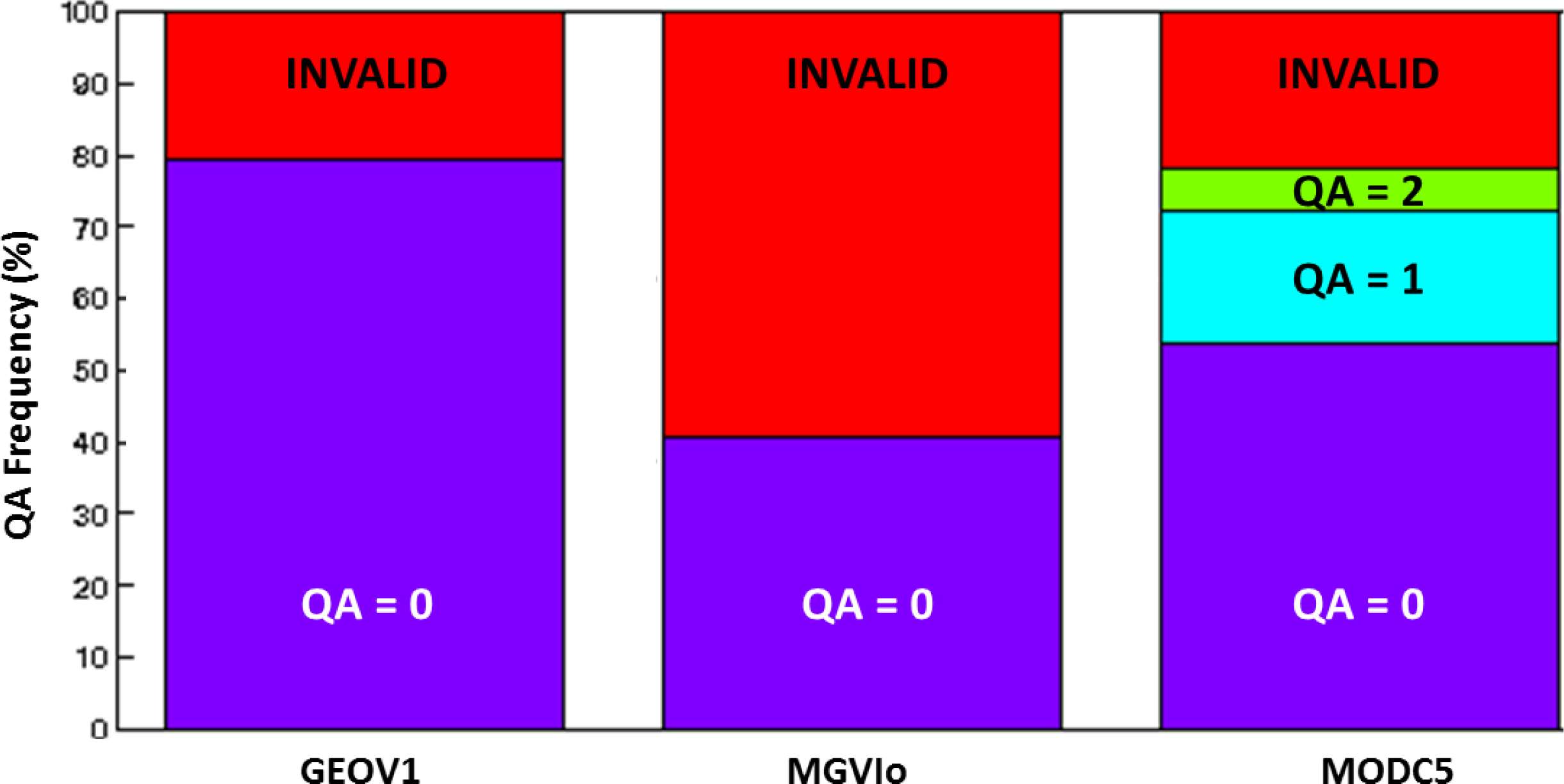
Continuity is assessed as the fractions of valid (and non-valid) data as well as their distribution in space and time. It is computed over 49 × 49 valid pixels of the BELMANIP2.1 sites with the original temporal sampling (Table 2). The fraction of valid data for the considered period is provided at several levels including: global level, site level and continental level (results not reported here for the sake of brevity but available in the validation report). In addition to providing information on the continuity of the products, it also allows evaluating the degree of completion and reliability of the validation exercise.
The global distribution is detailed per QA level (Figure 2) and shows that GEOV1 and MODC5 provide product values in most situations, whereas MGVIo shows a large fraction of invalid data. Note that the back-up algorithm (QA = 2) for MODIS is used in about 5% of the cases, whereas the main algorithm is under saturation situations (QA = 1) in about 20% cases.
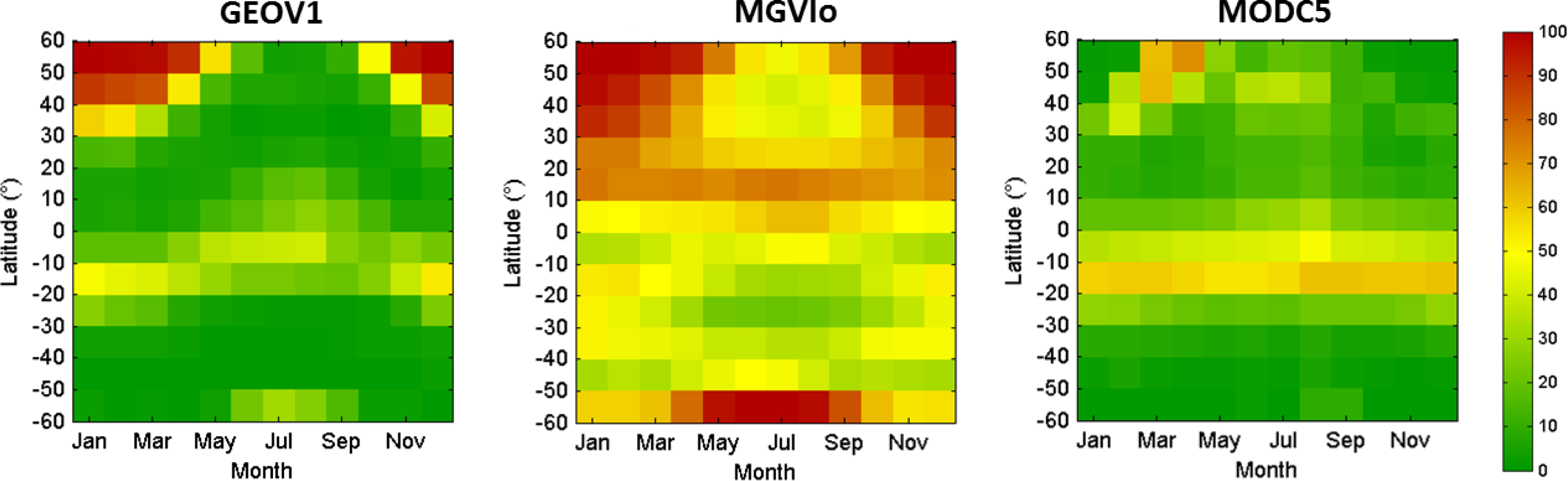
The spatio-temporal distribution of the fraction of invalid data is computed for each product at the monthly time step and per 10° latitude strips (Figure 3). As expected, it decreases around the equator because of large occurrence of clouds, as well as for the higher latitudes for GEOV1 and MGVIo due to short day length and poor illumination conditions in addition to the cloud occurrence. This is not observed for MODIS because of the exploitation of the replication of views for the higher latitudes that are fully exploited, in agreement with the results reported by [65].
The fraction of valid data is also evaluated per continent and site (Figure 4) and per biome type. The GLOBCOVER biome classification is used [42,43] with the classes being aggregated into larger biome types comprising of Evergreen Broadleaf Forest (EBF), Evergreen Needleleaf Forests (ENF), Deciduous Broadleaf Forest (DBF) and Non Forest (NF). GLOBCOVER was chosen in order to be consistent with the BELMANIP2 site selection and homogeneity verification. However, considering the broad categorization of the vegetation after aggregation, the impact of using a different land cover map should be marginal. The results on the distribution of the fraction of valid observations per biome type showed good consistency with the spatio-temporal distribution (Figure 3) and is detailed in the OLIVE validation report. It can be noted also that in recent years, smoothing and gap filling methods were developed to overcome the problem of missing data [16,66–68].
3.3.3. Temporal Profiles
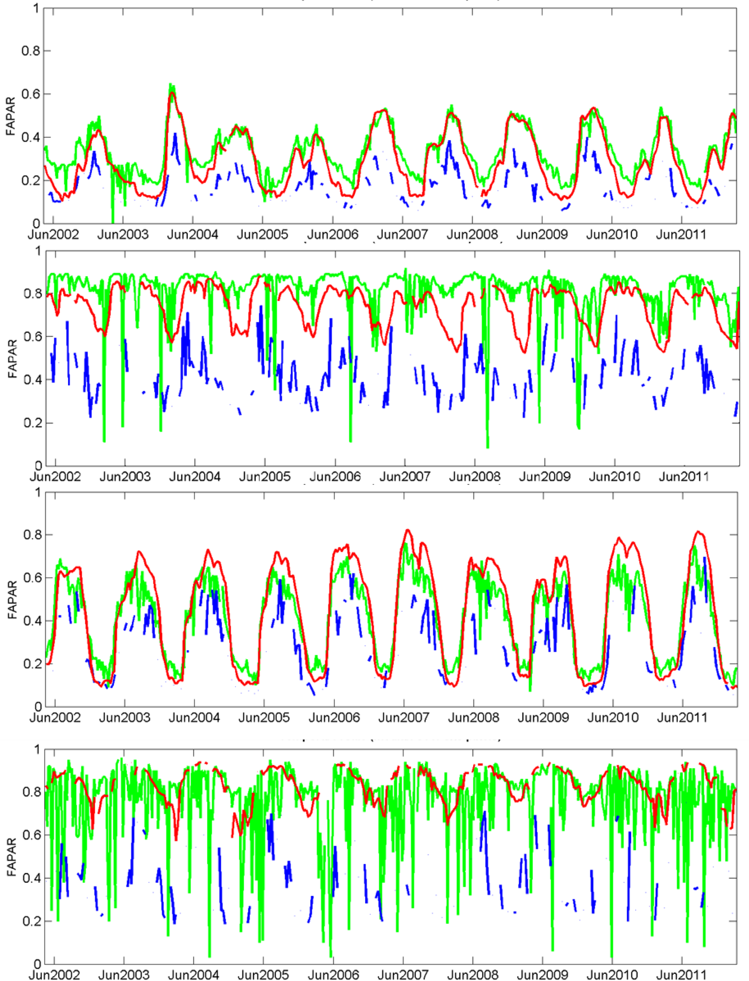
The temporal profiles are produced for each BELMANIP2.1 and DIRECT site. They allow identifying qualitatively the main features of each product. Figure 5 presents a selection of 4 sites corresponding to the four main biomes considered in OLIVE (BELMANIP2.1, Sites number 5, 65, 165 and 320), the other temporal profiles being available in the full OLIVE report (WWW1). The temporal profiles show a general agreement of the seasonality for the non-forest and deciduous broad leaf forest sites (Figure 5). For the needleleaf forest and evergreen broadleaf forest, we observe some discrepancies, particularly for MGVIo, which shows more missing observations confirming the previous results on continuity assessment. MODIS and MGVIo show also high frequency variations associated to the shorter temporal resolution as compared to GEOV1. However, one of the main features observed is the difference in magnitude for MGVIo that shows almost systematically lower FAPAR values. This was already reported in previous studies [23,36–39] and could be explained mainly by differences in algorithm design where different assumptions on canopy structure and leaf optical properties are used.
3.3.4. Temporal Consistency: Smoothness and Stability
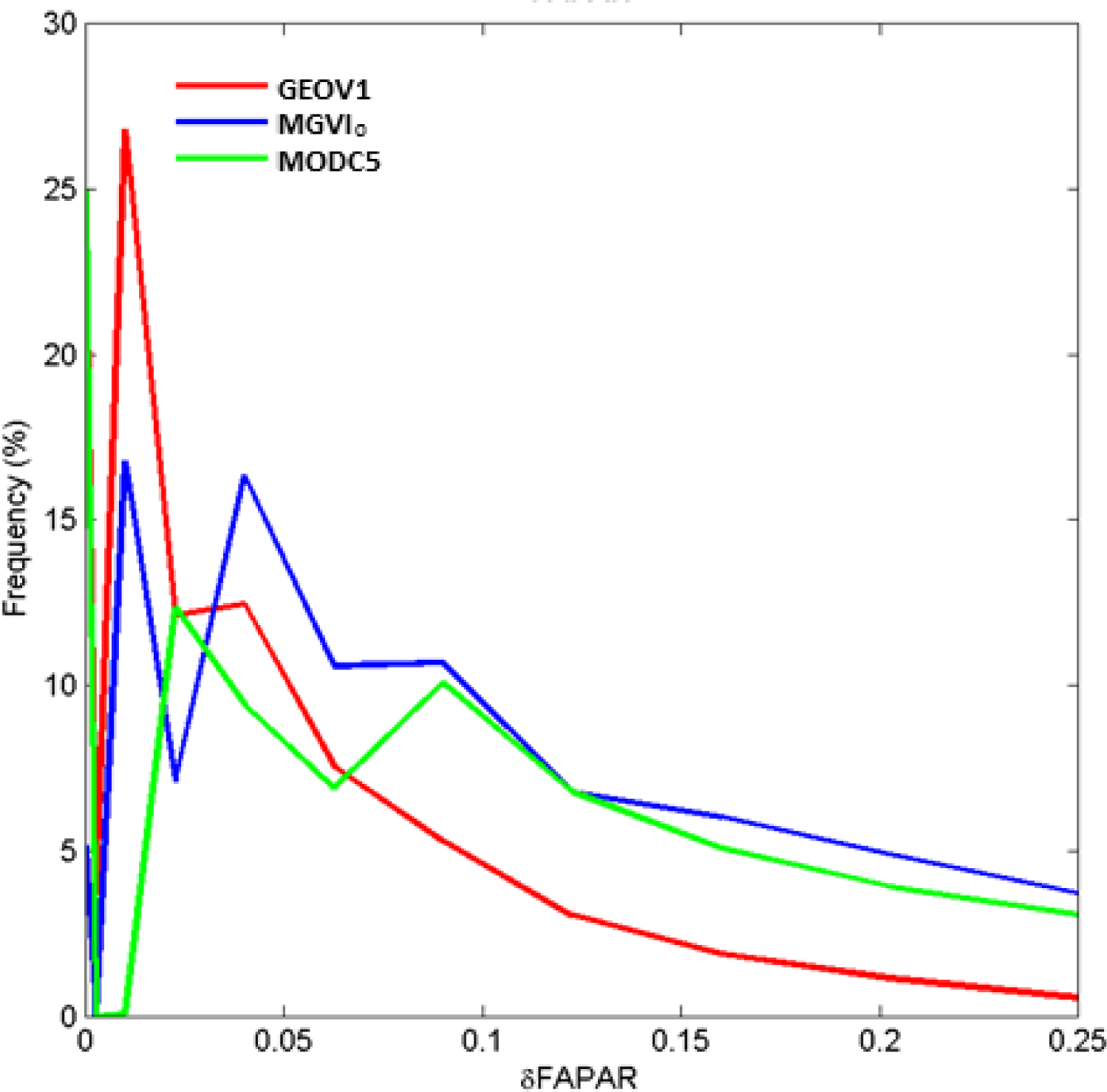
Considering the product temporal frequency, the temporal course of FAPAR and hence the products are expected to be smooth because the corresponding biophysical variable changes incrementally except in the case of disturbance. Smoothness was characterized by using the absolute difference δ between the product value at date t, P(t), and the mean value between the two bracketing dates δ = |1/2(P(t + Δt) + P(t)) − P(t)|, where Δt is the temporal sampling interval [24]. The difference δ is computed only if the two bracketing product values (P(t− Δt) and P(t + Δt)) exist. The smoother the temporal evolution, the smaller the δ difference should be. The smoothness δ is computed separately for each product for all the acquisition dates over the whole period considered (Table 3), and the 49 × 49 pixels centered on the BELMANIP2.1 sites using the original temporal sampling (Table 2). The results show that GEOV1 is generally smoother than MODIS and MGVIo, confirming the qualitative observations over the temporal profiles (Figure 6). This is mainly due to the longer temporal compositing window (30 days).
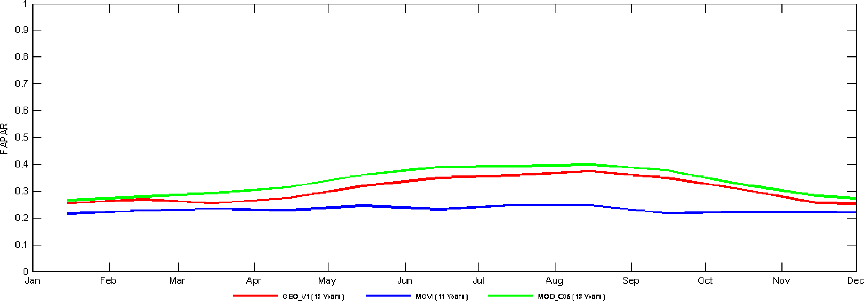
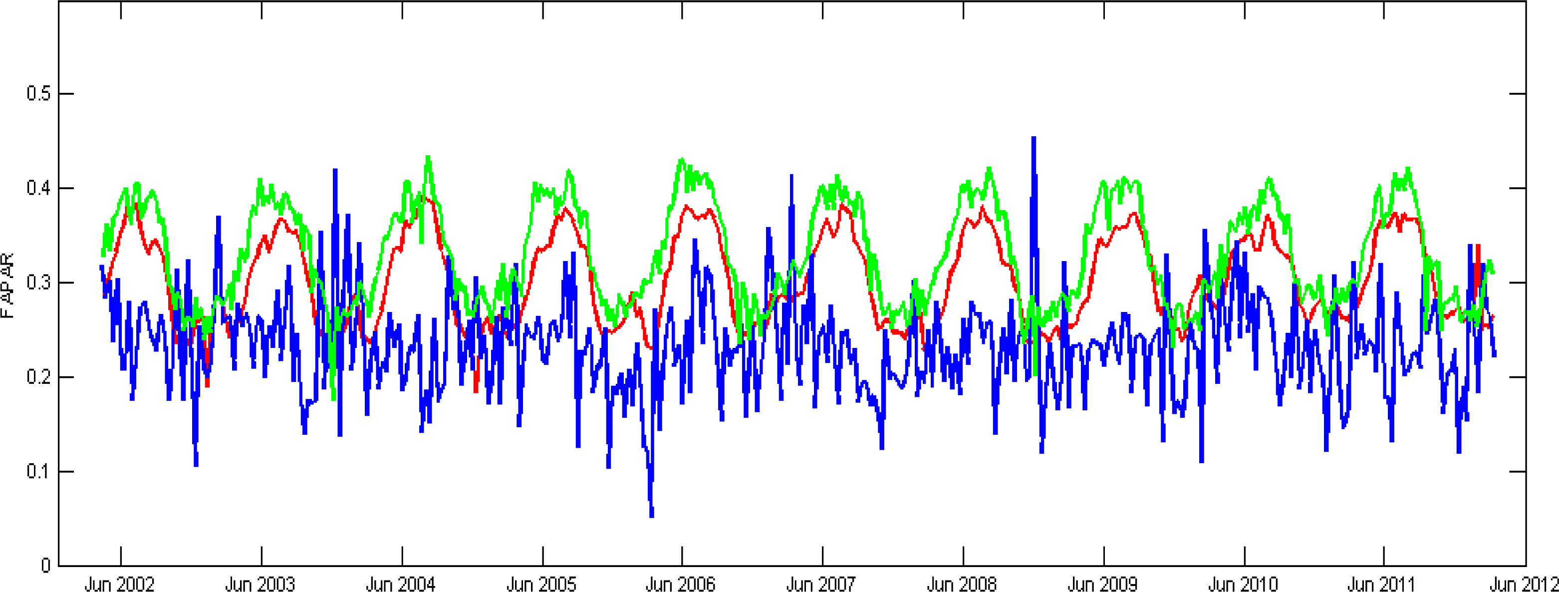
To better assess the temporal stability of the products, a global average is computed for each date over the 49 × 49 pixels of all the BELMANIP2.1 sites. The results (Figure 7) confirm the fair agreement between MODIS and GEOV1 FAPAR products with consistent year to year seasonality. Conversely, MGVIo shows both high and low frequency variability, for example, in June 2004, 2008 and 2009 MGVIo displays an anomaly in FAPAR seasonality that is not observed with MODC5 and GEOV1. A yearly climatology is finally computed to provide a global average seasonality (Figure 8). The difference in magnitude is the largest in July, corresponding to the maximum FAPAR value, with MODC5 > GEOV1 > MGVIo. Conversely, the spatial and inter-annual averages of the three products are in relatively good agreement in winter. Note however that the spatial representativeness may differ between the three products, depending on the fraction of valid data (Figures 2 and 3).
3.3.5. Distribution Per Biome and Continent
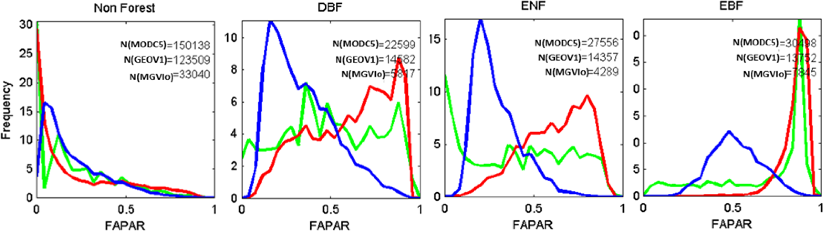
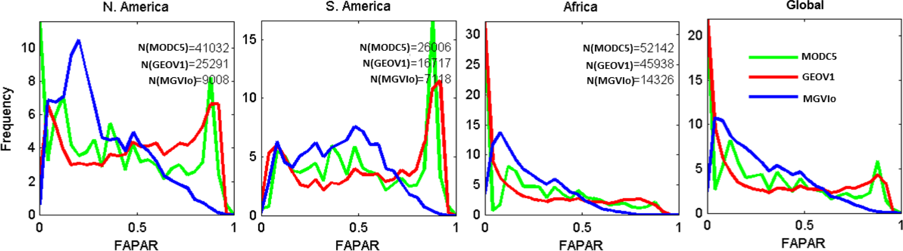
The histograms (probability density function) of each product were computed for the 4 main biome types (NF, DBF, ENF and EBF) over the valid pixels within the 49 × 49 pixel window centered over all the BELMANIP2.1 sites for the valid dates and for the considered period (Table 3) using the original temporal sampling (Table 2). Results show that MODC5 and GEOV1 have similar distributions while some differences are observed for Evergreen Needleleaf Forests (Figure 9). MODC5 shows an unexpected large number of almost bare soil situations. This is probably due to a misclassification of pixels into bare area, for which the MODIS algorithm is not triggered, and that were set to null FAPAR value in OLIVE. Conversely, GEOV1 shows a pronounced mode for high values of FAPAR. MGVIo modes are systematically shifted towards the low FAPAR values except for the Non Forest sites (Figure 9). Further, maximum FAPAR values for the forest biomes hardly reach FAPAR = 0.8 although such biomes, which have an almost complete cover fraction in many situations, should show higher values of FAPAR. In addition, the significant fraction of almost bare soil situations seen in GEOV1 and MODC5 for the Non Forest sites (Figure 9) is not seen by MGVIo.
The observed distribution over continents (only three are displayed here) and for the global distribution (Figure 10) show similar features as those observed over the main biome types: relatively good agreement between MODC5 and GEOV1, while MGVIo shows higher fraction of low FAPAR values including very low values.
3.3.6. Pairwise Comparison between the Three Products
The same spatial and temporal support is used to provide scatterplots between products: the median over the valid 3 × 3 pixels centered over each site is computed and then interpolated for fixed dates every 15th of the month during the considered period (Table 2). Scatterplots were generated globally for each pair of products (all BELMANIP2.1 sites, Figure 11) and as a function of the main biome types (results not presented).
Results show that MODC5 and GEOV1 are fairly consistent over the whole range of FAPAR values. However, an offset around 0.1 is observed for MODC5 for the very low GEOV1 FAPAR values as already noticed by [18]. The dissymmetry in the scattered points under the 1:1 line is mainly explained by the high frequency variability observed in MODC5, partly due to cloud contamination that negatively impacts the estimated FAPAR value (Figure 11). MGVIo shows consistent values with GEOV1 for the lowest FAPAR values while MODC5 is offset by 0.1 in the same conditions, in agreement with the offset value already observed with GEOV1. For the medium to high FAPAR values, MGVIo shows systematically lower values, compared to GEOV1 and MODC5, with the differences increasing with FAPAR values and reaching up to 0.3 for the highest FAPAR values.
3.3.7. Accuracy Assessment Using Actual Ground Measurements
Most of the DIRECT sites were sampled using Digital Hemispherical Photographs (DHPs) and processed using can-eye (WWW6) for 10:00 local solar time. DHP provides FIPAR (Fraction of Intercepted Photosynthetically Active Radiation) rather than FAPAR, but the difference between both is marginal, except for highly homogeneous canopies [11,45,46]. Therefore the consistency between satellite products and ground validation measurements is ensured at the exception of non-green elements. Indeed for the forest sites the impact is expected to be small since they have mainly been sampled during the peak of the growing season, the leaves at the top of the crown masking the trunks and branches. For the other sites, cases with large amount of non-green vegetation were discarded.
The comparison with ground-based measurements was performed using the two methods proposed in Table 3 that is either using the product value period the closest to the ground measurement date (±15 days) or the value interpolated at the date of the ground measurement. It should be noted that evergreen needle leaf or broadleaf forest sites were treated as special cases to accommodate situations when the ground campaign is outside the validation exercise period (Table 2). This allows exploiting additional ground measurements: for each year of the validation exercise time period, the median of the product values is computed at the date in the year at which the measurement acquisition was achieved. Indeed, these specific sites are expected to show some limited inter-annual stability, and can be checked against the temporal profiles available for all the DIRECT sites. They are identified as open symbols in the results (Figure 12).
Results show that the use of the closest observation reduces the number of available matches between ground measurements and available products (Table 4). This is mostly obvious for MGVIo where only 18 DIRECT sites could be used because of the larger fraction of missing data as compared to 60 when the products values were interpolated with time. For MODC5 and GEOV1, the performances measured with the “closest” product are very similar to those obtained with the “interpolated” product values (Table 4), except that the RMSE of MODC5 is much higher with the “closest” method. This is explained by the high frequency variability observed on MODC5 temporal profiles that is partly smoothed out using the interpolation method. Emphasis here is therefore on the performances as measured by the “interpolated” method since it allows more data points as well as smoothing out the high temporal variability that is not necessarily targeted when addressing accuracy assessment. The high temporal variability is one of the main components of the precision of the products. Note that the 3 × 3 spatial support already smoothed out the random variability associated to the products at the pixel level.
Detailed inspection of the results obtained with the method based on temporal interpolation shows that GEOV1 achieves the best performances with a RMSE value of 0.12 (Table 4) followed closely by MODC5 (RMSE = 0.14). MODC5 shows an intercept of 0.18 for the low FAPAR values (Figure 12), confirming the previous observations derived from the inter-comparison exercise (Figure 11). The comparison with ground measurements confirms MGVIo underestimation as already observed by [33] and [69], particularly for the high FAPAR values.
The RMSE values obtained in this study appear to be slightly above the targeted uncertainties values required within the Global Climate Observing System GCOS [1], i.e., the value of 0.05% or 10% for FAPAR. However the uncertainties associated to the ground measurements also need to be accounted for. Regarding the number of data points that are considered (Table 4), and given their distribution in the [0, 1] possible range over several vegetation types, the validation stage 2 is achieved, making significant progress toward stage 3 validation.
4. Discussion
OLIVE provides metrics to evaluate the continuity of the products (missing data, length of gaps). It showed some deficiencies of the three FAPAR products considered in this study. They are mainly due to cloud occurrence over the low latitude areas and the limited day length in winter for the higher latitudes that make reflectance data unavailable. It should be noted that these differences, observed on the product continuity, may affect the evaluation of the uncertainties against ground measurements. Indeed, it slightly changes the representativeness of the ground data with regards to the global range.
The validation procedures should be improved by providing more details on the structure of the uncertainties which is one of the main outputs of the validation exercise expected by the user community. Uncertainties are derived from several components including precision (random variability), accuracy (bias, as referring to a systematic measurement error [70]) and stability (drifts of the accuracy with time). In OLIVE, the precision is approached looking at the high frequency variability at the pixel scale and using the original temporal sampling of the products (Figure 6). The accuracy is evaluated by comparison with upscaled ground measurements. Products are temporally (LOWESS filter [64] and spatially (median over 3 × 3 pixels) smoothed to provide spatial and temporal supports similar to that of the upscaled ground measurements. This processing of the original product minimizes the high frequency variability making the metrics more sensitive to bias. However, the accuracy assessment is limited by the number of available ground measurements that reduces the targeted global representativeness both spatially and temporally. Most of the DIRECT sites were only measured once within the entire data record period. However, it is critical to validate the seasonality in the temporal profiles. Furthermore, a significant percentage of DIRECT sites correspond to non-forest situations. Additional sites over forested areas with medium to high FAPAR values are required to improve the accuracy assessment. Further, situations including more complex topography that represent a significant part of the vegetated area should also be sampled. Therefore, the OLIVE tool allows the community to extend the ground validation data sets by adding ground measurement compatible with the medium sensor resolution, through an open, simple and fast submission process.
Finally, the accuracy assessed from the ground validation also integrates the uncertainties associated to their measurements, while the upscaling process smoothes out most of the random component of the uncertainties, biases may still be observed. FAPAR is derived from transmittance measurements and a significant fraction of non-green vegetation elements may be taken into account in some situations, inducing an overestimation of the actual FAPAR values. However, most of the situations where this artifact is expected to be significant are not considered in OLIVE (deciduous forests in winter time, grasslands and crops after the peak of growth). Finally, for the forest situations, the presence of a green understory has to be accounted for in the computation of the canopy FAPAR value. All situations where a significant green understory was not accounted for are excluded from OLIVE. This explains also why the number of forest cases available for accuracy assessment is limited.
The quantification of the stability is critical when evaluating trends due to the possible impacts of global change over several decades or when looking for anomalies. Specific metrics still need to be incorporated into OLIVE to evaluate the stability e.g. for the recently released long term series derived from AVHRR [16,71].
The validation of satellite products is a complex exercise that requires assessment across several spatial (pixel, site, region, continent, biome) and temporal scales (high frequency, seasonality and inter-annual trends). Methods were applied here to satellite derived FAPAR products, but may be extended to FAPAR simulated by dynamic global vegetation models to better evaluate their degree of agreement with remote sensing products as well as ground measurements. The OLIVE system is a software implementation that addresses GCOS and subsequently CEOS-LPV recommendations for obtaining consistent and reliable validation results. However, the metrics addressed should evolve to define a more detailed picture of the uncertainties associated to the satellite derived products. The OLIVE system has been designed to allow updating the validation code as well as implement improvements endorsed by CEOS-LPV. More efforts should be dedicated to a better knowledge of the uncertainties associated to the products in their original format. The decomposition into precision, accuracy and stability is a first step, but each of these components has a proper structure that should ideally be retrieved from the validation exercise. This will mainly need additional ground measurement sites and a better knowledge of the associated uncertainties. The validation activities of moderate resolution (250 m for MODIS and VIIRS, 300 m for MERIS, PROBA-V and Sentinel 3) will ease the validation process by allowing more sites with already available ground measurements. Flux tower networks are expected to widely contribute to the validation of hectometric and decametric spatial resolution products. Further, recent technical developments in measurement devices [72] allow to spatially distribute ground instruments, and perform a FAPAR temporal monitoring throughout time based on PAR radiation measurements.
5. Conclusions
The OLIVE platform is available on the ESA CAL/VAL portal [40]. It provides key information to the user community regarding a synthetic description of the variables of interest and the corresponding satellite derived estimates. OLIVE should therefore bring benefit to the community allowing benchmarking, improvement and an independent objective validation of existing and future products. The current status of the validation exercise shows that stage “2.5” (between 2 and 3) is reached for FAPAR with accuracy performances that still do not completely fulfill GCOS requirements [1]. With the contribution of the scientific community to provide suitable ground experiments to the platform, OLIVE offers a way to reach stage 3 (validation against ground measurements over multiple locations and time periods to represent the global range) and 4 with regular updates of the validation results, including the addition of new LAI, FAPAR and FCOVER products by the developer community.
OLIVE has the potential to be extended to other biophysical products including land surface albedo and soil moisture with very minor adaptations. Discrete variables, such as land cover and burnt areas, will require substantial modifications as their validation requires specific procedures and metrics. The validation of biophysical products with higher spatial resolution, as for example provided by LANDSAT-8 and the upcoming Sentinel-2 (10 m–60 m) missions, should capitalize on the OLIVE platform, although requiring significant changes in the validation reference data and procedures.
Acknowledgments
The OLIVE project was funded by the European Space Agency and supported by the CEOS-LPV subgroup. The authors would also like to thank the many individuals who contributed to the different projects (BigFoot, VALERI, CCRS activities, MODLAND activities…) that allowed gathering all the ground measurements available in the OLIVE platform since they represent a huge effort and manpower investment.
Author Contributions
Marie Weiss and Frédéric Baret are the principal authors of this manuscript having written the majority of the manuscript and contributing at all phases of the investigation. Tom Block, Bettina Scholze and Carsten Brockmann have implemented the OLIVE web service on the CEOS CAL/VAL portal maintained by Alessandro Burini. They have also extracted the BELMANIP2 and DIRECT sites for MERIS data, while Nadine Gobron checked the MGVI computation from these data. Benjamin Koetz is the ESA project officer who followed the OLIVE project. Ranga Myneni provided easy access to MODIS FPAR extracts. His participation was made possible through funding from NASA Earth Science Division. In addition, Joanne Nightingale, Gabriela Schaepman-Strub, Richard Fernandes, Stephen Plummer, Nadine Gobron, Arturo Sanchez-Azofeifa, Fernando Camacho, Ranga Myneni, as members of the CEOS LPV group; have reviewed this manuscript and provided comments and suggestions.
Conflicts of Interest
The authors declare no conflict of interest.
References
- Global Climate Observing System (GCOS). Global Climate Observing System—Systematic Observation Requirements for Satellite-Based Products for Climate-2011 Update, Supplemental Details to the Satellite Based Component of the Implementation Plan for the Global Observing System for Climate in Support of the UNFCCC (2010 Update). In GCOS-154; World Meteorological Organization: Geneva, Switzerland, 2011; p. 138. [Google Scholar]
- Veroustraete, F.; Patyn, J.; Myneni, R.B. Estimating net ecosystem exchange of carbon using the normalized difference vegetation index and an ecosystem model. Remote Sens. Environ 1996, 58, 115–130. [Google Scholar]
- Baret, F.; Hagolle, O.; Geiger, B.; Bicheron, P.; Miras, B.; Huc, M.; Berthelot, B.; Nino, F.; Weiss, M.; Samain, O.; et al. LAI, fAPAR and fCover CYCLOPES global products derived from VEGETATION: Part 1: Principles of the algorithm. Remote Sens. Environ 2007, 110, 275–286. [Google Scholar]
- Pisek, J.; Chen, J.M. Comparison and validation of MODIS and VEGETATION global LAI products over four BigFoot sites in North America. Remote Sens. Environ 2007, 109, 81–94. [Google Scholar]
- Plummer, S.; Arino, O.; Simon, W.; Steffen, W. Establishing an Earth observation product service for the terrestrial carbon community: The GLOBCARBON initiative. Mitig. Adapt. Strat. Glob. Chang 2006, 11, 97–111. [Google Scholar]
- Myneni, R.B.; Hoffman, S.; Knyazikhin, Y.; Privette, J.L.; Glassy, J.; Tian, Y.; Wang, Y.; Song, X.; Zhang, Y.; Smith, G.R.; et al. Global products of vegetation leaf area and absorbed PAR from year one of MODIS data. Remote Sens. Environ 2002, 83, 214–231. [Google Scholar]
- Xiao, Z.; Liang, S.; Wang, J.; Chen, P.; Yin, X.; Zhang, L.; Song, J. Use of general regression neural networks for generating the GLASS leaf area index product from time-series MODIS surface reflectance. IEEE Trans. Geosci. Remote Sens 2014, 52, 209–223. [Google Scholar]
- Pinty, B.; Andredakis, I.; Clerici, M.; Kaminski, T.; Taberner, M.; Verstraete, M.M.; Gobron, N.; Plummer, S.; Widlowski, J.L. Exploiting the MODIS albedos with the two-stream inversion package (JRC-TIP): 1. Effective leaf area index, vegetation, and soil properties. J. Geophys. Res: Atmos 2011, 116, D09105. [Google Scholar] [CrossRef]
- Bacour, C.; Baret, F.; Béal, D.; Weiss, M.; Pavageau, K. Neural network estimation of LAI, fAPAR, fCover and LAIxCab, from top of canopy MERIS reflectance data: Principles and validation. Remote Sens. Environ 2006, 105, 313–325. [Google Scholar]
- Gobron, N. ENVISAT’s Medium Resolution Imaging Spectrometer (MERIS) Algorithm Theoretical Basis Document: FAPAR and Rectified Channels over Terrestrial Surfaces; Joint Research Center: Ispra, Italy, 2011; p. 27. [Google Scholar]
- Gobron, N.; Pinty, B.; Taberner, M.; Mélin, F.; Verstraete, M.; Widlowski, J.L. Monitoring the photosynthetic activity of vegetation from remote sensing data. Adv. Space Res 2006, 38, 2196–2202. [Google Scholar]
- Chen, J.M.; Menges, C.H.; Leblanc, S.G. Global mapping of foliage clumping index using multi-angular satellite data. Remote Sens. Environ 2005, 97, 447–457. [Google Scholar]
- Roujean, J.-L.; Lacaze, R. Global mapping of vegetation parameters from POLDER multiangular measurements for studies of surface-atmosphere interactions: A pragmatic method and validtion. J. Geophys. Res 2002, 107, ACL6:1–ACL6:14. [Google Scholar]
- Verger, A.; Camacho, F.; García-Haro, F.J.; Meliá, J. Prototyping of Land-SAF leaf area index algorithm with VEGETATION and MODIS data over Europe. Remote Sens. Environ 2009, 113, 2285–2297. [Google Scholar]
- Ganguly, S.; Samanta, A.; Schull, M.A.; Shabanov, N.V.; Milesi, C.; Nemani, R.R.; Knyazikhin, Y.; Myneni, R.B. Generating vegetation leaf area index earth system data record from multiple sensors. Part 1: Theory. Remote Sens. Environ 2008, 112, 4333–4343. [Google Scholar]
- Verger, A.; Baret, F.; Weiss, M.; Lacaze, R.; Makhmara, H.; Vermote, E. In Long Term Consistent Global GEOV1 AVHRR Biophysical Products. Proceedings of 1st EARSeL Workshop on Temporal Analysis of Satellite Images, Mykonos, Greece, 23–25 May 2012; pp. 28–33.
- Weiss, M.; Baret, F.; Eerens, H.; Swinnen, E. FAPAR over Europe for the Past 29 Years: A Temporally Consistent Product Derived from AVHRR and VEGETATION Sensors. Proceedings of the Recent Advances in Quantitative Remote Sensing (RAQRS III), Valencia, Spain, 27 September–1 October 2010; Sobrino, J.A., Ed.; Publicacions de la Universitat de València: Valencia, Spain, 2010; pp. 428–433. [Google Scholar]
- Camacho, F.; Cernicharo, J.; Lacaze, R.; Baret, F.; Weiss, M. GEOV1: LAI, FAPAR essential climate variables and FCOVER global time series capitalizing over existing products. Part 2: Validation and intercomparison with reference products. Remote Sens. Environ 2013, 137, 310–329. [Google Scholar]
- Fang, H.; Jiang, C.; Li, W.; Wei, S.; Baret, F.; Chen, J.M.; Garcia-Haro, J.; Liang, S.; Liu, R.; Myneni, R.B.; et al. Characterization and intercomparison of global moderate resolution leaf area index (LAI) products: Analysis of climatologies and theoretical uncertainties. J. Geophys. Res.: Biogeosci 2013, 118, 529–548. [Google Scholar]
- Garrigues, S.; Lacaze, R.; Baret, F.; Morisette, J.; Weiss, M.; Nickeson, J.; Fernandes, R.; Plummer, S.; Shabanov, N.V.; Myneni, R.; et al. Validation and intercomparison of global leaf area index products derived from remote sensing data. J. Geophys. Res 2008, 113, G02028. [Google Scholar] [CrossRef]
- Gessner, U.; Niklaus, M.; Kuenzer, C.; Dech, S. Intercomparison of leaf area index products for a gradient of sub-humid to arid environments in West Africa. Remote Sens 2013, 5, 1235–1257. [Google Scholar]
- Kappas, M.W.; Propastin, P.A. Review of available products of leaf area index and their suitability over the formerly Soviet Central Asia. J. Sens 2012. [Google Scholar] [CrossRef]
- McCallum, I.; Wagner, W.; Schmullius, C.; Shvidenko, A.; Obersteiner, M.; Fritz, S.; Nilsson, S. Comparison of four global FAPAR datasets over Northern Eurasia for the year 2000. Remote Sens. Environ 2010, 114, 941–949. [Google Scholar]
- Weiss, M.; Baret, F.; Garrigues, S.; Lacaze, R.; Bicheron, P. LAI, fAPAR and fCover CYCLOPES global products derived from VEGETATION. Part 2: Validation and comparison with MODIS Collection 4 products. Remote Sens. Environ 2007, 110, 317–331. [Google Scholar]
- CEOS Land Product Validation Web Site. Available online: http://lpvs.gsfc.nasa.gov/ (accessed on 2 May 2014).
- Justice, C.O.; Starr, D.; Wickland, D.; Privette, J.; Suttles, T. EOS land validation coordination: An update. Earth Observ 1998, 10, 55–60. [Google Scholar]
- Morisette, J.; Baret, F.; Privette, J.L.; Myneni, R.B.; Nickeson, J.; Garrigues, S.; Shabanov, N.; Weiss, M.; Fernandes, R.; Leblanc, S.; et al. Validation of global moderate resolution LAI Products: A framework proposed within the CEOS Land Product Validation subgroup. IEEE Trans. Geosci. Remote Sens 2006, 44, 1804–1817. [Google Scholar]
- Tian, Y.; Woodcock, C.E.; Wang, Y.; Privette, J.L.; Shabanov, N.V.; Zhou, L.; Zhang, Y.; Buermann, W.; Dong, J.; Veikkanen, B.; et al. Multiscale analysis and validation of the MODIS LAI product: I. Uncertainty assessment. Remote Sens. Environ 2002, 83, 414–430. [Google Scholar]
- Yang, W.; Shabanov, N.V.; Huang, D.; Wang, W.; Dickinson, R.E.; Nemani, R.R.; Knyazikhin, Y.; Myneni, R.B. Analysis of leaf area index products from combination of MODIS Terra and Aqua data. Remote Sens. Environ 2006, 104, 297–312. [Google Scholar]
- Baret, F.; Nightingale, J.; Garrigues, S.; Nickeson, J. Report on the CEOS Land Product Validation sub-group meeting Missoula, Montana, 15 June 2009. Earth Observ 2009, 21, 26–30. [Google Scholar]
- Nightingale, J.; Schaepman-Strub, G.; Nickeson, J.; leads, L.F.A. Assessing Satellite-Derived Land Product Quality for Earth System Science Applications: Overview of the CEOS LPV Sub-Group. Proceedings of the 34th International Symposium on Remote Sensing of Environment, Sydney, NSW, Australia, 10–15 April 2011.
- Fensholt, R.; Sandholt, I.; Rasmussen, M.S. Evaluation of MODIS LAI, fAPAR and the relation between fAPAR and NDVI in a semi-arid environment using in situ measurements. Remote Sens. Environ 2004, 91, 490–507. [Google Scholar]
- Gobron, N.; Pinty, B.; Aussedat, O.; Chen, J.M.; Cohen, W.B.; Fensholt, R.; Gond, V.; Huemmrich, K.F.; Lavergne, T.; Mélin, F.; et al. Evaluation of fraction of absorbed photosynthetically active radiation products for different canopy radiation transfer regimes: Methodology and results using Joint Research Center products derived from SeaWiFS against ground-based estimations. J. Geophys. Res 2006, 111. [Google Scholar] [CrossRef]
- Pinty, B.; Jung, M.; Kaminski, T.; Lavergne, T.; Mund, M.; Plummer, S.; Thomas, E.; Widlowski, J.L. Evaluation of the JRC-TIP 0.01° products over a mid-latitude deciduous forest site. Remote Sens. Environ 2011, 115, 3567–3581. [Google Scholar]
- Steinberg, D.C.; Goetz, S.J.; Hyer, E.J. Validation of MODIS FPAR products in boreal forests of Alaska. IEEE Trans. Geosci. Remote Sens 2006, 44, 1818–1828. [Google Scholar]
- D’Odorico, P.; Gonsamo, A.; Pinty, B.; Gobron, N.; Coops, N.; Mendez, E.; Schaepman, M.E. Intercomparison of fraction of absorbed photosynthetically active radiation products derived from satellite data over Europe. Remote Sen. Environ 2014, 142, 141–154. [Google Scholar]
- Meroni, M.; Atzberger, C.; Vancutsem, C.; Gobron, N.; Baret, F.; Lacaze, R.; Eerens, H.; Leo, O. Evaluation of agreement between space remote sensing SPOT-VEGETATION fAPAR time series. IEEE Trans. Geosci. Remote Sens 2013, 51, 1951–1962. [Google Scholar]
- Pickett-Heaps, C.A.; Canadell, J.G.; Briggs, P.R.; Gobron, N.; Haverd, V.; Paget, M.J.; Pinty, B.; Raupach, M.R. Evaluation of six satellite-derived Fraction of Absorbed Photosynthetic Active Radiation (FAPAR) products across the Australian continent. Remote Sens. Environ 2014, 140, 241–256. [Google Scholar]
- Seixas, J.; Carvalhais, N.; Nunes, C.; Benali, A. Comparative analysis of MODIS-FAPAR and MERIS-MGVI datasets: Potential impacts on ecosystem modeling. Remote Sens. Environ 2009, 113, 2547–2559. [Google Scholar]
- OLIVE Web Site. Available online: http://calvalportal.ceos.org/olive (accessed on 2 May 2014).
- Baret, F.; Morissette, J.; Fernandes, R.; Champeaux, J.L.; Myneni, R.; Chen, J.; Plummer, S.; Weiss, M.; Bacour, C.; Garrigue, S.; et al. Evaluation of the representativeness of networks of sites for the global validation and inter-comparison of land biophysical products. Proposition of the CEOS-BELMANIP. IEEE Trans. Geosci. Remote Sens 2006, 44, 1794–1803. [Google Scholar]
- Defourny, P.; Bicheron, P.; Brockmann, C.; Bontemps, S.; van Bogaert, E.; Vancutsem, C.; Pekel, J.F.; Huc, M.; Henry, C.; Ranera, F.; et al. The First 300 m Global Land Cover Map for 2005 Using ENVISAT MERIS Time Series: A Product of the GlobCover System. Proceedings of the 33rd International Symposium on Remote Sensing of Environment, Stresa, Italy, 4–8 May 2009.
- Defourny, P.; Schouten, L.; Bartalev, S.; Bontemps, S.; Cacetta, P.; de Wit, A.J.W.; di Bella, C.; Gerard, B.; Giri, C.; Gond, V.; et al. Accuracy Assessment of a 300 m Global Land Cover Map: The GlobCover Experience. Proceedings of the 33rd International Symposium on Remote Sensing of Environment, Stresa, Italy, 4–8 May 2009.
- Von Kuhlmann, R.; Fehr, T.; Meijer, Y.J.; Fehr, T.; Pellegrini, A.; Koopman, R.M.; Busswell, G.; Scott, N.; Williams, I.; de Maziere, M.; et al. A Generic Environment for Calibration/Validation Analysis (GECA) of Earth Observation Satellite Data. Proceedings of the 38th COSPAR Scientific Assembly, Bremen, Germany, 18–25 July 2010; p. 3.
- Gobron, N.; Verstraete, M. ECV T10: Fraction of Absorbed Photosynthetically Active Radiation; FAO/GTOS: Roma, Italy, 2008; p. 23. [Google Scholar]
- Mõttus, M.; Sulev, M.; Baret, F.; Reinart, A.; Lopez, R. Photosynthetically Active Radiation: Measurement and Modeling. In Encyclopedia of Sustainability Science and Technology; Meyers, R., Ed.; Springer: New York, NY, USA, 2011; pp. 7902–7932. [Google Scholar]
- GEOLAND web site. Available online: http://www.gmes-geoland.info/service-portfolio/biophysical-parameter-products.html (accessed on 2 May 2014).
- Baret, F.; Weiss, M.; Lacaze, R.; Camacho, F.; Makhmara, H.; Pacholcyzk, P.; Smets, B. GEOV1: LAI and FAPAR essential climate variables and FCOVER global time series capitalizing over existing products. Part1: Principles of development and production. Remote Sens. Environ 2013, 137, 299–309. [Google Scholar]
- Hagolle, O.; Lobo, A.; Maisongrande, P.; Cabot, F.; Duchemin, B.; De Pereyra, A. Quality assessment and improvement of temporally composited products of remotely sensed imagery by combination of VEGETATION 1 and 2 images. Remote Sens. Environ 2005, 94, 172–186. [Google Scholar]
- Roujean, J.L.; Leroy, M.; Deschamps, P.Y. A bidirectional reflectance model of the Earth’s surface for the correction of remote sensing data. J. Geophys. Res 1992, 97, 20455–20468. [Google Scholar]
- Gobron, N.; Pinty, B.; Verstraete, M.; Govaerts, Y. Level 2 Vegetation Index Algorithm Theoretical Basis; Joint Research Center: Ispra, Italy, 1999; p. 15. [Google Scholar]
- Pinty, B.; Gobron, N.; Mélin, F.; Verstraete, M.M. A Time Composite Algorithm for FAPAR Products. Theretical Basis Document; EUR 20150 EN; Joint Research Center: Ispra, Italy, 2002; p. 8. [Google Scholar]
- Knyazikhin, Y.; Martonchik, J.V.; Diner, D.J.; Myneni, R.B.; Verstraete, M.; Pinty, B.; Gobron, N. Estimation of vegetation canopy leaf area index and fraction of absorbed photosynthetically active radiation from atmosphere-corrected MISR data. J. Geophys. Res 1998, 103, 32239–32256. [Google Scholar]
- Knyazikhin, Y.; Martonchik, J.V.; Myneni, R.B.; Diner, D.J.; Running, S.W. Synergistic algorithm for estimating vegetation canopy leaf area index and fraction of absorbed photosynthetically active radiation from MODIS and MISR data. J. Geophys. Res 1998, 103, 32257–32275. [Google Scholar]
- Vermote, E.F.; El Saleous, N.; Justice, C.O.; Kaufman, Y.J.; Privette, J.L.; Remer, L.; Roger, J.C.; Tanré, D. Atmospheric correction of visible to middle-infrared EOS-MODIS data over land surfaces: Background, operational algorithm and validation. J. Geophys. Res 1997, 102, 17131–17141. [Google Scholar]
- Vermote, E.F.; Kotchenova, S. Atmospheric correction for the monitoring of land surfaces. J. Geophys. Res 2008, 113, D23S90. [Google Scholar] [CrossRef]
- Yang, W.; Huang, D.; Tan, B.; Stroeve, J.C.; Shabanov, N.; Knyazikhin, Y.; Nemani, R.; Mynemi, R. Analysis of leaf area index and fraction of PAR absorbed by vegetation products from the Terra MODIS sensor: 2000–2005. IEEE Trans. Geosci. Remote Sens 2006, 44, 1829–1842. [Google Scholar]
- Yang, W.; Tan, B.; Huang, D.; Rautiainen, M.; Shabanov, N.; Wang, Y.; Privette, J.L.; Huemmrich, K.F.; Fensholt, R.; Sandholt, I.; et al. MODIS leaf area index products: From validation to algorithm improvement. IEEE Trans. Geosci. Remote Sens 2006, 44, 1885–1898. [Google Scholar]
- Friedl, M.A.; McIver, D.K.; Hodges, J.C.F.; Zhang, X.Y.; Muchoney, D.; Strahler, A.H.; Woodcock, C.E.; Gopal, S.; Schneider, A.; Cooper, A.; et al. Global land cover mapping from MODIS: algorithms and early results. Remote Sens. Environ 2002, 83, 287–302. [Google Scholar]
- Lotsch, A.; Tian, Y.; Friedl, M.A.; Myneni, R.B. Land cover mapping in support of LAI and FPAR retrievals from EOS-MODIS and MISR: Classification methods and sensitivities to errors. Int. J. Remote Sens 2003, 24, 1997–2016. [Google Scholar]
- Huang, D.; Knyazikhin, Y.; Dickinson, R.E.; Rautiainen, M.; Stenberg, P.; Disney, M.; Lewis, P.; Cescatti, A.; Tian, G.; Verhoef, W.; et al. Canopy spectral invariants for remote sensing and model applications. Remote Sens. Environ 2007, 106, 106–122. [Google Scholar]
- Tian, Y.; Wang, Y.; Zhang, Y.; Knyazikhin, Y.; Bogaert, J.; Myneni, R.B. Radiative transfer based scaling of LAI retrievals from reflectance data of different resolutions. Remote Sens. Environ 2002, 84, 143–149. [Google Scholar]
- MODIS Reprojection Tool. Available online: https://lpdaac.usgs.gov/tools/modis_reprojection_tool (accessed on 2 May 2014).
- Cleveland, W.S. Robust locally weighted regression and smoothing scatterplots. J. Am. Statist. Assoc 1979, 74, 829–836. [Google Scholar]
- Mercury, M.; Green, R.; Hook, S.; Oaida, B.; Wu, W.; Gunderson, A.; Chodas, M. Global cloud cover for assessment of optical satellite observation opportunities: A HyspIRI case study. Remote Sens. Environ 2012, 126, 62–71. [Google Scholar]
- Atkinson, P.M.; Jeganathan, C.; Dash, J.; Atzberger, C. Inter-comparison of four models for smoothing satellite sensor time-series data to estimate vegetation phenology. Remote Sens. Environ 2012, 123, 400–417. [Google Scholar]
- Gao, F.; Morisette, J.T.; Wolfe, R.E.; Ederer, G.; Pedelty, J.; Masuoka, E.; Myneni, R.; Tan, B.; Nightingale, J. An algorithm to produce temporally and spatially continuous MODIS-LAI time series. IEEE Geosci. Remote Sens. Lett 2008, 5, 60–64. [Google Scholar]
- Hird, J.N.; McDermid, G.J. Noise reduction of NDVI time series: An empirical comparison of selected techniques. Remote Sens. Environ 2009, 113, 248–258. [Google Scholar]
- Camacho de Coca, F.; Cernicharo, J. Towards an Operational GMES land monitoring core service. Validation report. In Low resolution (SPOT/VGT) vegetation variables (GEOV1); EOLAB: Valencia, Spain, 2010; p. 82. [Google Scholar]
- JCGM/WG2 Working Group 2 of the Joint Committee for Guides in Metrology. International Vocabulary of Metrology (VIM)—Basic and General Concepts and Associated Terms. Available online: http://www.bipm.org/utils/common/documents/jcgm/JCGM_200_2008.pdf (accessed on 2 May 2014).
- Ganguly, S.; Samanta, A.; Schull, M.A.; Shabanov, N.V.; Milesi, C.; Nemani, R.R.; Knyazikhin, Y.; Myneni, R.B. Generating vegetation leaf area index Earth system data record from multiple sensors. Part 2: Implementation, analysis and validation. Remote Sens. Environ 2008, 112, 4318–4332. [Google Scholar]
- Pastorello, G.Z.; Sanchez-Azofeifa, A.; Nascimento, M.A. Enviro-Net: A Network of Ground-Based Sensors for Tropical Dry Forests in the Americas. Proceedings of the 34th International Symposium on Remote Sensing of Environment, Sydney, NSW, Australia, 10–15 April 2011.


| Stage | Description |
|---|---|
| Stage 1 | Product accuracy is assessed from a small (typically < 30) set of locations and time periods by comparison with reference in situ or other suitable reference data. Spatial and temporal consistency of the product and consistency with similar products has been evaluated over selected locations and time periods. |
| Stage 2 | Product accuracy is estimated over a significant set of locations and time periods by comparison with reference in situ or other suitable reference data. Spatial and temporal consistency of the product and consistency with similar products has been evaluated over globally representative locations and time periods. Results are published in the peer-reviewed literature. |
| Stage 3 | Uncertainties in the product and its associated structure are well-quantified from comparison with reference in situ or other suitable data. Uncertainties are characterized in a statistically robust way over multiple locations and time periods representing global conditions. Spatial and temporal consistency of the product and consistency with similar products has been evaluated over globally representative locations and periods. Results are published in the peer-reviewed literature. |
| Stage 4 | Validation results for stage 3 are systematically and regularly updated when new products are released and as the time-series expands. |
| Product | Temp. Freq. (days) | Temp. Resol. (days) | Start | End | Spatial Resolution at Equator (km) | QA Threshold |
|---|---|---|---|---|---|---|
| GEOV1 | 10 | 30 | 1999 | 2012 | 0.993 | 1 |
| MGVIo | 10 | 10 | 2002 | 2012 | 1.000 | 1 |
| MODC5 | 8 | 8 | 2000 | 2012 | 0.993 | 3 |
| Evaluation Criteria | Sites | Spatial Sampling | Temporal Sampling |
|---|---|---|---|
| Continuity | BELMANIP2.1 | Individual 49 × 49 pixels | Original sampling |
| Temporal profiles | BELMANIP2.1 | Median of 3 × 3 pixels | Original sampling |
| Temporal consistency | BELMANIP2.1 & DIRECT | Individual 49 × 49 pixels | Original sampling |
| Distribution (PDF) | BELMANIP2.1 | Individual 49 × 49 pixels | Original sampling |
| Scatterplot | BELMANIP2.1 | Median of 3 × 3 pixels | Interpolated on the 15th |
| Accuracy assessment | DIRECT | Median of 3 × 3 pixels | Closest or Interpolated |
| FAPAR | GEOV1 | MGVIo | MODC5 | |||
|---|---|---|---|---|---|---|
| Closest | Interpolated | Closest | Interpolated | Closest | Interpolated | |
| N | 85 | 96 | 18 | 60 | 88 | 91 |
| R2 | 0.78 | 0.80 | 0.68 | 0.84 | 0.56 | 0.67 |
| RMSE | 0.12 | 0.12 | 0.12 | 0.26 | 0.17 | 0.14 |
| Slope | 0.73 | 0.77 | 0.55 | 0.47 | 0.53 | 0.60 |
| Intercept | +0.14 | +0.10 | +0.04 | +0.08 | +0.21 | +0.18 |
© 2014 by the authors; licensee MDPI, Basel, Switzerland This article is an open access article distributed under the terms and conditions of the Creative Commons Attribution license (http://creativecommons.org/licenses/by/3.0/).
Share and Cite
Weiss, M.; Baret, F.; Block, T.; Koetz, B.; Burini, A.; Scholze, B.; Lecharpentier, P.; Brockmann, C.; Fernandes, R.; Plummer, S.; et al. On Line Validation Exercise (OLIVE): A Web Based Service for the Validation of Medium Resolution Land Products. Application to FAPAR Products. Remote Sens. 2014, 6, 4190-4216. https://doi.org/10.3390/rs6054190
Weiss M, Baret F, Block T, Koetz B, Burini A, Scholze B, Lecharpentier P, Brockmann C, Fernandes R, Plummer S, et al. On Line Validation Exercise (OLIVE): A Web Based Service for the Validation of Medium Resolution Land Products. Application to FAPAR Products. Remote Sensing. 2014; 6(5):4190-4216. https://doi.org/10.3390/rs6054190
Chicago/Turabian StyleWeiss, Marie, Frédéric Baret, Tom Block, Benjamin Koetz, Alessandro Burini, Bettina Scholze, Patrice Lecharpentier, Carsten Brockmann, Richard Fernandes, Stephen Plummer, and et al. 2014. "On Line Validation Exercise (OLIVE): A Web Based Service for the Validation of Medium Resolution Land Products. Application to FAPAR Products" Remote Sensing 6, no. 5: 4190-4216. https://doi.org/10.3390/rs6054190
APA StyleWeiss, M., Baret, F., Block, T., Koetz, B., Burini, A., Scholze, B., Lecharpentier, P., Brockmann, C., Fernandes, R., Plummer, S., Myneni, R., Gobron, N., Nightingale, J., Schaepman-Strub, G., Camacho, F., & Sanchez-Azofeifa, A. (2014). On Line Validation Exercise (OLIVE): A Web Based Service for the Validation of Medium Resolution Land Products. Application to FAPAR Products. Remote Sensing, 6(5), 4190-4216. https://doi.org/10.3390/rs6054190