Integration of Field and Laboratory Spectral Data with Multi-Resolution Remote Sensed Imagery for Asphalt Surface Differentiation

Abstract

The ability to classify asphalt surfaces is an important goal for the selection of suitable non-variant targets as pseudo-invariant targets during the calibration/validation of remotely-sensed images. In addition, the possibility to recognize different types of asphalt surfaces on the images can help optimize road network management. This paper presents a multi-resolution study to improve asphalt surface differentiation using field spectroradiometric data, laboratory analysis and remote sensing imagery. Multispectral Infrared and Visible Imaging Spectrometer (MIVIS) airborne data and multispectral images, such as Quickbird and Ikonos, were used. From scatter plots obtained by field data using λ = 460 and 740 nm, referring to MIVIS Bands 2 and 16 and Quickbird and Ikonos Bands 1 and 4, pixels corresponding to asphalt covering were identified, and the slope of their interpolation lines, assumed as asphalt lines, was calculated. These slopes, used as threshold values in the Spectral Angle Mapper (SAM) classifier, obtained an overall accuracy of 95% for Ikonos, 98% for Quickbird and 93% for MIVIS. Laboratory investigations confirm the existence of the asphalt line also for new asphalts, too.

1. Introduction

Knowledge of asphalt spectral characteristics plays an important role in several applications, such as imagery calibration and validation, land cover analysis and civil engineering. The application use of spectrally non-variant targets, such as asphalts, facilitates the atmospheric correction of satellite imagery [1–3]. These pseudo-invariant targets can be used for image calibration and validation, but uncertainties about their classification may yield erroneous results. Hence, the ability to classify these surfaces, according to their chemical-physical components, alterations and level of bitumen coverage, may be essential for endmember selection. Due to their geometrical and spectral characteristics, paved surfaces are easily recognizable in images and often represent fundamental targets for multi-temporal analysis [4] and urban land cover studies [5]. Moreover, asphalt classification by remote sensing could be a useful approach to optimize road network management. This is mainly due to the need to apply the newest, least time-consuming technologies to analyze large areas to maintain safety standards and to provide knowledge on road age and distress. Recent studies [6–9] show a growing interest in remote and proximal sensing applications for road network monitoring and management.

High spatial and spectral resolution sensors yield information on the chemical and physical material properties of asphalted surfaces. AVIRIS hyperspectral images [10,11], CASI [12], HyperSpecTIR [13], Multispectral Infrared and Visible Imaging Spectrometer (MIVIS) [14,15] and sensors with high spatial resolution, such as Ikonos [16,17] and Worldview/Quickbird [5], have been successfully used to map different urban surfaces. Moreover, a multi-resolution approach has been used to compare how different sensors (MIVIS, ALI, Hyperion, Landsat ETM+ and Ikonos) detect man-made materials in asphalts [18].

Most asphalt classification studies aim to identify relationships between spectral data and the state of paved surfaces. Field and laboratory spectroradiometrical measurements could be successfully integrated with images and with other methods, such as the Automatic Road Analyzer (ARAN). In fact, the reflectance difference between 830 and 490 nm was used to seek a correlation between the Pavement Condition Index (PCI) and spectral data [19].

As asphalt is a mixture of bitumen and aggregates (rocky components), an analysis of spectral signatures distinguishes different kinds of paved surfaces. In the wavelength range of 350 to 2500 nm, the radiometric response of fresher asphalts is dominated by bitumen, which absorbs the incident solar radiation. Aggregate composition and dimension only marginally influence the spectral behavior. Asphalt surfaces lose bitumen over time and through degradation, thus increasing reflectance values. Oxidation processes and the exposure of the inert components modify the spectral signature of fresh asphalts. Iron oxide absorption peaks at 520, 670 and 870 nm typically occur, while the loss of oily compounds causes hydrocarbon characteristic peaks to disappear [20]. The absorption bands of hydrocarbons, particularly evident in “new” asphalt surfaces, affects at 1750 nm and after 2100 nm with a significant doublet at 2310 and 2350 nm. In addition, in “old” asphalts, there is a significant slope change in spectral signature between 2100–2200 nm and 2250–2300 nm, due to the influence of silicate minerals outcropping versus hydrocarbon absorption [21]. Another significant change of slope is noted in the visible (Vis) region, mainly due to the loss of the degree of coverage of bitumen-coated mineral aggregates [15].

This paper analyzes field and laboratory data with the goal of differentiating asphalted surfaces. Regarding the level of the bitumen coverage, by analyzing multispectral and hyperspectral images, these data may be correlated with field/lab data and a standardized methodology for asphalted surface differentiation successfully may be achieved.

2. Materials and Methods

2.1. Study Area

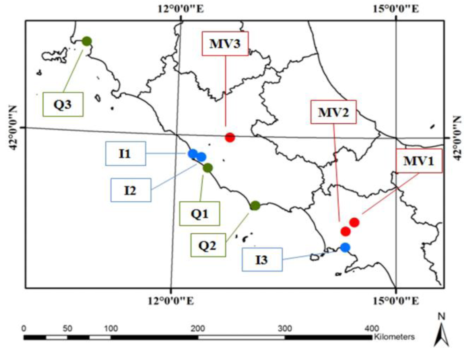
The study area is located in central Italy, where different images and field spectra were acquired. Highways, secondary roads and parking lots were the object of study. Airports, too, were included, particularly in view of the need for asphalt areas with similar alteration conditions and level of bitumen coverage, not to mention big enough to be recognized in images.

Hyperspectral and multispectral images were acquired in Central Italy during the period 2007–2010 as follows: MIVIS images of Caserta (MV1), Napoli (North) (MV2) and Guidonia (MV3); Quickbird images of Pratica di Mare (Q1), Sabaudia (Q2) and Follonica (Q3) and, finally, Ikonos imagery of Fiumicino (I1), Acilia (I2) and Napoli (East) (I3) (

Table 1. Geographic location of study areas: Caserta (MV1), Napoli (North) (MV2) and Guidonia (MV3); Quickbird images of Pratica di Mare (Q1), Sabaudia (Q2) and Follonica (Q3) and, finally, Ikonos imagery of Fiumicino (I1), Acilia (I2) and Napoli (East) (I3) MIVIS, Multispectral Infrared and Visible Imaging Spectrometer.

	Data	Location	Imagery
	MIVIS	Caserta	MV1
		Naples (North)	MV2
		Guidonia	MV3
	Quickbird	Pratica Di Mare	Q1
		Sabaudia	Q2
		Follonica	Q3
	Ikonos	Fiumicino	I1
		Acilia	I2
		Naples (East)	I3

). MIVIS imagery was acquired during the 2009 and 2010 field campaigns relevant to the National Operative Program (PON) 2007–2013 (“Security for the Development of Southern Italy” mission).

2.2. Field Data

To analyze the main features of paved surfaces that could be derived by images, during field surveys, descriptive data and spectra of asphalt surfaces were acquired. Spectral signatures with different bitumen coverage levels were selected in main roads and parking lots. The surfaces analyzed during the field surveys were aged from 1 to 5 years old, with different conditions and distress. The newest pavements were observed in only a few locations.

Spectroradiometrical data were acquired using a Fieldspec 3 (A.S.D., Boulder-Colorado) that measures the light intensity in a wavelength range between 350 and 2500 nm, through an optical fiber bundle that collects the reflected radiation with a 25° conical field of view. The spectroradiometer was set at reflectance mode, and a Spectralon panel (high-density fluoropolymer), assumed as a Lambertian surface, was used as the white reference. The radiometer was positioned at 67 cm to the target to cover a measured area of about 700 cm². For each target, representative spectra were calculated, averaging 10 spectral signatures (the result of 10 acquisition cycles). Using the procedure of [15], principal features, such as color, particle size, grain morphology and the percentage of inert substance covered by bitumen, were analyzed in addition to asphalt spectra. About 500 different targets were acquired and integrated into a spectral library and GEO database.

The percentages and dimensions of aggregates can vary considerably; thus, dissimilar surface characteristics and radiometric responses are possible. For the dimensional analysis of aggregates, ANAS (Azienda Nazionale Autonoma delle Strade (Italian National Roads Department)) Technical Notes (2009) were followed. For granulometric analysis, [22] was considered, taking into account only classes between coarse gravel (32–16 mm) and very fine sand (0.125–0.062 mm). For grain roundness analysis, a comparative chart [23], commonly used in sedimentological analysis, was adopted. For aggregate lithology, only 4 kinds of useless aggregate, such as carbonate, silicate and recycled material (material derived from crushing man-made structures), were considered. Finally, asphalt colors were evaluated using the Munsell (M) gray scale (10 classes) [24].

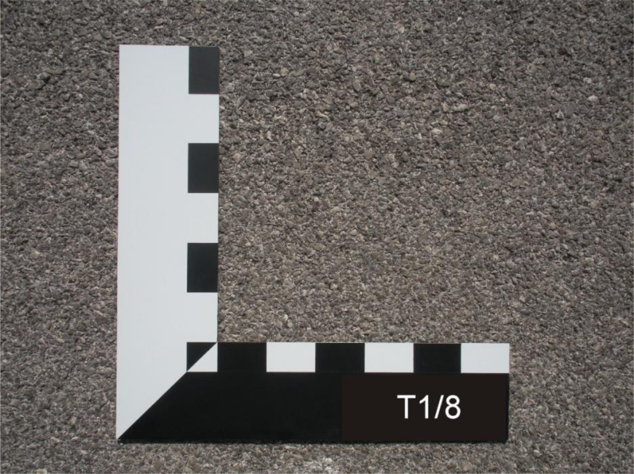
To validate asphalt field characteristics, digital photos were acquired with a Nikon Coolpix S560. To guarantee comparability pictures, a 40 cm × 40 cm reference ruler (consisting of 5 cm of white and black color reference stripes) was used (Figure 1).

Considering different field light conditions, the white normalization tool on the digital camera was used to obtain comparable pictures. This camera setting ensures a more accurate ground reference.

As the bitumen film on an asphalt surface significantly influences the radiometric response, 5 classes of “bitumen percentage” (from 0%–20% to 80%–100%) were defined, readapting [25] sedimentological microscopic analysis, to describe this presence over the aggregate surface. All information collected in the field was integrated in a GEO database, whereby the large amount of data could be handled efficiently.

2.3. Laboratory Data

Most papers on asphalt characteristics studies underline the necessity for laboratory tests. Similar to a laser scanner [26] or digital imaging processing [27,28], used respectively for texture characteristics and sample strain evaluation, spectroradiometrical laboratory measurements can be computed to analyze asphalt physical properties for remote sensing applications.

It was not possible to recognize in images and, consequently, to obtain samples of new/fresh asphalts from the studied areas. Thus, new lab samples were made according to ANAS technical specifications. Hence, it was possible to investigate the relationship between wavelengths of 460 nm and 740 nm, as well as the existence of the asphalt line.

As stated, bitumen presence on asphalt surfaces is directly correlated to removal processes and permits some differentiations to be made. Asphalt samples, related to hot mixed asphalt (HMA), were prepared in the laboratory, and spectroradiometer measurements were performed. Each sample compound had known physical characteristics, including saturated surface dried particle density (EN 1097-6 (g/cm³)), water absorption (%) (EN 1097-6) and aggregate and mixture grading (%).

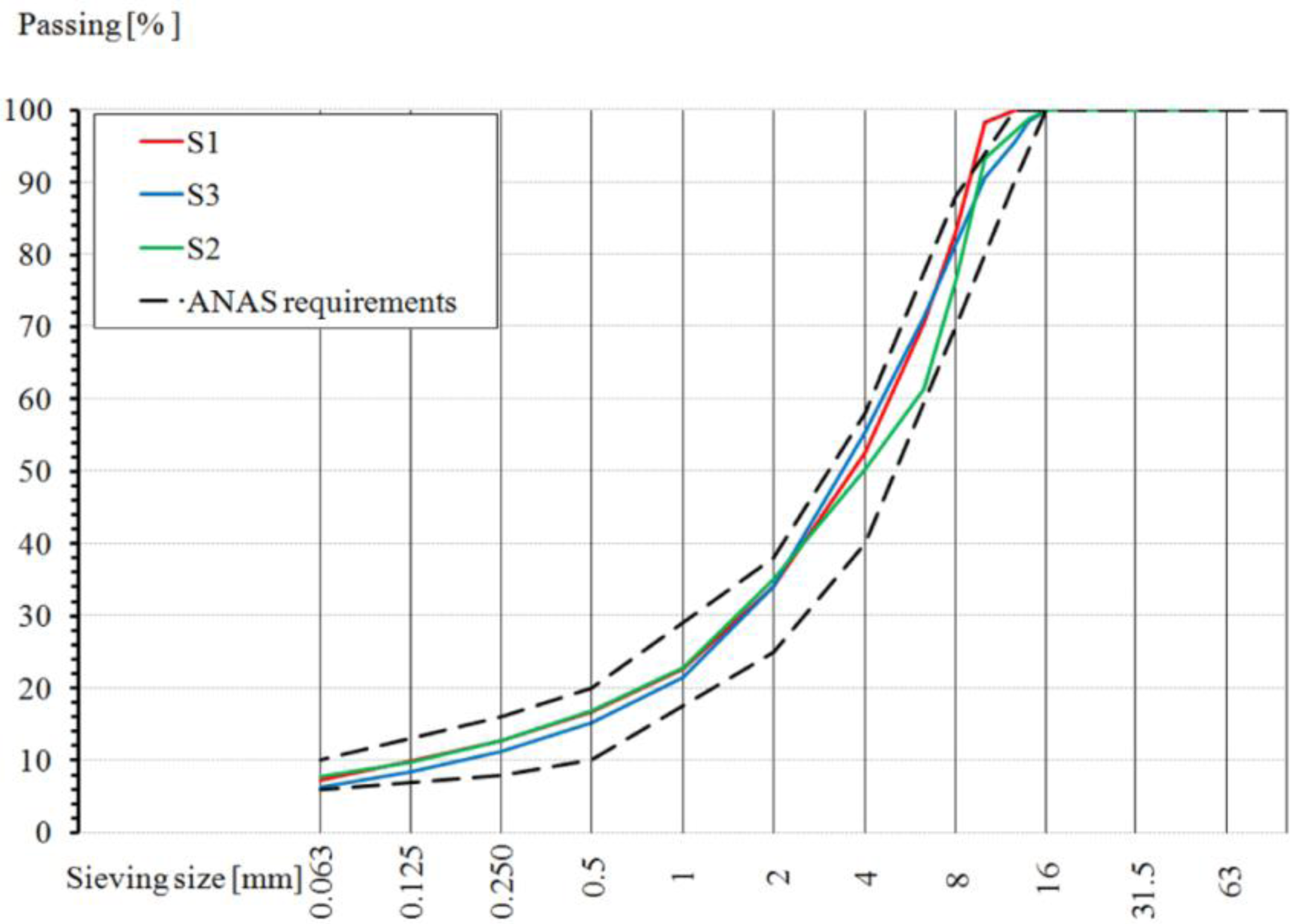
For this experiment, different samples were used. Generally, asphalt surfaces are composed of silicate materials, such as basalts. Thus, leucititic tephrite aggregates were used, to evaluate differences in the relationship between spectral signatures. Three mixtures (S1, S2 and S3) of a binder and a top layer of a paved surface were performed by melting different percentages of dense sand (0–5 cm), fine dense gravel (2–6.3 cm), dense gravel (5–11 cm) and filler. For each of these compositions different percentages of bitumen were added. Some 46 asphalt samples to be compacted according to the Marshall method and ANAS requirements (Figure 2) were obtained. For all samples, bitumen content ranged between 3.9% and 6.5%.

Spectroradiometric measurements were carried out on compacted samples under controlled laboratory conditions. Spectral signatures were acquired using the Spectralon panel as the white reference and a 50 watt Pro-Lamp as a light source. Each measurement was performed with 50 integration cycles to minimize the light oscillations, while, to minimize the scattering effects due to sample roughness, spectra were collected, rotating each sample by 90°, and the mean value was computed.

2.4. Remotely-Sensed Data

MIVIS images were acquired at a flight altitude of 1500 m above sea level corresponding to a 3 m × 3 m ground pixel size. Images, taken in the summer in Central Italy were composed of 3 distinct runs of variable length, from 5 to 30 km.

MIVIS is an airborne modular instrument consisting of 4 spectrometers. These simultaneously measure the radiation from the Earth’s surface in the visible (20 bands between 430 and 830 nm), near (8 bands between 1150 and 1550 nm), medium (64 bands between 2000 and 2500 nm) spectra and the thermal infrareds (10 bands between 8200 and 12,700 nm) for a totality of 102 bands. It is characterized by an IFOV (instantaneous field of view) of 2 mrad and an FOV (field of view) of 71°.

To enlarge the study of remotely-sensed images with a lower spectral resolution, Quickbird and Ikonos multispectral data were considered. Quickbird and Ikonos sensors are composed of 4 bands in the visible and near infrared range (blue, green, red and NIR) and a panchromatic band (450–900 nm). The spatial resolutions of images are, respectively, 2.8 m/4.0 m in multispectral mode and 0.7 m/1.0 m in panchromatic mode at nadir.

3. Data Computation

3.1. Field Data Computation

In the 350–2500 nm wavelength range, asphalt reflectance is generally very low and dominated by the presence of bitumen, which almost totally absorbs the incident solar radiation. It is only after aging and degradation processes, causing the loss of the bitumen component and the outcropping of aggregate, that the reflectance values slightly increase and the absorption peaks related to mineralogical characteristics of outcropping aggregate fragments appear. Therefore, asphalt color can be used to identify variations from quality requirements [21–29].

About 40 spectra for each Munsell grey-scale class were considered, except for the first 3 color classes, where the number of targets, in studied areas, decreases significantly (M3 (25), M2 (18) and M1 (9)). This was mainly due to the difficulty of identifying newer paved areas. Generally, classes with low values of the bitumen percentage correspond to the last Munsell color class (M8 and M9), despite high values of bitumen corresponding to low Munsell color classes (M1 and M2). 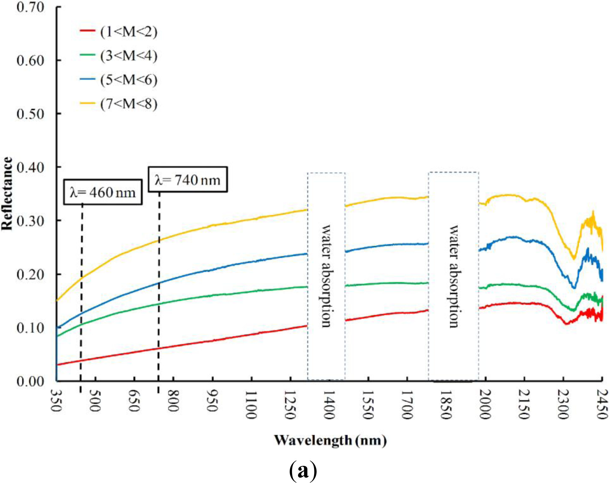According to [19], this observation implies that paved surface alteration is closely related to the decrease of bitumen on the aggregate surface and, consequently, to colorimetric changes. To assess bitumen coverage levels between paved surfaces in remotely-sensed images, field asphalt spectra were analyzed. The analysis of field spectral data of asphalt, free of damage and distress in the Vis and NIR range, showed that reflectance values at λ = 460 nm and λ = 740 nm can be used to describe differences in asphalt surfaces. Considering reflectance values at these two wavelengths, the differences among asphalts was evident: new road surfaces, dominated by hydrocarbon absorptions, have reflectance values lower than older surfaces, in turn dominated by mineral signals. Considering that the change of slope in the Vis spectral region could be matched to the bitumen removal processes (Figure 3a), the reflectance values at λ = 460 nm and λ = 740 nm were represented in a scatter plot. The reflectance values of asphalt pixels group together as an asphalt macro-class, showing a linear distribution (|y = αx + b|) that can be assumed to be an “asphalt line”. To facilitate imagery classification processes, Munsell color classes were grouped into 4 main clusters (asphalt sub-classes), each composed of 2 color classes, as follows: Class 1: 1 < M < 2; Class 2: 3 < M < 4; Class 3: 5 < M < 6; and Class 4: 7 < M < 8 (Figure 3b). Classes 9 and 10 were not present or significant (ex. painted asphalts) in the studied areas.

Field spectra collected in each study area were used to compute the slope coefficients (α) and b coefficients of the equation for each area. The slopes of these asphalt lines showed values between 0.6 and 0.8 and b terms close to zero; the R-squared of these regression lines is always greater than 0.9.

3.2. Laboratory Data Computation

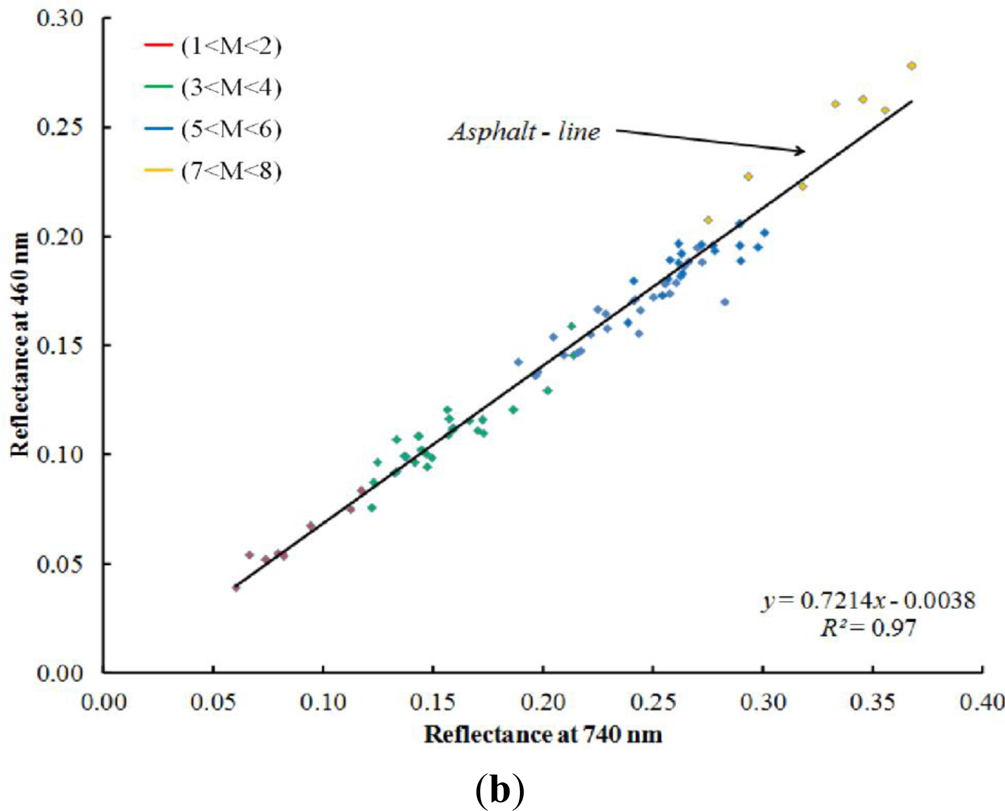
To investigate whether the relationship between reflectance values at 460 nm and 740 nm could be assessed, laboratory spectral measurements were made on 46 specially prepared bituminous mixtures of new asphalt samples. These can be referred to as Class 1 < M < 2. Samples were prepared taking into account technical specifications for the road management of the investigated districts.

As stated, the newest asphalts were investigated in the laboratory. Due to their rapid alteration and/or bitumen removal, their presence in the field is limited. These analyses were then computed to ensure the linear regression validity for this kind of very new (fresh) asphalts.

These kinds of targets were melted homogenously and not subjected to weather or superficial degradation. The analysis of spectra confirm, as for field data, that reflectance values and the slopes of spectral signatures in the Vis region decrease as the bitumen content increases. This suggests the retrieval of bitumen percentage. By calculating the spectral signature standard deviation, the largest differences in bitumen content can be pointed to. In Figure 4a substantial variation in bitumen percentage by dry weight of aggregate is highlighted by the distant among the curves (e.g., ΔS1-1_a–d = 1.94%). For low delta values, too, in mixtures ΔS1-2_a–d (1.38) and ΔS1-3_a–d (1.46), the spectral signatures are separable; however, the negative bitumen percentage that is detectable with spectral measurements cannot be established.

As was noted in the field data, in the spectrum, a slope change corresponding to the variation of bitumen content occurs. This is also seen in lab spectra: in the Vis region, when the bitumen percentage increases, the slope of the spectral signatures decreases, and their shape generally switches from a ramp to a flat geometry. This shape variation due to the bitumen presence on the surface has already been pointed out [30] and correlated with the early stages of surface alteration [11–15].

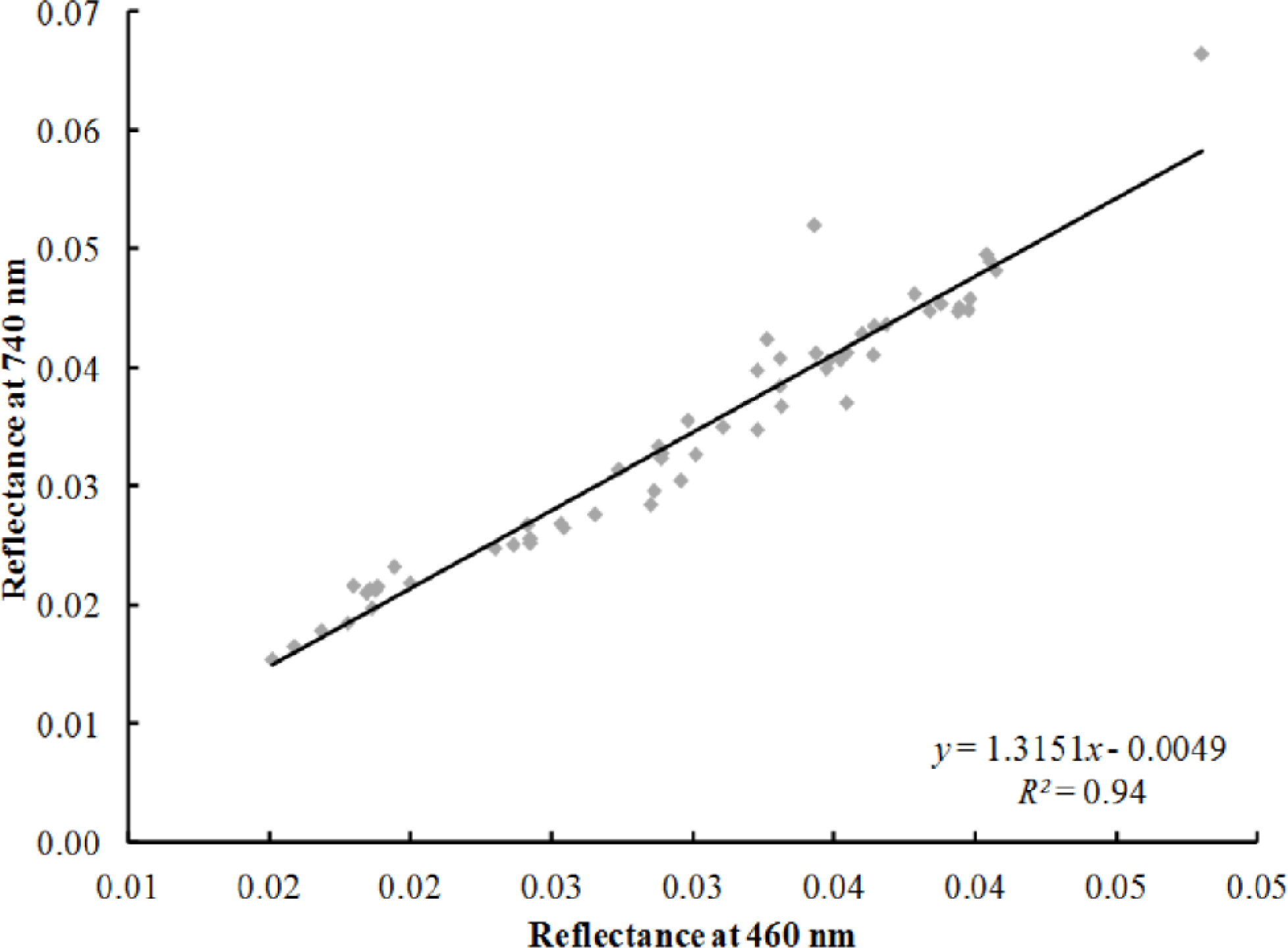
To investigate the relationship between 460 nm and 740 nm, all spectral signatures were analyzed by a scatter plot analysis. The results provide a linear correlation with an R-squared of 0.94 (Figure 5) and show that the asphalt line can also be derived for fresh asphalts.

3.3. Image Classification

The challenge of this research was to discriminate between different HMA asphalt classes using remotely-sensed images. By integrating both laboratory and field data, the asphalt level of the bitumen coverage could be better determined and, hence, the different surfaces, too.

3.3.1. Methodology

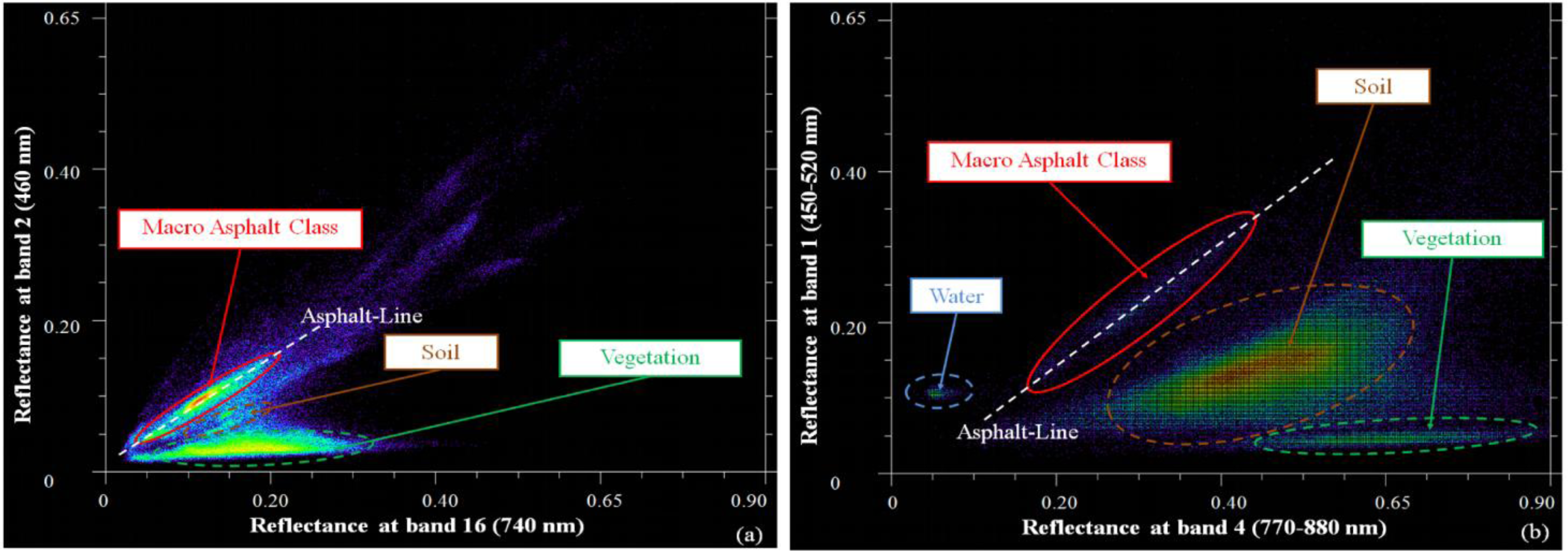
Both hyperspectral (MIVIS) and multispectral (Quickbird and Ikonos) data were analyzed to integrate field observations with remote sensing imagery. Before applying image classification procedures, a preliminary analysis of single MIVIS bands, corresponding to a spectral range of 400 nm–870 nm, was performed. This wavelength range facilitates the comparison between hyperspectral and multispectral imagery. Taking into account the field spectral signatures, scatter plots with MIVIS Bands 2 (λ = 460 nm) and 16 (λ = 740 nm) were computed.

Figure 6a shows that pixels corresponding to asphalted surfaces were grouped essentially in a single area. This corresponds to the asphalt macro-class previously identified with field data. Thus, it was possible to effectively discriminate between different asphalted surfaces within images, even at this preliminary step of image pre-processing aimed at ROI detection. In the scatter plot, pixels corresponding to vegetated areas and soils were well clustered in different groups (Figure 6a).

Scatter plot analysis was also conducted for Quickbird and Ikonos images using Bands 1 (450 nm–520 nm) and 4 (760 nm–890 nm), which best approximate wavelengths λ = 460 nm and λ = 740 nm. It emerged that the cluster of pixels referring to paved surfaces had the same distribution, even if their spectral ranges were significantly larger than those for MIVIS (Figure 6b).

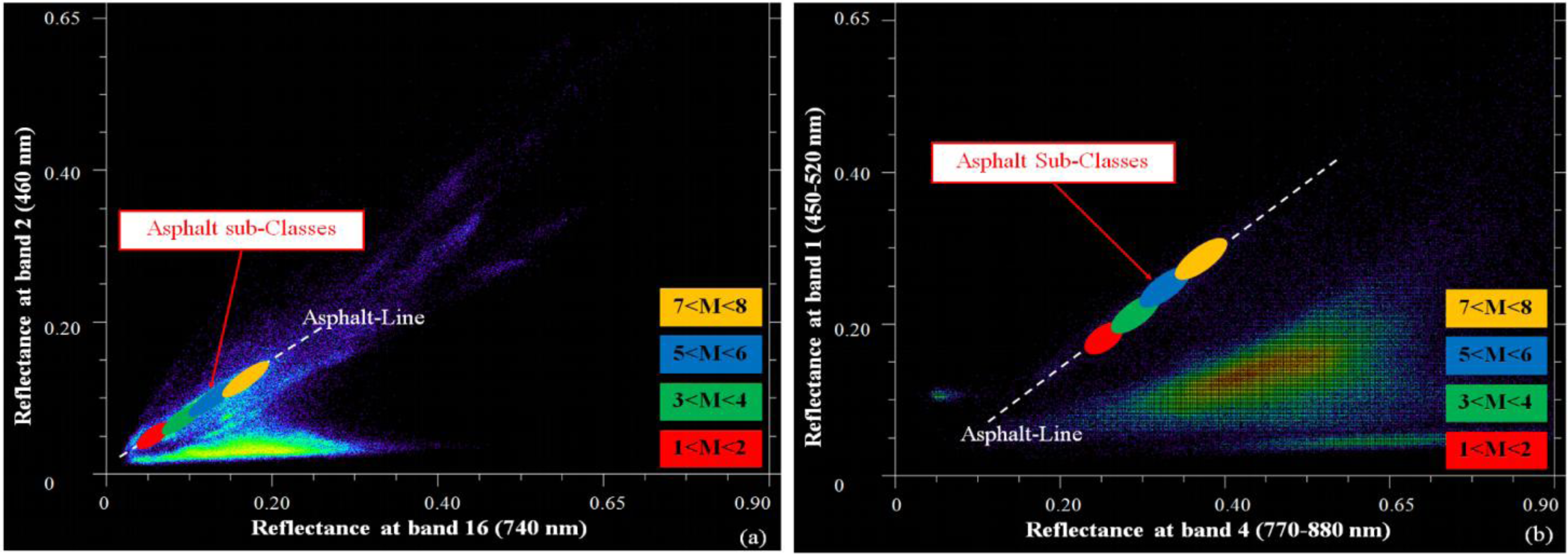
Moreover, taking into account field observations, in image scatter plots, clusters were recognized corresponding to the Munsell (M) scale (Class 1: 1 < M < 2; Class 2: 3 < M < 4; Class 3: 5 < M < 6; and Class 4: 7 < M < 8) (Figure 7).

The SAM algorithm was selected to classify asphalt surfaces according to their bitumen removal process, given that this is insensitive to illumination and suitable for homogeneous areas.

Spectral Angle Mapper classification is based on a comparison of the spectral image with a reference spectrum (endmembers or spectral libraries) and it evaluates spectra similarity in order to accentuate the target characteristics. This method treats both spectra as vectors and calculates the spectral angle between them. In fact, SAM attempts to obtain the angles (α) (between 0 and π/2) formed between reference and image spectrum Equation (1), treating them as vectors in a space with N-dimensionality equal to the number, N, of bands [31].

Angles were calculated by applying the following formulation:

$$\alpha =\frac{{\text{cos}}^{-1}\sum {\tau }_1{\tau }_2}{\sqrt{\sum {\left({\tau }_1\right)}^2\sum {\left({\tau }_2\right)}^2}}$$

(1)

where:

τ1	is the image spectrum
τ2	is the reference spectrum

To reduce noise and the computational requirements for subsequent processing [32], a Minimum Noise Fraction Transformation (MNF) was applied to the images. The MNF transformation produces principal components and normalizes the eigenvalues relative to the variance of the sensor noise estimate [33,34]. After a preliminary ROI-selection step, based on field surveys and image interpretation in a scatter plot analysis, a Pixel Purity Index (PPI) was computed. PPI locates the purest pixels in the ROIs to better identify endmember spectra to be used in the SAM algorithm [31]. The SAM method uses the vector direction of spectral signatures, and a threshold value must be selected as a variable to perform a classification. The asphalt line angular coefficients, corresponding to each analyzed image, were used as the threshold. For both hyperspectral (Figure 8) and multispectral images (Figure 9) the same procedure was adopted.

Confusion matrices were computed to retrieve the overall accuracy and the kappa-coefficient [35,36]. The overall accuracy and the kappa-coefficient (κ) measure the accuracy of the classification. The overall accuracy is computed by dividing the total number of correctly classified pixels by the total number of reference pixels [37]. The kappa-coefficient (κ) is calculated by Equation (2):

$$\kappa =\frac{\left({\text{P}}_0-{\text{P}}_{\text{c}}\right)}{\left(1-{\text{P}}_{\text{c}}\right)}$$

(2)

where P₀ is the proportion of units where there is agreement with the ground-truth and P_c is the proportion of units that would be expected to agree by chance [38,39]. If there is complete agreement with the ground-truth, then κ = 1, while no agreement is related to κ ≤ 0.

3.3.2. Classification

To extrapolate the linear equation corresponding to the asphalt line, spectral signatures corresponding to each pixel were extracted from the images. These were exported as an ASCII file and processed to extrapolate reflectance values corresponding to selected bands.

For MIVIS images, the angular coefficients (α) of asphalt lines ranged from 0.64 and 0.86, while for Ikonos and Quickbird (

Table 2. Asphalt line angular coefficients.

Data	Imagery
	MIVIS			Quickbird			Ikonos
	MV1	MV2	MV3	Q1	Q2	Q3	I1	I2	I3
α	0.64	0.65	0.86	0.85	0.63	0.79	0.75	0.63	0.74
R2	0.97	0.94	0.97	0.94	0.91	0.95	0.93	0.95	0.97

), these values varied from 0.63 to 0.85. As field data, the b coefficients were about 0 for all the asphalt lines.

All 4 asphalt sub-classes were well represented in the images, such as for densely urbanized or rural areas and airports. These classes were then used in the supervised classification procedures applied to the images. The Spectral Angle Mapper classifier was applied to each image; angular coefficients of asphalt line, corresponding to each analyzed image, were used as the threshold value.

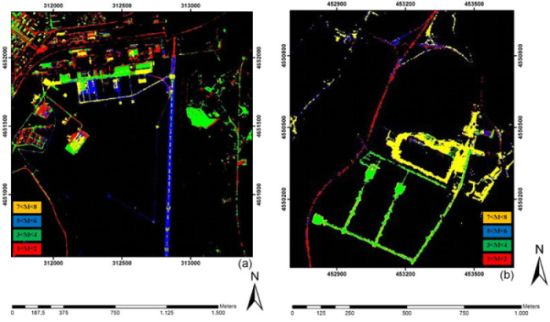
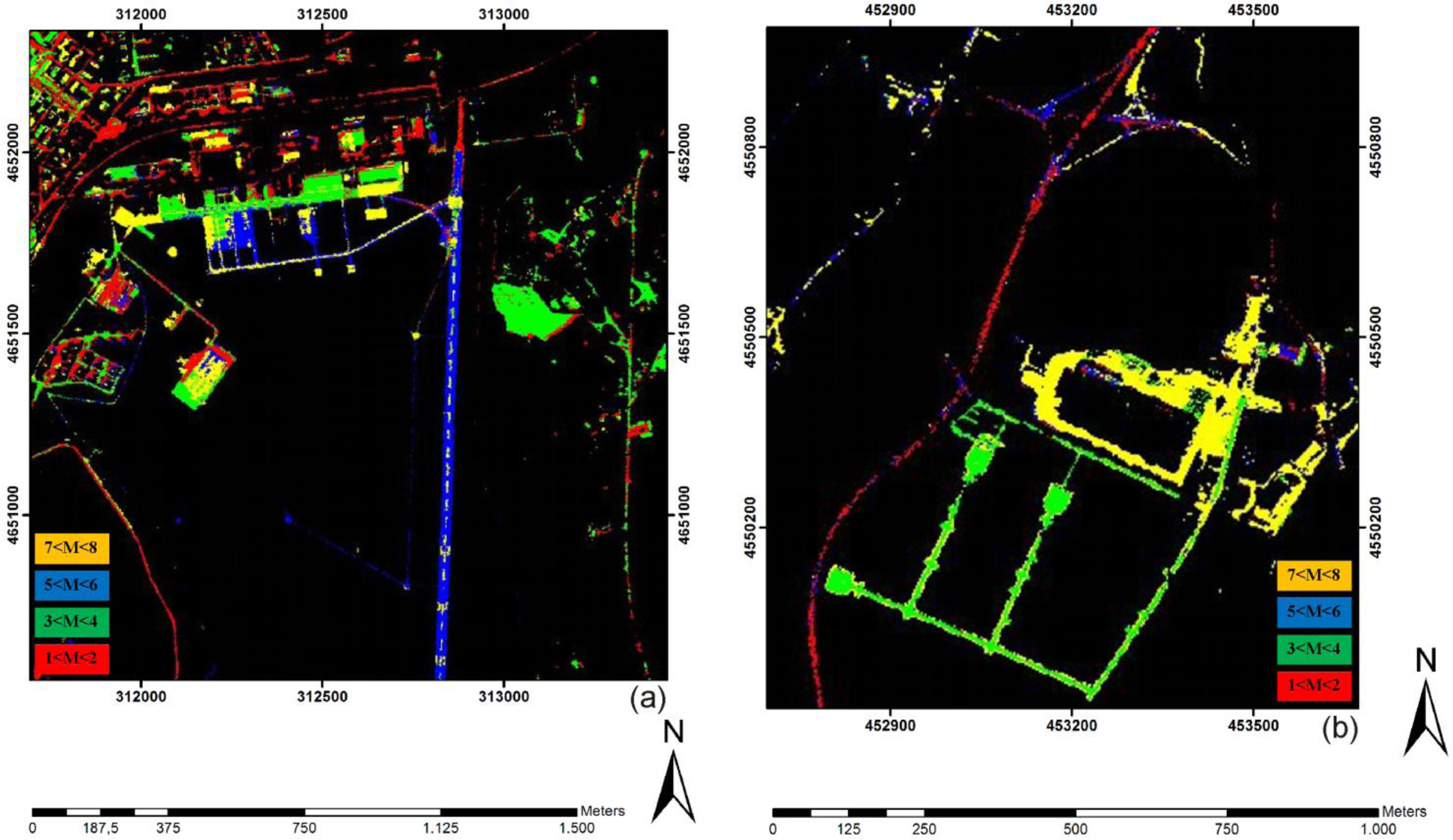
Figure 8a presents the MIVIS classification of Guidonia airport and the surrounding urban. A commercial area near Caserta City is shown in Figure 8b.

In both figures, the new parking lot with a lower level of the bitumen coverage, corresponding to Class 2: 3 < M < 4, is green. New roads are red (Class 1: 1 < M < 2), and parking lots with the lowest bitumen coverage are yellow; Class 3: 5 < M < 6 is blue and corresponds to a landing strip.

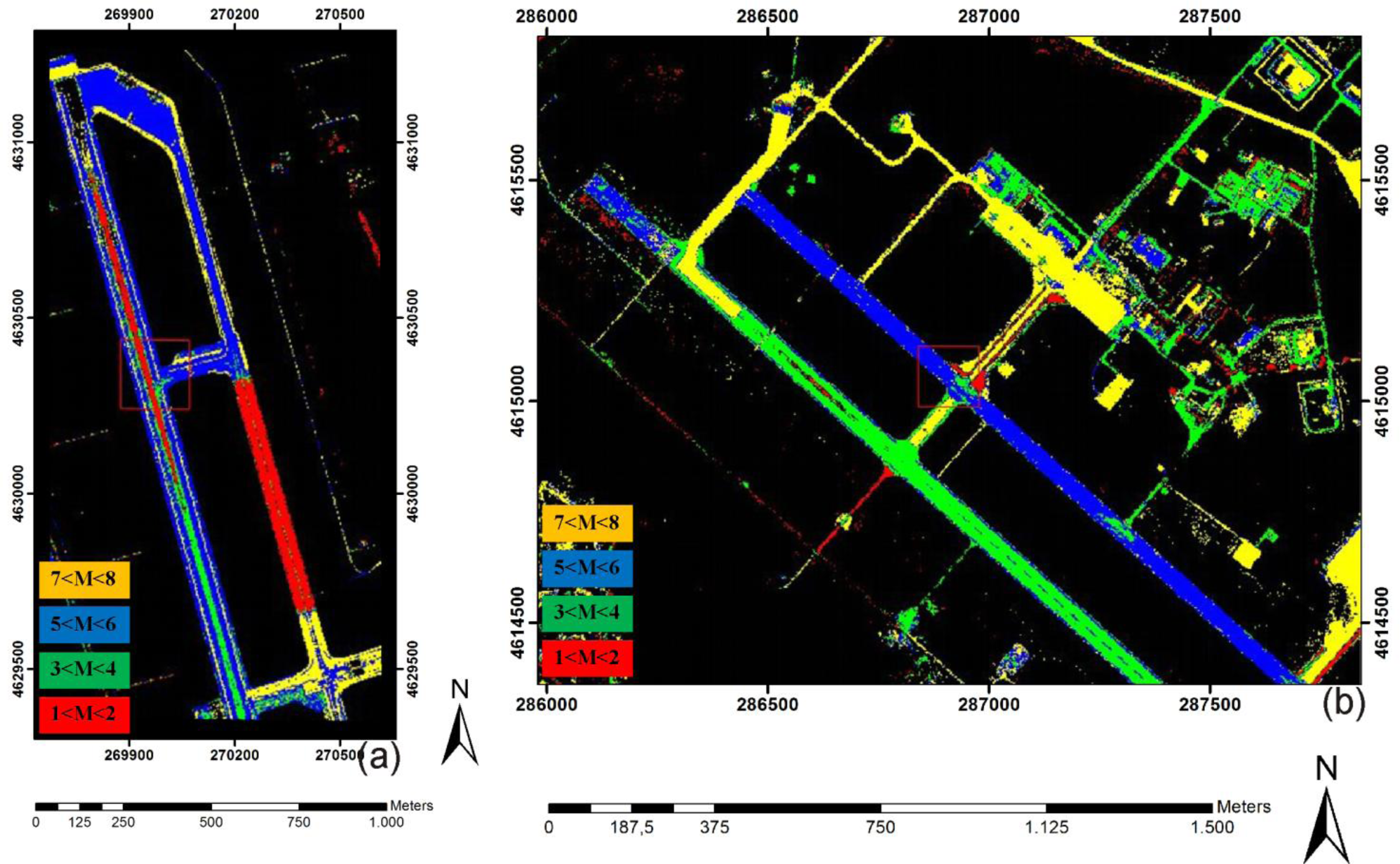
Figure 9 shows that the classification of satellite images here, too, are the landing strips composed of Class 3 (5 < M < 6; blue).

In Pratica di Mare airport (Figure 9b) Class 2 (3 < M < 4; green) can be identified in a secondary landing strip. Class 1 (1 < M < 2; red) appears only in a limited number of areas, even though in Figure 9a, a new asphalt spread can be observed in a secondary landing strip. Parking lots are usually areas with a low degree of bitumen coverage or aged asphalt Class 4 (7 < M < 8; yellow) (e.g., plane parking lots of the Pratica di Mare airport).

4. Results and Discussion

Based on the same criteria used to select ROIs for the SAM classification, the validation ROI dataset was created to access the classification accuracy for each image. Confusion matrices were used to retrieve overall accuracy and the kappa-coefficient.

The classifications obtained for the 3 MIVIS images present an overall accuracy (OA) between 90.5% and 93.4% and a κ-coefficient (κ) between 0.87 and 0.91. Classification results obtained for satellite images present an accuracy between 93.7% and 98.1% (0.92 < κ < 0.97) for Quickbird data and between 90.8% and 95.0% for Ikonos (0.88 < κ < 0.92). These are reported in

Table 3. MIVIS, Quickbird and Ikonos classifications results.

Data	Imagery
	MIVIS			Quickbird			Ikonos
	M1	M2	M3	Q1	Q2	Q3	I1	I2	I3
OA(%)	91.35	90.48	93.42	97.74	93.71	98.08	95.00	90.83	94.26
κ	0.88	0.87	0.91	0.97	0.92	0.97	0.93	0.88	0.92

.

In all nine images’ confusion matrices, unclassified pixels are rare and commission errors are about 5% for Quickbird and 10% for MIVIS and Ikonos. This may be traced to the similar pixel spatial resolution. The smaller spectral resolution of Quickbird and Ikonos sensors does not appear to influence the accuracy of asphalt classes. Nevertheless, both sensors detect asphalt pavement using the asphalt line angular coefficient as the threshold in the Spectral Angle Mapper classifier.

5. Conclusions

Recent advances in our knowledge of the spectral behavior of asphalt supports its use as calibration and validation targets for imagery atmospheric corrections or for innovative applications in civil engineering. As differentiation procedures are particularly challenging, most authors emphasize the need to associate supplementary field and laboratory analysis. This paper analyses field and laboratory spectral signatures of asphalt to improve its differentiation and correlation with hyperspectral and multispectral imagery. The analysis of field spectral signatures shows a significant change of slope in the visible and near-infrared region of the spectra. This can be linked to the loss of superficial bitumen. Using reflectance values at λ = 460 nm and λ = 740 nm, scatter plots reveal a good grouping of pixels, which could be related to an asphalt macro-class. This linearly distributed clustering can be referred to an interpolated line assumed as an asphalt line. Referring to the Munsell (M) color chart, four main clusters are identified as asphalt sub-classes. Field spectra are used to compute the equation of the asphalt line for each area, and the angular coefficients (α) show values from 0.6 to 0.8. The subsistence of the asphalt line is also confirmed for laboratory fresh asphalt (R² = 0.94), which can be referred to the non-degraded targets. For asphalt line detection on remotely-sensed images, MIVIS Bands 2 and 16 and Ikonos and Quickbird Bands 1 and 4 are selected considering their best approximation with the field and lab wavelength (λ = 460 nm and λ = 740 nm). To identify pixels related to paved surfaces, interpolation lines of asphalt are calculated, and their angular coefficients are used as threshold values in a SAM algorithm. Asphalt line angular coefficients retrieved from remotely-sensed images reveal similar values. Values range from 0.64 and 0.86 for MIVIS imagery and between 0.63 to 0.85 for Ikonos and Quickbird. Regarding field data, the b coefficients were about zero for all the asphalt lines. This analysis showed that the pixel cluster for paved surfaces had the same distribution in the field, lab and remotely-sensed images, even though their spectral and spatial resolutions are different. The application of these threshold values in the Spectral Angle Mapper algorithm shows high overall accuracies: MIVIS images present values of about 91.8%, which are comparable with those obtained for Quickbird (an averaged accuracy of 96.5%) and Ikonos (an averaged accuracy 93.3%). The proposed procedure reduces the processing time to retrieve a threshold value to be used in A Spectral Angle Mapper classification for asphalt studies. By deriving threshold values from asphalt lines, it is possible to avoid the iterative procedures typical of this classification method.

Classification results showed that both hyperspectral and multispectral imagery can supply local government authorities with a tool to locate asphalt pavements that need to be checked for maintenance and to improve road monitoring policies or to update the road registry. The detection of bitumen removal effects by remote sensing analysis could be an indicator for other phenomena, such as friction reduction and bitumen concrete aging. Furthermore, the possibility of differentiating asphalts, relating to their spectral variability, may be an important tool to improve their usage in image calibration and validation procedures. Additional laboratory spectral measurements of different asphalt pavements (SMA, PMA, macadam, etc.) will be necessary to extend remote sensing analysis. Although it is still impossible to substitute in situ inspections to define asphalt distress levels, remote sensing techniques can limit time-consuming field surveys. Moreover, new technologies, such as unmanned aerial vehicles (UAV) with ad hoc sensors, designed for the same wavelengths used in this paper, can be used in effective road monitoring.

References

- Themistocleous, K.; Hadjimitsis, D.G.; Retalis, A.; Chrysoulakis, N.; Michaelides, S. Precipitation effects on the selection of suitable non-variant targets intended for atmospheric correction of satellite remotely sensed imagery. Atmos. Res 2012, 131, 73–88. [Google Scholar]
- Gao, B.C.; Montes, M.J.; Davis, C.O.; Goetz, A.F.H. Atmospheric correction algorithms for hyperspectral remote sensing data of land and ocean. Remote Sens. Environ 2009, 113, 17–24. [Google Scholar]
- Karpouzli, E.; Malthus, T. The empirical line method for the atmospheric correction of IKONOS imagery. Int. J. Remote Sens 2003, 24, 1143–1150. [Google Scholar]
- Vassilakis, E. Remote sensing of environmental change in the Antirio Deltaic Fan region, Western Greece. Remote Sens 2010, 2, 2547–2560. [Google Scholar]
- Novack, T.; Esch, T.; Kux, H.; Stilla, U. Machine learning comparison between worldview-2 and quickbird-2-simulated imagery regarding object-based urban land cover classification. Remote Sens 2011, 3, 2263–2282. [Google Scholar]
- Wang, C.; Hu, Q.; Lu, Q. Research on a novel low modulus OFBG strain sensor for pavement monitoring. Sensors 2012, 12, 10001–10013. [Google Scholar]
- Skoglar, P.; Orguner, U.; Tornqvist, D.; Gustafsson, F. Road target search and tracking with gimballed vision sensor on an unmanned aerial vehicle. Remote Sens 2012, 4, 2076–2111. [Google Scholar]
- Mohammadi, M. Road classification and condition determination using hyperspectral imagery. Int. Arch. Photogramm. Remote Sens. Spatial Inf. Sci 2012, XXXIX-B7, 141–146. [Google Scholar]
- Italos, C.; Hadjimitsis, D.G.; Alexakis, D.D.; Themistocleous, K.; Agapiou, A.; Nisantzi, A.; Papoutsa, C.; Papadavid, G. Integrated Use of Satellite Remote Sensing and GIS for the Development of a Sophisticated Sustainability Index for Urban Areas: A Case Study of Paphos City (Cyprus). In Proceedings of the 32nd EARSeL Symposium Advances in Geosciences, Mykonos Island, Greece, 21–24 May 2012; pp. 587–593.
- Gomez, R.B. Hyperspectral imaging: A useful technology for transportation analysis. Opt. Eng 2002, 41, 2137–2143. [Google Scholar]
- Herold, M.; Roberts, D.A.; Gardner, M.E.; Dennison, P.E. Spectrometry for urban area remote sensing-development and analysis of a spectral library from 350 to 2400 nm. Remote Sens. Environ 2004, 91, 304–319. [Google Scholar]
- Andreou, C.; Karathanassi, V.; Kolokoussis, P. Investigation of hyperspectral remote sensing for mapping asphalt road conditions. Int. J. Remote Sens 2011, 32, 6315–6333. [Google Scholar]
- Herold, M.; Roberts, D.; Noronha, V.; Smadi, O. Imaging spectrometry and asphalt road surveys. Transp. Res. Part C: Emerg. Technol 2008, 16, 153–166. [Google Scholar]
- Pascucci, S.; Bassani, C.; Palombo, A.; Poscolieri, M.; Cavalli, R. Road asphalt pavements analyzed by airborne thermal remote sensing: Preliminary results of the venice highway. Sensors 2008, 8, 1278–1296. [Google Scholar]
- Mei, A.; Salvatori, R.; Allegrini, A. Analysis of paved areas with field data and MIVIS hyperspectral images. Ital. J. Remote Sens 2011, 43, 147–159. [Google Scholar]
- Mei, A.; Salvatori, R. Urban mapping using IKONOS imagery. Int. J. Remote Sens. Geosci 2013, 2, 55–58. [Google Scholar]
- Lin, X.; Liu, Z.; Zhang, J.; Shen, J. Combining multiple algorithms for road network tracking from multiple source remotely sensed imagery: A practical system and performance evaluation. Sensors 2009, 9, 1237–1258. [Google Scholar]
- Cavalli, R.M.; Fusilli, L.; Pascucci, S.; Pignatti, S.; Santini, F. Hyperspectral sensor data capability for retrieving complex urban land cover in comparison with multispectral data: Venice city case study (Italy). Sensors 2008, 8, 3299–3320. [Google Scholar]
- Herold, M.; Roberts, D.A. Spectral characteristics of asphalt road aging and deterioration: Implications for remote-sensing applications. Appl. Opt 2005, 44, 4327–4334. [Google Scholar]
- Cloutis, A.E. Spectral reflectance properties of hydrocarbons: Remote-sensing implications. Science 1989, 245, 165–168. [Google Scholar]
- Claine, P.J. Chemical Composition of Asphalt as Related to Asphalt Durability, 1st ed.; Transportation Research Record: Washington, DC, USA, 1984. [Google Scholar]
- Wentworth, C.K. A scale of grade and class terms for clastic sediments. J. Geol 1922, 30, 377–392. [Google Scholar]
- Powers, M.C. A new roundness scale for sedimentary particles. J. Sediment. Petrol 1953, 23, 117–119. [Google Scholar]
- Munsell, A.H. A pigment color system and notation. Am. J. Psychol 1912, 23, 236–244. [Google Scholar]
- Shvetsov, M.S. Concerning Some Additional Aids in Studying Sedimentary Formations; Moscow University Bulletin: Moscow, Russia, 1954; Volume 29, pp. 61–66. Available online: http://msupublishing.ru/index.php?option=com_content&view=article&id=356&Itemid=100123 (accessed on 21 March 2014).
- Bitelli, G.; Simone, A.; Girardi, F.; Lantieri, C. Laser scanning on road pavements: A new approach for characterizing surface texture. Sensors 2012, 12, 9110–9128. [Google Scholar]
- Bruno, L.; Parla, G.; Celauro, C. Image analysis for detecting aggregate gradation in asphalt mixture from planar images. Construct. Build. Mater 2012, 28, 21–30. [Google Scholar]
- Bessa, I.S.; Castelo Branco, V.T.F.; SOARES, J.B. Evaluation of different digital image processing software for aggregates and hot mix asphalt characterizations. Construct. Build. Mater 2012, 37, 370–378. [Google Scholar]
- Mack, C. Physical Chemistry, Bituminous Materials; Hoiberg, A.J., Ed.; Interscience: New York, NY, USA, 1964; Volume 1. [Google Scholar]
- Mei, A.; Fiore, N.; Salvatori, R.; D’Andrea, A.; Fontana, M. Spectroradiometric laboratory measures on asphalt concrete: Preliminary results. Proced. Soc. Behav. Sci 2012, 53, 514–523. [Google Scholar]
- Kruse, F.A.; Lefkoff, A.B.; Boardman, J.B.; Heidebrecht, K.B.; Shapiro, A.T.; Barloon, P.J.; Goetz, A.F.H. The Spectral Image Processing System (SIPS)-interactive visualization and analysis of imaging spectrometer data. Remote Sens. Environ 1993, 44, 145–163. [Google Scholar]
- Small, C. High spatial resolution spectral mixture analysis of urban reflectance. Remote Sens. Environ 2003, 88, 170–186. [Google Scholar]
- Roger, R.E.; Arnold, J.F. Reliability estimating the noise in AVIRIS hyperspectral images. Int. J. Remote Sens 1996, 17, 1951–1962. [Google Scholar]
- Green, A.A.; Berman, M.; Switzer, P.; Craig, M.D. A transformation for ordering multispectral data in terms of image quality with implications for noise removal. IEEE Trans. Geosci. Remote Sens 1988, 26, 65–74. [Google Scholar]
- Stein, A; der Meer, F.V.; Gorte, B. Spatial statistics for remote sensing: Remote sensing and digital image processing. Image Classif. Spectr. Unmix 1999, 1, 185–193. [Google Scholar]
- Jensen, J.R. Introductory Digital Image Processing; Prentice-Hall: Englewood Cliffs, NJ, USA, 1986. [Google Scholar]
- Lillesand, T.M.; Kiefer, R.W.; Chipman, J.W. Remote Sensing and Image Interpretation; Wiley: Hoboken, NJ, USA, 2004. [Google Scholar]
- Congalton, R.G.; Green, K. Assessing the Accuracy of Remotely Sensed Data: Principles and Practices, 1st ed.; Lewis Publishers: Boca Raton, FL, USA, 1999. [Google Scholar]
- Cohen, J.A. Coefficient of agreement for nominal scales. Educ. Psychol. Measur 1960, 20, 37–46. [Google Scholar]
© 2014 by the authors; licensee MDPI, Basel, Switzerland This article is an open access article distributed under the terms and conditions of the Creative Commons Attribution license (http://creativecommons.org/licenses/by/3.0/).