Article

Remote Sensing-Based Biomass Estimation and Its Spatio-Temporal Variations in Temperate Grassland, Northern China

1
Key Laboratory of Agri-Informatics of Ministry of Agriculture, Institute of Agricultural Resources and Regional Planning, China Academy of Agriculture Sciences, Beijing 100081, China
2
Institute of Agricultural Resources and Regional Planning, Institute of Applied Ecology, Chinese Academy of Sciences, Shenyang 110016, China
3
The Geographical Science College, Inner Mongolia Normal University, Hohhot 010022, China
*
Author to whom correspondence should be addressed.
Remote Sens. 2014, 6(2), 1496-1513; https://doi.org/10.3390/rs6021496
Submission received: 28 December 2013 / Revised: 5 February 2014 / Accepted: 9 February 2014 / Published: 19 February 2014

Abstract

:
Grassland biomass is essential for maintaining grassland ecosystems. Moreover, biomass is an important characteristic of grassland. In this study, we combined field sampling with remote sensing data and calculated five vegetation indices (VIs). Using this combined information, we quantified a remote sensing estimation model and estimated biomass in a temperate grassland of northern China. We also explored the dynamic spatio-temporal variation of biomass from 2006 to 2012. Our results indicated that all VIs investigated in the study were strongly correlated with biomass (α < 0.01). The precision of the model for estimating biomass based on ground data and remote sensing was greater than 73%. Additionally, the results of our analysis indicated that the annual average biomass was 11.86 million tons and that the average yield was 604.5 kg/ha. The distribution of biomass exhibited substantial spatial heterogeneity, and the biomass decreased from the eastern portion of the study area to the western portion. The interannual biomass exhibited strong fluctuations during 2006–2012, with a coefficient of variation of 26.95%. The coefficient of variation of biomass differed among the grassland types. The highest coefficient of variation was found for the desert steppe, followed by the typical steppe and the meadow steppe.

1. Introduction

Grassland ecosystems represent 40.5% of the land surface of the Earth [1], and their net primary productivity represents approximately 20% of total terrestrial productivity [2]. Accordingly, grasslands play an important role in global carbon cycling. As an important component of the terrestrial ecosystem of China, grassland ecosystems are not only one of the major ecosystems but also an important contributor to energy exchange, carbon pools and biogeochemical cycles [3]. Grasslands occupy 41.7% of the country’s territory [4]. Biomass is a core component of the terrestrial ecosystem and the foundation of grassland, forest, cropland and other terrestrial ecosystems. Numerous case studies of grassland biomass have documented the increasingly prominent role of grassland ecosystems [58]. However, grasslands in arid and semi-arid regions are facing desertification or degradation caused by human activities and climate change. Accurate measurements of grassland biomass and its temporal and spatial variation are important for the utilization and protection of grassland resources.
The use of remote sensing technology has become the most effective approach to biomass estimation [9,10]. Vegetation indices (VIs) calculated from the reflectances measured by remote sensing can reflect the photosynthetic activity of the vegetation and are therefore increasingly used to monitor grassland biomass [11]. Grassland biomass has been successfully estimated based on the normalized difference vegetation index (NDVI), which is a very widely used indicator [9,1115]. Piao et al. [11] estimated the distribution of carbon stocks in China’s grasslands between 1982 and 1999. They established a satellite-based statistical model using national grassland resource inventory data and AVHRR-NDVI data. In addition, biomass was measured as annual peak standing mass during the period from 1981 to 1988, and NDVI dataset was determined as a 7-year (from 1982 to 1988) averaged growing season NDVI (8 × 8 km). Gaitán et al. [9] used a linear regression to assess the relationships between field data and remote sensing data in Patagonian steppes. The field data were obtained between 2008 and 2012 during the growing season. The remote sensing data included several VIs (e.g., NDVI, difference vegetation index (DVI) and enhanced vegetation index (EVI)) that were averaged based on MOD13Q1 reflectance data (250 m × 250 m) for the full growing season. Gao et al. [16] estimated the aboveground biomass using MODIS time series data and field survey data in Inner Mongolia. The MODIS-NDVI, which represented a 16-day composite with 500 m spatial resolution, was calculated using the average NDVI during July and August. However, the estimation of grassland biomass is restricted by multiple factors, such as the biomass sampling time and the spatial resolution of the remote sensing data. Field sampling data are insufficient, and the stability of models remains limited due to the small number of sampling years. The use of multi-temporal satellite data for measuring interannual changes of grassland biomass in semi-arid steppe environments is common, although the selection of appropriate dates for image acquisition is problematic for estimating grassland biomass [17]. The disparity between remote sensing acquisition dates and field data collection dates can influence the success with which a model can be transferred [18]. Due to differences in the sampling times among various steppe types, the temporal resolution of the time series may be an important consideration in terms of the availability of satellite data for modeling field measurements. Additionally, Mutanga and Skidmore [19] noted that the NDVI is limited by its non-linear response, making it insensitive to differences at very low and high densities. Other VIs have been widely used to estimate vegetation biomass based on remote sensing data, e.g., the EVI [17,20], soil adjusted vegetation index (SAVI) [21,22] and modified soil adjusted vegetation index (MSAVI) [2123]. In addition, the high spatial heterogeneity of biomass among different grassland types affects the estimation accuracy of biomass if the same model is used in multiple regions. Thus, biomass estimates should be based on the most suitable remote sensing estimation model for particular grassland types.
VIs, the size of partitions and the spatial and temporal matching of ground and remote sensing data are the important factors affecting the monitoring of grassland biomass by remote sensing. Temperate grassland is sensitive to climate change and shows strong interannual variations [24]. Temperate grassland is one of the most representative grassland types in China and is primarily found in the Xilingol League area of northern China. In this study, we selected the temperate grassland in Xilingol as the study area because of its natural pastures, which are among the highest in quality in northern China [25]. The objectives of this study are: (1) To improve the accuracy of grassland biomass estimates based on abundant field-based biomass samples and various VIs, and establish estimation models for biomass in three sub-regions; (2) To discuss the temporal and spatial distribution of biomass.

2. Materials and Methods
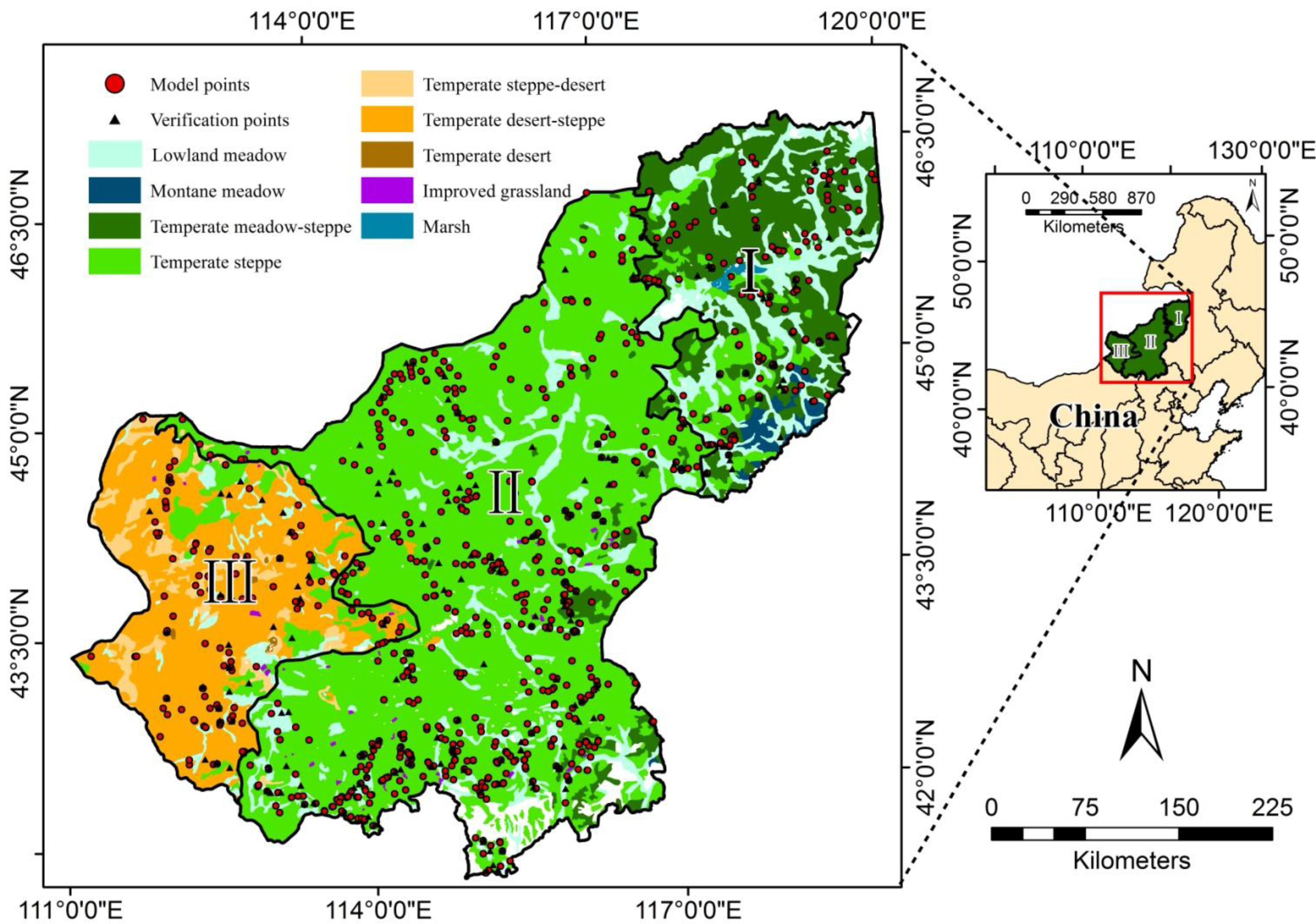
2.1. Study Area

Xilingol League is located in the central part of Inner Mongolia, between 41°35′ and 46°46′N and 111°09′ and 119°58′E. This area comprises natural pastures that are among the highest in quality in northern China. Xilingol is dominated by natural grasslands, and the total grassland area is 192,512 km2, representing 95.03% of the total area of the region. The study area is a typical temperate continental semi-arid climate. The mean annual temperature ranges from 1.3 °C to 4.8 °C, and the mean annual precipitation is approximately 150–400 mm, with a strong increasing gradient from the west to the east. The Xilingol grassland is primarily dominated by temperate meadow steppe, temperate steppe and temperate desert steppe (Figure 1).

2.2. Field data and Preprocessing

Field samples from this study area were obtained from the authors’ multi-year field survey data as well as the large-scale field campaign organized by the Grassland Monitoring and Supervision Center Ministry of Agriculture of China (GMSC), primarily in August from 2006 to 2012, when the green vegetation was at its peak. The sampling sites, each with an area of at least 1 km2, were chosen to represent typical vegetation communities. Each sampling site was homogeneous in terms of vegetation type and land type. For most sites, three plots were selected, with a distance greater than 250 m between plots. For herb or stunted brushwood plots (1 × 1 m), all plants were harvested to measure their fresh weight. For shrub plots (10 × 10 m), we sorted the plants into three groups according to their size (large, medium and small) and sampled the green parts along with the branches of the same year. The fresh weight of representative plant for a shrub clump was then multiplied by the number of shrub clumps to estimate the total fresh weight. For all sampling plots, the geographic coordinates, altitude, fresh weight, community coverage and plant height were recorded. The primary herb and shrub species included Leymus chinensis Trin., Stipa grandis P. Smirn., Achnatherum splendens Trin., Artemisia frigida Willd., Reaumuria soongorica Pall. and Lespedeza bicolor Turcz. Finally, we averaged the fresh weight of the three plots at the sampling site to produce the field sampling dataset.
The field sampling plots could respond to the growth conditions of the vegetation and represent the different grassland types to the greatest possible extent. In addition, we considered the topographic features of the plots and the ease of human access to the plots. Because the quality of the field sampling data could affect the accuracy of biomass estimation [26], we strictly examined and verified the sampling data by comparing the sampling values to the average biomass for different grassland types over several years. We eliminated abnormal samples that were not representative [16], and obtained a total of 1,134 biomass field samples (Figure 1).
The field sampling data were expressed in terms of wet weight. We converted the wet weights to air-dried weights using conversion coefficients for different grassland types [4,8,16,27] (Table 1) and further converted the air-dried weights to dry weights with 15% water content [28].

2.3. Remote Sensing Dataset and Preprocessing

MODIS products have been useful in regional- and global-scale grassland biomass estimation due to their wide viewing swath and high frequency of data acquisition [29]. MODIS reflectance data (MOD09Q1) were obtained from the US National Aeronautics and Space Administration. The data represented 8-day composites with 250-m spatial resolution corresponding to the time of field sampling. We obtained reflectance datasets (red and near-infrared bands) for 2006–2012 by applying reprojection, format conversion and mosaic using MODIS Reprojection Tools (MRT) software. The five VIs, which included the NDVI, DVI, EVI2, SAVI and MSAVI, were calculated using ENVI software with Equations (1)(5) [3034] as follows:
NDVI = ρ NIR ρ R ρ NIR + ρ R
DVI = ρ NIR ρ R
EVI 2 = 2.5 × ρ NIR ρ R ρ NIR + 2.4 ρ R + 1
SAVI = ( ρ NIR ρ R ) ( 1 + L ) ρ NIR + ρ R + L
MSAVI = 0.5 × [ 2 ρ NIR + 2 ( 2 ρ NIR + 1 ) 2 8 ( ρ NIR ρ R ) ]
where ρNIR and ρR correspond to the reflectance in the near-infrared and red wavelengths, respectively. L = 0.5 [33] and is the accommodation coefficient of the soil background.
Based on the sampling time and geographic coordinates of the field samples, we calculated the mean VI values within a circular area of each plot (in general, there were three to four pixels per mean value) using Geographic Information System (GIS) technology; subsequently, we established a database of VI versus biomass values within the corresponding period.

2.4. Development and Verification of Estimation Models

Because the Xilingol grassland includes nine different grassland types, it is difficult to characterize the precise biomass in the various grasslands using a single model [8,16]. Therefore, in view of the spatial distribution of grassland types and hydrothermal conditions, we divided the grassland of Xilingol into three regions to establish a different biomass estimation model for each region. These three regions were the meadow steppe region (I), the typical steppe region (II) and the desert steppe region (III).
Based on the correlation between the VIs and biomass in each region, we established regression models (linear function model, power function model, exponential function model and logarithm function model) in the three regions based on a random selection of 80% of the field data. We then calculated the root mean squared error (RMSE) and the mean relative estimation error (REE) to evaluate the precision of the estimation models using the reserved data (20% of the total samples). Finally, we selected a good model for each of the three regions based on the coefficient of determination (R2) and precision. All statistical analyses were performed using SPSS 17.0 and EXCEL 2010 software. The RMSE, REE and precision were calculated as follows Equations (6)(8):
RMSE = ( Y i Y i ) 2 N
REE = [ ( Y i Y i ) / Y i ] 2 N
Precision = ( 1 REE ) × 100 %
where Yi is the actual biomass of the field samples, Yi is the estimated grass yield and N is the sample size.

3. Results

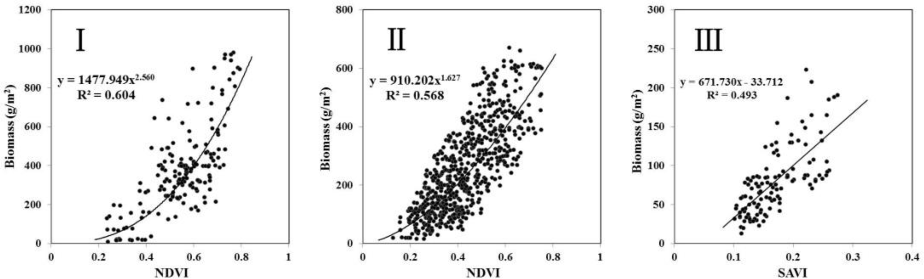
3.1. Relationship between Biomass and VIs

To understand the relationships between biomass and the VIs, we performed a correlation analysis between biomass and the five VIs in the three regions (Table 2). The results indicated that the biomass and the five VIs exhibited significant correlations (α < 0.01). Due to the variability of vegetation and hydrothermal conditions in the different grassland types, different VIs were applicable to different steppe regions. The correlation coefficients between biomass and VIs in the meadow steppe and typical steppe regions were higher than those in the desert steppe region. The correlation coefficients between biomass and NDVI in the meadow steppe and typical steppe regions were higher than those of the other VIs. The sequence of correlation coefficients in these two regions, ranked from high to low, was as follows: NDVI, SAVI, EVI2, MSAVI and DVI. However, in the desert steppe region, the correlation coefficients between biomass and EVI2, SAVI and MSAVI were higher than that between biomass and NDVI.

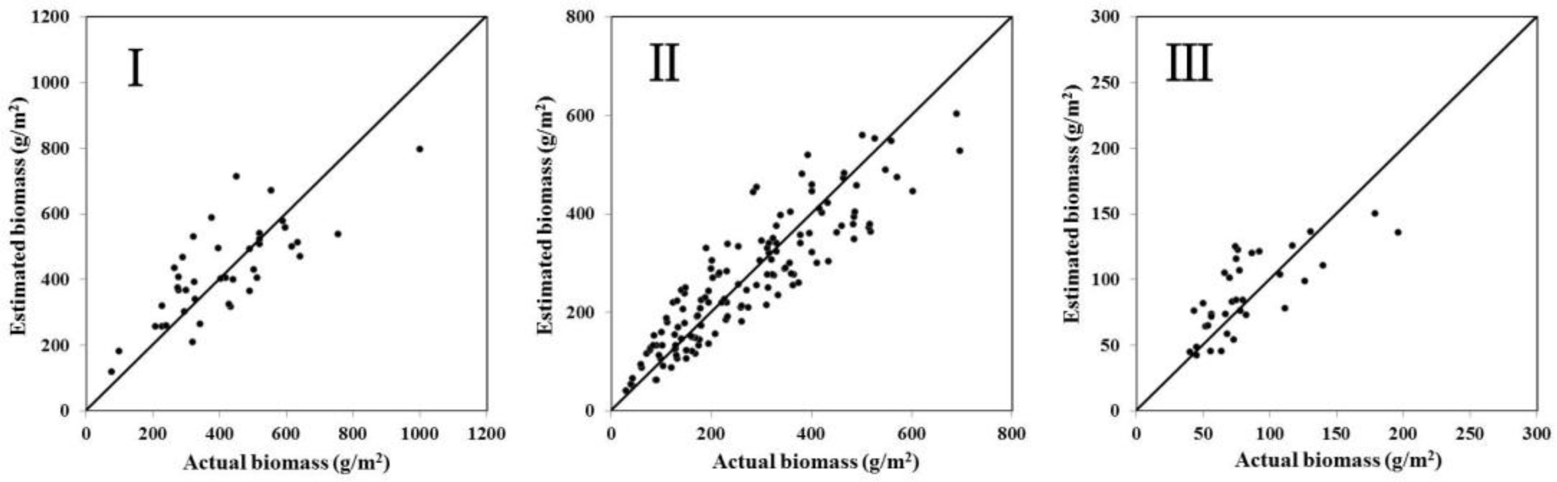
3.2. Development and Validation of Estimation Models

Among the established statistical models for biomass estimation (Table 3, Figures 2 and 3), the power function model relating NDVI to biomass showed the best performance for the meadow steppe region, with R2 = 0.604. The model precision was 73.6%, whereas the precision of the models using other VIs was less than 70%. Thus, we selected the power function model based on NDVI as the remote sensing monitoring model for the meadow steppe region. The statistical models for the typical steppe region were similar to the models for the meadow steppe region. We selected the power function model based on NDVI as the remote sensing monitoring model for the typical steppe region. The model precision for the relationship between biomass and NDVI was 73.9%. The correlation coefficient between biomass and VIs in the desert steppe region was lower than those in the other two regions, with R2 for the desert steppe ranging from 0.45 to 0.5. The linear functions with a precision greater than 73% for each VI were applied to the estimation of biomass in the desert steppe region. However, based on the R2 value, F value and precision, we ultimately selected the model given by a linear function of SAVI as the remote sensing monitoring model in the desert steppe region.

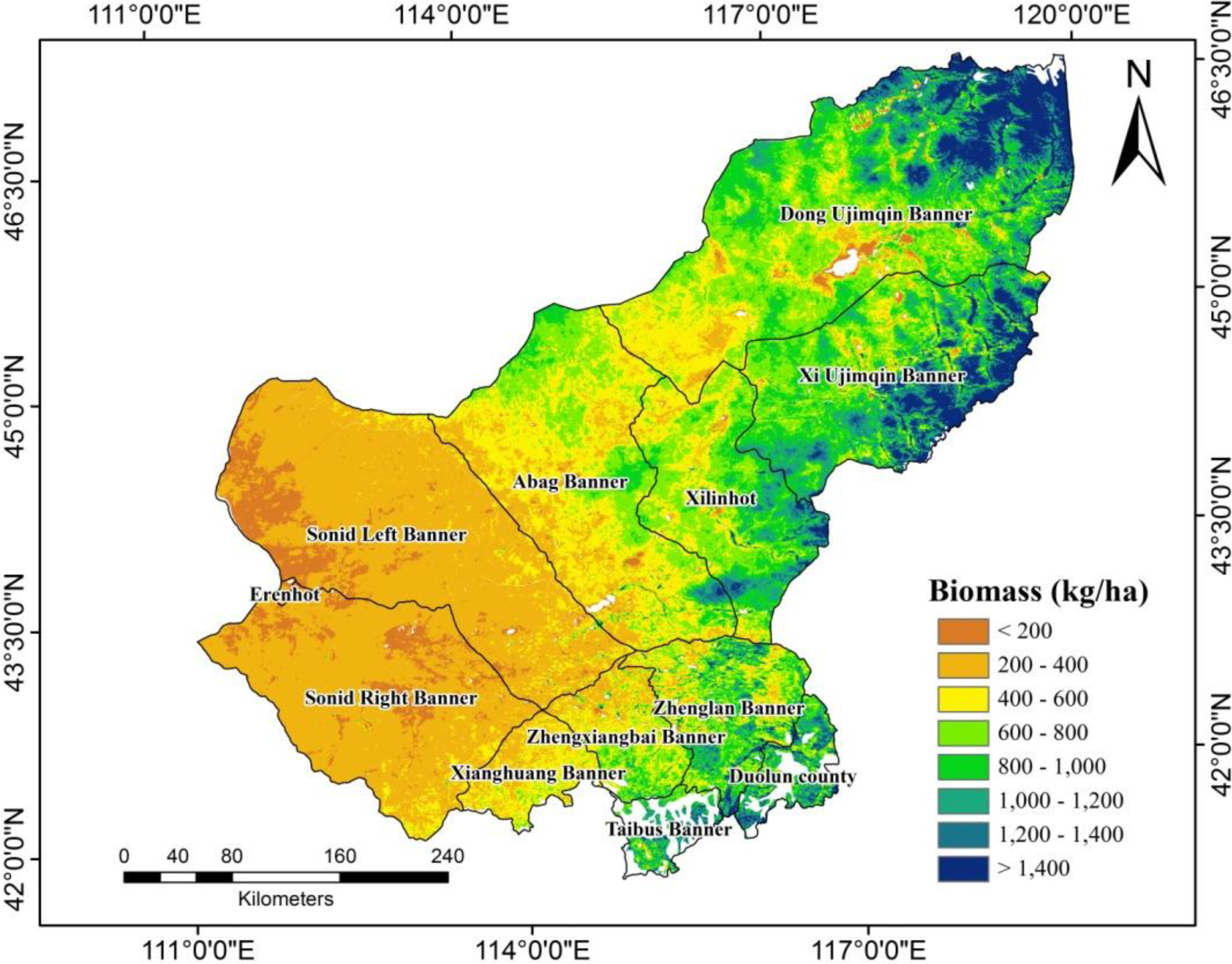
3.3. Spatial Distribution of Biomass in Xilingol

Based on the best estimation model for each of the three regions, we estimated the annual grassland biomass for each pixel using the VI at the peak period of the vegetation growing season from 2006 to 2012. We calculated the annual mean grassland biomass as the 7-year-average grassland biomass in Xilingol. As shown in Figure 4, the biomass in Xilingol exhibited substantial spatial heterogeneity and decreased from the eastern part to the western part of the study area. We then overlaid the 1:1,000,000 grassland type vector diagram on the biomass distribution for each grassland type.
According to the estimate of biomass in Xilingol from 2006 to 2012, the 7-year-average wet weight yield of biomass was 43.33 million tons, corresponding to biomass yield (dry weight) of approximately 11.86 million tons (Table 4). The average biomass was 604.5 kg/ha. The annual average yield of biomass was the highest at approximately 3.70 million tons in Dong Ujimqin Banner, representing 32.1% of the total biomass in Xilingol. The annual average yield of biomass in Xi Ujimqin Banner was 2.32 million tons. Because the biomass of those two Banners represented more than one-half of the total biomass, the two Banners had an important role in pasture management and the protection of grassland resources in Xilingol. The biomass was higher in southern Xilingol, including Duolun county and Taibus Banner. In addition, the highest densities of biomass in Xilingol, at more than 800 kg/ha, occurred primarily in the northeastern and southern Banners, which had better vegetation growth conditions and abundant grassland resources relative to the other areas.
According to the estimates of biomass for the different grassland types (Table 5), the temperate steppe area, which was the more extensive type representing 55.24% of the Xilingol grassland, had an annual biomass yield of 6.42 million tons. The values for the biomass yield of the temperate meadow-steppe and lowland meadow were the second highest of the various grassland types. The combined biomass yield of these three grassland types represented 90.7% of the total biomass yield in Xilingol. The biomass of the meadow steppe region was more than 1,000 kg/ha, whereas the highest biomass was associated with montane meadow at approximately 1,474.64 kg/ha. The biomass ranged from 500 to 1,000 kg/ha for the typical steppe region, and the biomass was estimated at less than 500 kg/ha in the desert steppe region, including temperate desert-steppe, temperate steppe-desert and temperate desert.

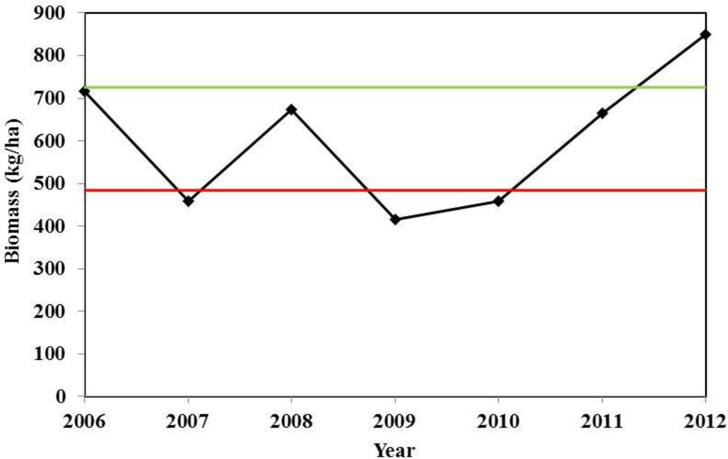
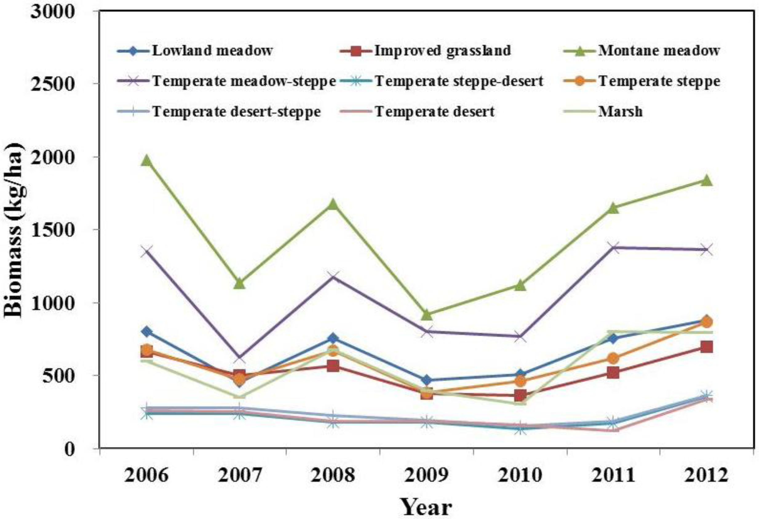
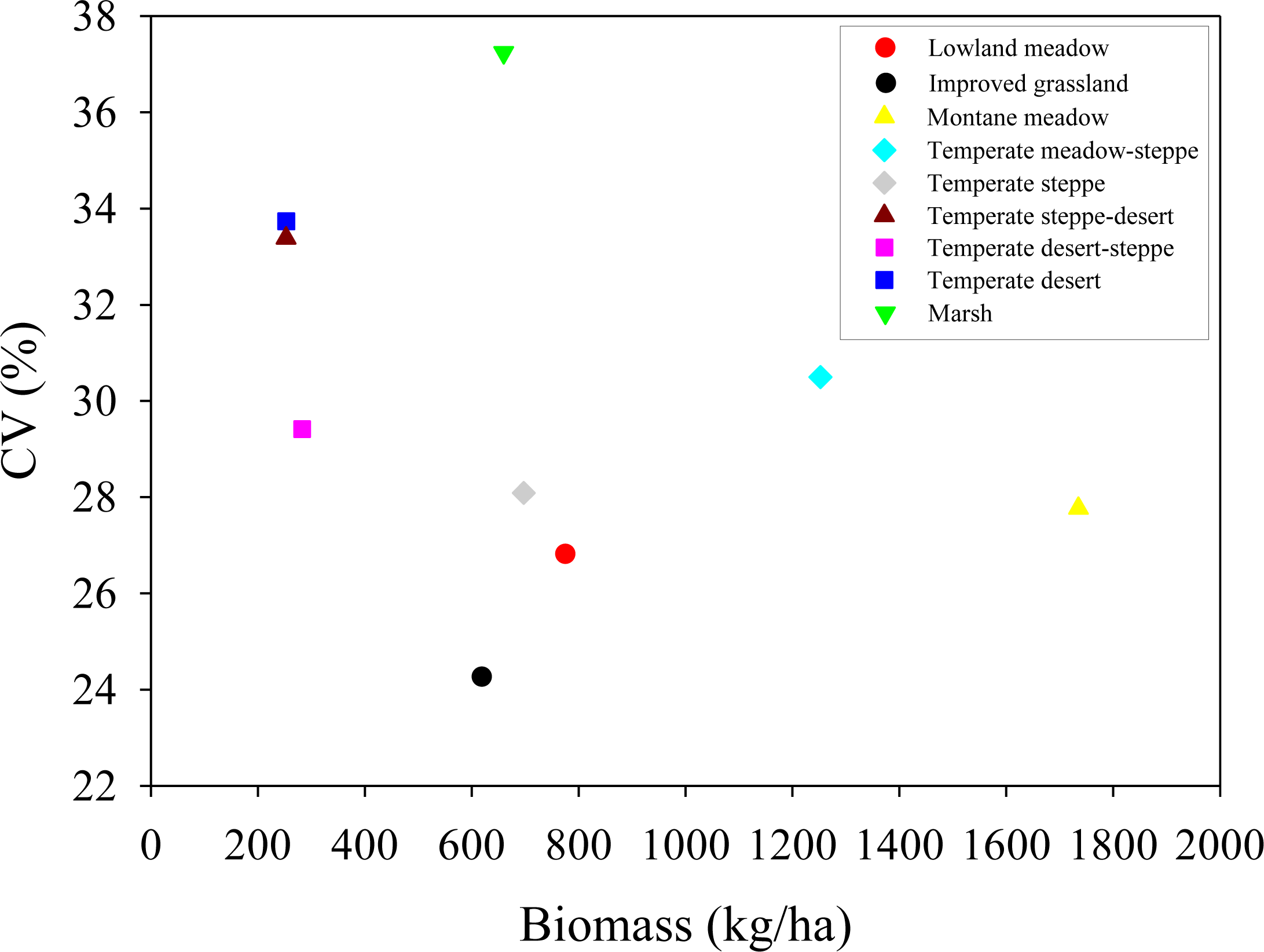
3.4. Interannual Variation of Biomass

Biomass in Xilingol exhibited obvious fluctuations (coefficient of variation (CV) = 26.95%), with the standard deviation (SD) of 162.94 kg/ha. These values were calculated from the annual variation in the entire average biomass of Xilingol. The lowest biomass occurred in 2009 at 415.38 kg/ha and was approximately 31% lower than the mean annual average biomass. The highest biomass was 849.26 kg/ha in 2012. This value was 40% higher than the mean annual average biomass and more than twice that of 2009. To analyze the interannual variations of biomass, we developed the categories Harvest Year, Lean Year and Common Year: a Harvest Year means that the biomass in the current year is more than 20% higher than the mean annual average biomass; a Lean Year means that the biomass in the current year is more than 20% lower than the mean annual average biomass; a Common Year falls between these values. As shown in Figure 5, the only Harvest Year occurred in 2012. The Lean Years were 2007, 2009 and 2010, for which the average biomass was 443.62 kg/ha. The Common Years were 2006, 2008 and 2011, for which the average biomass was 623.93 kg/ha.
The biomass of different grassland types appeared to fluctuate from 2006 to 2012 (Figure 6). The SD and CV values, which were calculated from annual variation in the entire average biomass of grassland types, responded to the fluctuations of biomass in different grassland types. The montane meadow showed the highest fluctuations of biomass, with an SD of 481.68 kg/ha. The highest biomass occurred in 2006 at 1,980.13 kg/ha, and the lowest biomass, at 919.03 kg/ha, occurred in 2009. The biomass in 2006 was 2.15 times that in 2009, with a CV of 27.8%. The fluctuations of biomass in temperate meadow-steppe were also high, with an SD of 382.0 kg/ha. The highest biomass for this vegetation type occurred in 2011, at 1,377.83 kg/ha, and the lowest biomass, at 624.74 kg/ha, occurred in 2007. The biomass in 2011 was 2.21 times that in 2007, and the CV was 30.5%. Additionally, the SD for lowland meadow was 207.85 kg/ha. The highest biomass for lowland meadow occurred in 2012 at 876.42 kg/ha, and the lowest biomass occurred in 2007, with a value of 455.14 kg/ha. The biomass in 2012 was 1.93 times that in 2007, and the CV was 26.8%.
The SD of temperate steppe was 195.84 kg/ha. The highest biomass occurred in 2012, at 868.92 kg/ha, and the lowest occurred in 2009 at 379.97 kg/ha. The biomass in 2012 was 2.29 times that in 2009, and the CV was 28.1%.
The magnitude of the fluctuations of biomass in temperate desert-steppe was lower than that in the other vegetation types, and the SD was only 83.08 kg/ha. The highest biomass of temperate desert-steppe occurred in 2012 at 361.76 kg/ha, and the lowest biomass, at 155.78 kg/ha, occurred in 2010. The biomass in 2012 was 2.3 times that in 2010, and the CV was 29.4%. The fluctuation pattern of temperate steppe-desert was the same as that of temperate desert-steppe, and the SD was 84.38 kg/ha. The highest and lowest biomass values were estimated in 2012 and 2010, respectively. The biomass in 2012 was 2.6 times that in 2010, and the CV was 33.4%. Because the areas of improved grassland, marsh and temperate desert represented less than 1% of the total grassland area, the fluctuations in these grassland types contributed minimally toward the total biomass yield of the study area.

4. Discussion

4.1. Model Development and Precision Validation

We selected five VIs (NDVI, DVI, EVI2, SAVI and MSAVI) for use in our study. NDVI is one of the most widely used VIs for estimating biomass. DVI is also commonly used. SAVI and MSAVI are suited to areas of low vegetation coverage due to their elimination or weakening of the interference from soil background information, whereas EVI2, based on EVI, uses only the red and near-infrared reflectance to obtain results similar to EVI. EVI2 can effectively weaken the noise caused by the soil or atmosphere. The correlation coefficient between NDVI and biomass in the meadow steppe and typical steppe regions was higher than that of the other VIs, and the power function model relating NDVI to biomass was superior to the other models. This model selection result was in agreement with other studies in Xilingol [13,35]. However, because the percent cover of soil was higher in areas with sparse vegetation, VI was more strongly affected by the interference from soil background information in the desert steppe region. The correlations between biomass and the three VIs (EVI2, SAVI and MSAVI) that better addressed soil interference in the desert steppe region were higher than those for the non-adjusted VIs, and the model weakened the interference from soil background information. Simultaneously, the precision of the linear model was higher than those of the other function models. This finding represented the critical difference between the estimation model for the desert steppe region and those for the meadow steppe and typical steppe regions.
At present, several models are available for estimating the biomass in one study area, although none have been confirmed as the optimal model, and a degree of uncertainty about the optimal model remains in each case. In this study, the models of estimated biomass have the following advantages: (1) In general, a high R2 or a low error level indicates a good fit in terms of model quality. In this study, we developed a biomass estimation model based on a collection of field sampling data and verified the precision of the models. The use of an extensive field sampling dataset established that the statistical models proved good reliability and accuracy. The estimated precision of the models was dependable, as we evaluated them using the reserved samples but not the modeling samples; (2) Because the biomass fluctuated each year, we developed the model using field sampling data for seven consecutive years. This approach was more stable than one based on field sampling data for a single year or several years; (3) Previous studies typically selected one month or several periods of 10-day VIs to estimate the biomass. This approach lacked temporal correspondence between the date of field data sampling and the date of remote sensing data acquisition. In our study, we ensured that the timing of field sampling and remote sensing data acquisition was consistent to the greatest possible extent. This approach enhanced the sensibility of the remote sensing data to reflect the vegetation biomass information; (4) Our findings suggested that biomass estimates on a large scale should be divided into different regions based on biophysical conditions. Within different regions, a suitable VI should be selected to identify the model that can best minimize the shortcomings of a single VI to estimate the biomass given heterogeneous vegetation.

4.2. Temporal and Spatial Variation of Biomass

Grassland types can affect the spatio-temporal patterns of biomass. Reflecting the location of the meadow steppe region in the eastern part of Xilingol and the gradual westward succession of typical steppe followed by desert steppe, the biomass decreased from east to west. Due to the abundant diversity of plant species and dense vegetation in the meadow steppe region, the biomass in this region was higher than in other grassland types. In addition, due to the large area of the meadow steppe region and differences in species composition, soil texture and hydrothermal conditions, the biomass of different meadow steppe types exhibited obvious spatial heterogeneity. In particular, the biomass of the montane meadow was the highest due to the favorable hydrothermal conditions and predominance of tall plant species. Additionally, the biomass of the typical steppe region was at an intermediate level, with typical xerophytic bunch grass. However, the desert steppe region is located in the temperate arid region, featuring perennial xerophytes and small bunch grasses, and presents a low, sparse appearance and seasonal uniformity. The biomass of the desert steppe region was lower than that of the meadow steppe and typical steppe regions [4].
Different patterns of interannual variations of biomass were also observed within the different grassland types. As shown in Figure 7, there was a negative but non-significant correlation between biomass and CV (R = −0.318, α = 0.405). With the increase of biomass in different grassland types, the CV decreased, whereas the stability of annual biomass increased. The range of biomass fluctuations for the meadow steppe types was greater than that for the other steppe types, although the CV for the meadow steppe types was lower than that for the other types. The source of this difference was the growth variations shown by the dominant plant species of the meadow steppe, Stipa baicalensis Roshev. and Leymus chinensis (Trin.) Tzvel. In years with abundant precipitation, these plant species grew well, and the biomass showed a marked increase. During drought years, plant growth was inhibited, and the biomass decreased substantially. However, because of the higher richness of plant species and higher biomass in the meadow steppe region, they inhibited the interannual variation of biomass [36]. In particular, the CVs of lowland meadow and montane meadow were low. These meadow steppe types were part of the intrazonal vegetation. These areas had better habitat and water conditions and experienced a weaker climate effect. Particularly in drought conditions, the biomass was higher and the interannual variation lower in these areas than in other steppe types [13].
Although the range of interannual fluctuation of biomass in the desert steppe region was lower than in the meadow steppe and temperate steppe regions, the CV was higher than in the other regions. The dominant plant species of the desert steppe region were Stipa klemenzii Roshev. and Caragana korshinskii Lam. Because of the lower absolute amount of biomass, relatively slight interannual fluctuations of the desert steppe ecosystem corresponded to a large range of fluctuation [37].

4.3. Differences between Biomass Estimates

Although several researchers have recently estimated the biomass of different grassland types in China using various methods, these estimates vary widely. For example, Ni [38] estimated carbon storage in 18 grasslands of China based on forage yield. We converted this carbon storage to biomass using a conversion factor for carbon (i.e., a carbon conversion factor of 0.45 was used to compare the estimates) [28]. The average biomass estimates for temperate desert-steppe, temperate steppe and temperate meadow-steppe were 455.6 kg/ha, 889.6 kg/ha and 1,464.7 kg/ha, respectively. Piao et al. [11] estimated the biomass of various grassland types in China between 1982 and 1999 based on time series data from NOAA/AVHRR-NDVI and field sampling data. The results indicated that the average biomass levels of temperate desert-steppe, temperate steppe and temperate meadow-steppe were 435.7 kg/ha, 915.2 kg/ha and 1,449.0 kg/ha, respectively. Our estimated average biomass values were lower than the corresponding values from these two studies. We used field sampling data from 2006 to 2012, whereas Ni and Piao used the first national grassland resource inventory from 1981 to 1988. Hence, the source of field data had a potentially significant impact on the estimation of biomass. Gao et al. [16] established a statistical model using field samples and MODIS-NDVI from 2005 to 2011 and estimated biomass in Inner Mongolia’s grassland. The average biomass values for temperate desert-steppe, temperate steppe and temperate meadow-steppe were 336.7 kg/ha, 600.4 kg/ha and 1,035.3 kg/ha, respectively. Our estimates of biomass in temperate steppe and temperate meadow-steppe were similar to those of Gao et al. [16], with a larger difference for temperate desert-steppe. In the present study, when plant species in temperate desert-steppe were sparse, the estimation model based on NDVI was influenced by soil background information. The precision of the estimation model using SAVI, which weakened the influence of the soil background information, was superior to that of the model using NDVI. In addition, variation among the research methods and the studied grassland regions also contributes to differences among estimates of biomass [27]. Additional uncertainties in the estimation of biomass are related to the characteristics of field samples, research methods and the study scale. Due to the different time frames for data collection and differences in the methods, even if the analysis is applied to the same data for one region, estimates of biomass can vary considerably based on several sources of variation and error. Additionally, the statistical models of the relationship between the field sampling data and VIs were expressed in terms of wet weight. When the biomass values were converted from wet to dry weight using the wet/dry conversion coefficients for grassland types, errors may have been introduced [16]. However, it was difficult to measure wet/dry ratios for each point in the entire coverage region based on ground observations. In the future, we should strengthen the measurement of the wet/dry weight ratios based on field sampling.

5. Conclusions

The estimation of biomass using a dataset of field samples and temporally corresponding remote sensing data can accurately reflect the temporal and spatial distribution characteristics of grassland vegetation and explore the interannual variation of biomass in different grassland types. Field sampling data provide the foundation needed to improve the precision of estimated biomass by remote sensing, and statistical models using several successive years of field sampling data can effectively enhance the stability of the estimates. The correlation coefficients between different VIs and biomass exhibit certain differences. Thus, one should select suitable VIs for different grassland type regions. The dominant plant species in different grassland types can affect the temporal and spatial distribution of biomass. Moreover, climatic factors such as precipitation and temperature affect the spatial distribution and interannual fluctuation of biomass [3941]. These considerations are subject to future discussion and analysis. Our study can serve as a reference for the effective protection and utilization of grassland resources as well as the scientific management of different regions and grassland types.

Acknowledgments

We are grateful for support from the National Natural Science Foundation of China (NSFC, 31372354), International Science & Technology Cooperation Program of China (2013DFR30760), the Agricultural Scientific Research Fund of Outstanding Talents and the Open Fund for the Key Laboratory of Agri-informatics, Ministry of Agriculture, China (2013010), and Grassland Monitoring and Supervision Center Ministry of Agriculture, China (326-6). We thank Grassland Monitoring and Supervision Center Ministry of Agriculture, China for providing the ground truth data.

Author Contributions

All authors contributed extensively to the work. Yunxiang Jin, Bin Xu designed and performed experiments. Bin Xu and Jianjun Qiu reviewed the manuscript and gave comments and suggestions to the manuscript. All authors performed the field survey. Yunxiang Jin, Xiuchun Yang, Tian Gao and Jinya Li validated the results with the field survey data. Qiong Wu, Hailong Ma, Fen Zhao and Haida Yu performed the satellite datasets preprocessing. Yunxiang Jin, Bin Xu and Qiong Wu wrote the manuscript. All authors participated in editing and revision of the paper.

Conflicts of Interest

The authors declare no conflict of interest.

References

  1. Adams, J.M.; Faure, H.; Faure-Denard, L.; McGlade, J.M.; Woodward, F.L. Increases in terrestrial carbon storage from the last glacial maximum to the present. Nature 1990, 348, 711–714. [Google Scholar]
  2. Scurlock, J.M.O.; Hall, D.O. The global carbon sink: A grassland perspective. Glob. Chang. Biol 1998, 4, 229–233. [Google Scholar]
  3. Peng, J.; Liu, Z.; Liu, Y.; Wu, J.; Han, Y. Trend analysis of vegetation dynamics in Qinghai—Tibet Plateau using Hurst Exponent. Ecol. Indic 2012, 14, 28–39. [Google Scholar]
  4. Department of Animal Husbandry and Veterinary, Rangeland Resources of China, 1st ed.; China Science and Technology Press: Beijing, China, 1996; pp. 188–207. (In Chinese)
  5. Scurlock, J.M.O.; Johnson, K.; Olson, R.J. Estimating net primary productivity from grassland biomass dynamics measurements. Glob. Chang. Biol 2002, 8, 736–753. [Google Scholar]
  6. Lu, D.S. The potential and challenge of remote sensing-based biomass estimation. Int. J. Remote Sens 2006, 27, 1297–1328. [Google Scholar]
  7. Flombaum, P.; Sala, O.E. A non-destructive and rapid method to estimate biomass and aboveground net primary production in arid environments. J. Arid Environ 2007, 69, 352–358. [Google Scholar]
  8. Xu, B.; Yang, X.C.; Tao, W.G.; Qin, Z.H.; Liu, H.Q.; Miao, J.M.; Bi, Y.Y. MODIS-based remote sensing monitoring of grass production in China. Int. J. Remote Sens 2008, 29, 5313–5327. [Google Scholar]
  9. Gaitán, J.J.; Bran, D.; Oliva, G.; Ciari, G.; Nakamatsu, V.; Salomone, J.; Ferrante, D.; Buono, G.; Massara, V.; Humano, G.; et al. Evaluating the performance of multiple remote sensing indices to predict the spatial variability of ecosystem structure and functioning in Patagonian steppes. Ecol. Indic 2013, 34, 181–191. [Google Scholar]
  10. Gao, Y.; Liu, X.; Min, C.; He, H.; Yu, G.; Liu, M.; Zhu, X.; Wang, Q. Estimation of the North-South Transect of eastern China forest biomass using remote sensing and forest inventory data. Int. J. Remote Sens 2013, 34, 5598–5610. [Google Scholar]
  11. Piao, S.L.; Fang, J.Y.; Zhou, L.M.; Tan, K.; Tao, S. Changes in biomass carbon stocks in China’s grasslands between 1982 and 1999. Glob. Biogeochem. Cycles 2007, 21. [Google Scholar] [CrossRef]
  12. Butterfield, H.S.; Malmström, C.M. The effects of phenology on indirect measures of aboveground biomass in annual grasses. Int. J. Remote Sens 2009, 30, 3133–3146. [Google Scholar]
  13. Jin, Y.X.; Xu, B.; Yang, X.C.; Li, J.Y.; Wang, D.L.; Ma, H.L. Remote sensing dynamic estimation of grass production in Xilingol, Inner Mongolia. Sci. Sin. Vitae 2011, 41, 1185–1195. [Google Scholar]
  14. Leisher, C.; Hess, S.; Boucher, T.M.; van Beukering, P.; Sanjayan, M. Measuring the impacts of community-based grasslands management in Mongolia’s Gobi. PLoS One 2012, 7. [Google Scholar] [CrossRef]
  15. Ouyang, W.; Hao, F.H.; Skidmore, A.K.; Groen, T.A.; Toxopeus, A.G.; Wang, T.J. Integration of multi-sensor data to assess grassland dynamics in a Yellow River sub-watershed. Ecol. Indic 2012, 18, 163–170. [Google Scholar]
  16. Gao, T.; Xu, B.; Yang, X.C.; Jin, Y.X.; Ma, H.L.; Li, J.Y.; Yu, H.D. Using MODIS time series data to estimate aboveground biomass and its spatio-temporal variation in Inner Mongolia’s grassland between 2001 and 2011. Int. J. Remote Sens 2013, 34, 7796–7810. [Google Scholar]
  17. Casady, G.; van Leeuwen, W.; Reed, B. Estimating winter annual biomass in the Sonoran and Mojave deserts with satellite- and ground-based observations. Remote Sens 2013, 5, 909–926. [Google Scholar]
  18. Lu, D.S. Aboveground biomass estimation using Landsat TM data in the Brazilian Amazon. Int. J. Remote Sens 2005, 26, 2509–2525. [Google Scholar]
  19. Mutanga, O.; Skidmore, A.K. Hyperspectral band depth analysis for a better estimation of grass biomass (Cenchrus ciliaris) measured under controlled laboratory conditions. Int. J. Appl. Earth Obs. Geoinf 2004, 5, 87–96. [Google Scholar]
  20. Anaya, J.A.; Chuvieco, E.; Palacios-Orueta, A. Aboveground biomass assessment in Colombia: A remote sensing approach. For. Ecol. Manag 2009, 257, 1237–1246. [Google Scholar]
  21. Ren, H.R.; Zhou, G.S.; Zhang, X.S. Estimation of green aboveground biomass of desert steppe in Inner Mongolia based on red-edge reflectance curve area method. Biosyst. Eng 2011, 109, 385–395. [Google Scholar]
  22. Yan, F.; Wu, B.; Wang, Y.J. Estimating aboveground biomass in Mu Us Sandy Land using Landsat spectral derived vegetation indices over the past 30 years. J. Arid Land 2013, 5, 521–530. [Google Scholar]
  23. Boschetti, M.; Bocchi, S.; Brivio, P.A. Assessment of pasture production in the Italian Alps using spectrometric and remote sensing information. Agric. Ecosyst. Environ 2007, 118, 267–272. [Google Scholar]
  24. Shinoda, M.; Gillies, J.A.; Mikami, M.; Shao, Y. Temperate grasslands as a dust source: Knowledge, uncertainties, and challenges. Aeolian Res 2011, 3, 271–293. [Google Scholar]
  25. Shiyomi, M.; Akiyama, T.; Wang, S.P.; Yiruhan; Ailikun; Hori, Y.; Chen, Z.Z.; Yasuda, T.; Kawamura, K.; Yamamura, Y. A grassland ecosystem model of the Xilingol steppe, Inner Mongolia, China. Ecol. Model 2011, 222, 2073–2083. [Google Scholar]
  26. Yang, X.C.; Xu, B.; Zhu, X.H.; Tao, W.G.; Liu, T.K. Models of grass production based on remote sensing monitoring in northern agro-grazing Ecotone. Geogr. Res 2007, 26, 213–221. [Google Scholar]
  27. Piao, S.L.; Fang, J.Y.; He, J.S.; Xiao, Y. Spatial distribution of grassland biomass in China. Acta Phytoecol. Sin 2004, 28, 491–498. [Google Scholar]
  28. Fang, J.Y.; Liu, G.H.; Xu, S.L. Carbon Pools in Terrestrial Ecosystems in China. In Emissions and Their Relevant Processes of Greenhouse Gases in China, 1st ed; Wang, G.C., Wen, Y.P., Eds.; China Environment Science Press: Beijing, China, 1996; pp. 109–128. (In Chinese) [Google Scholar]
  29. Muukkonen, P.; Heiskanen, J. Biomass estimation over a large area based on standwise forest inventory data and ASTER and MODIS satellite data: A possibility to verify carbon inventories. Remote Sens. Environ 2007, 107, 617–624. [Google Scholar]
  30. Rouse, J.W.; Haas, R.H.; Schell, J.A.; Deering, D.W. Monitoring Vegetation Systems in the Great Plains with ERTS. Proceedings of the Third Earth Resources Technology Satellite-1 Symposium, Washington, DC, USA, 10–14 December 1973; pp. 309–317.
  31. Tucker, C.J. Red and photographic infrared linear combinations for monitoring vegetation. Remote Sens. Environ 1979, 8, 127–150. [Google Scholar]
  32. Jiang, Z.; Huete, A.R.; Didan, K.; Miura, T. Development of a two-band enhanced vegetation index without a blue band. Remote Sens. Environ 2008, 112, 3833–3845. [Google Scholar]
  33. Huete, A.R. A soil adjusted vegetation index (SAVI). Remote Sens. Environ 1988, 25, 295–309. [Google Scholar]
  34. Qi, J.; Chehbouni, A.; Huete, A.R.; Kerr, Y.H.; Sorooshian, S. A modified soil adjusted vegetation index. Remote Sens. Environ 1994, 48, 119–126. [Google Scholar]
  35. Zhang, L.Y.; Zhang, J.X.; Sai, Y.J.Y.; Bao, H.X.; Shan, J.G.; Guo, Z.Z. Remote sensing monitoring model for grassland vegetation biomass monitoring in typical steppe: A case study from Xilingol. Pratacult. Sci 2008, 25, 31–36. [Google Scholar]
  36. Bai, Y.F.; Chen, Z.Z. Effects of long-term variability of plant species and functional groups on stability of a Leymus Chinensis community in the Xilin river basin, Inner Mongolia. Acta Phytoecol. Sin 2000, 24, 641–647. [Google Scholar]
  37. Hou, Y.Y.; Mao, L.X.; Li, C.S.; Qian, S. Spatiotemporal variation pattern of vegetation’s net primary productivity in China. Chin. J. Ecol 2008, 27, 1455–1460. [Google Scholar]
  38. Ni, J. Estimating net primary productivity of grasslands from field biomass measurements in temperate northern China. Plant Ecol 2004, 174, 217–234. [Google Scholar]
  39. Paruelo, J.M.; Lauenroth, W.K.; Burke, I.C.; Sala, O.E. Grassland precipitation-use efficiency varies across a resource gradient. Ecosystems 1999, 2, 64–68. [Google Scholar]
  40. Bai, Y.; Han, X.G.; Wu, J.G.; Chen, Z.Z.; Li, L.H. Ecosystem stability and compensatory effects in the Inner Mongolia grassland. Nature 2004, 431, 181–184. [Google Scholar]
  41. Hu, Z.; Fan, J.W.; Zhong, H.P.; Yu, G.R. Spatiotemporal dynamics of aboveground primary productivity along a precipitation gradient in Chinese temperate grassland. Sci. China Earth Sci 2007, 50, 754–764. [Google Scholar]
Figure 1. Spatial distribution of grassland types and sampling sites for three regions of Xilingol in Inner Mongolia, China. Region I is the meadow steppe region, Region II is the typical steppe region and Region III is the desert steppe region. The numbers of model points are 921 samples, and the numbers of verification points are 213 samples.
Remotesensing 06 01496f1
Figure 2. Relationship between VI and biomass: Region I, Region II and Region III. Region I and Region II selected the power function model based on NDVI; Region III selected the linear function model based on SAVI.
Remotesensing 06 01496f2
Figure 3. Relationship between the estimated and actual biomass values: Region I, Region II and Region III. The model precision for the relationship between the estimated biomass and the actual biomass was above 73%.
Remotesensing 06 01496f3
Figure 4. The 7-year-average grassland biomass between 2006 and 2012 in the Xilingol grassland.
Remotesensing 06 01496f4
Figure 5. Biomass variation in Xilingol grassland from 2006 to 2012. The green line is the Harvest Year threshold, and the red line is the Lean Year threshold. The black line is the interannual variation of biomass estimation.
Remotesensing 06 01496f5
Figure 6. The interannual variation of biomass in different grassland types.
Remotesensing 06 01496f6
Figure 7. Biomass-CV plot for different grassland types. Biomass was calculated as the 7-year-average grassland biomass in different grassland types. CV was calculated from the annual biomass of grassland types from 2006 to 2012.
Remotesensing 06 01496f7
Table 1. Conversion coefficients of grassland types.
Grassland TypesConversion CoefficientsGrassland TypesConversion Coefficients
Lowland meadow1/3.5Temperate steppe1/3.0
Improved grassland1/3.2Temperate desert-steppe1/2.7
Montane meadow1/3.5Temperate desert1/2.5
Temperate meadow-steppe1/3.2Marsh1/4.0
Temperate steppe-desert1/2.5
Table 2. Relationship between biomass and VIs in various regions. All relationships exhibit significant correlations. The correlation coefficients are calculated using all field samples (including model samples and verification samples) in different steppe regions.
BiomassNDVIDVIEVI2SAVIMSAVI
I Meadow steppe region (n = 214)0.7310.6640.7090.7110.708
II Typical steppe region (n = 766)0.7910.6410.7360.7430.728
III Desert steppe region (n = 154)0.6860.6930.7020.7020.702
Table 3. Statistical models of the estimated biomass and precision for the three regions.
Vegetation IndexModelR2F ValueRMSE (kg/ha)REEPrecision (%)
I Meadow steppe region (n = 173, test_n = 41)NDVIy = 1477.949x2.5600.604261.0961141.450.26473.6
DVIy = 507.373ln x + 1240.4080.464148.0161544.240.34665.4
EVI2y = 1711.819x − 182.1670.515181.9101376.940.31668.4
SAVIy = 1829.285x − 235.1480.518183.8891370.660.31368.7
MSAVIy = 1721.413x − 160.1140.515181.4231379.730.31868.2

II Typical steppe region (n = 629, test_n = 137)NDVIy = 910.202x1.6270.568825.644673.880.26173.9
DVIy = 2073.410x − 98.3970.387396.6411027.500.40359.7
EVI2y = 1344.033x − 110.7690.513611.698843.020.32167.9
SAVIy = 1403.755x − 140.0480.523687.838826.640.32567.5
MSAVIy = 1379.324x − 104.2730.502631.358862.300.33166.9

III Desert steppe region (n = 119, test_n = 35)NDVIy = 486.989x − 27.7190.484109.625281.910.26773.3
DVIy = 978.067x − 33.2730.475105.913255.290.26673.4
EVI2y = 677.344x − 28.4930.491113.082256.680.26074.0
SAVIy = 671.730x − 33.7120.493113.708258.960.26173.9
MSAVIy = 706.893x − 30.4120.490112.399255.450.26173.9
Note: n indicates the number of model samples; test_n indicates the number of verification samples; x indicates vegetation index; y indicates fresh biomass (g/m2).
Table 4. The annual biomass of different Banners.
Banner*Grassland Area (km2)Wet Weight of Biomass (t)Yield of Biomass (t)Biomass (kg/ha)
Abag Banner27,3255,085,4421,428,672522.84
Dong Ujimqin Banner43,86113,929,6483,701,216843.85
Duolun County2,9961,124,055300,3951,002.65
Erenhot1749,6183,028174.02
Sonid Left Banner34,6182,985,264895,988258.82
Sonid Right Banner25,1482,089,824614,094244.19
Xilinhot15,7134,175,0671,152,669733.58
Xi Ujimqin Banner23,5878,736,5532,323,326985.00
Xianghuang Banner4,885744,731208,519426.86
Zhenglan Banner10,1422,689,253743,844733.43
Zhengxiangbai Banner6,0841,170,427325,048534.27
Taibus Banner1,652590,210162,600984.26
Total196,18543,330,0941,1859,399604.50
Note:
*The Xilingol league includes twelve counties.
Table 5. The annual biomass of various grassland types.
Grassland TypesGrassland Area (km2)Wet Weight of Biomass (t)Yield of Biomass (t)Biomass (kg/ha)
Lowland meadow25,9557,041,8671,710,168658.90
Montane meadow1,593967,275234,9101,474.64
Temperate meadow-steppe24,6589,883,6462,625,3431,064.70
Temperate steppe108,3702,266,85516,422,757592.67
Temperate steppe-desert5,082321,088109,170214.82
Temperate desert-steppe29,5762,255,945710,205240.13
Temperate desert1408,8553,011215.04
Improved grassland47393,67824,883526.07
Marsh33889,18918,953560.73

