Article

Illumination and Contrast Balancing for Remote Sensing Images

1
Chongqing Institute of Green and Intelligent Technology, Chinese Academy of Sciences, Chongqing 400714, China
2
School of Remote Sensing and Information Engineering, Wuhan University, Wuhan 430079, China
3
State key Laboratory for Information Engineering in Surveying, Mapping and Remote Sensing, Wuhan University, Wuhan 430079, China
4
China Laboratory for High Performance Geo-computation, Shenzhen Institute of Advanced Technology, Chinese Academy of Sciences, Shenzhen 518055, China
*
Author to whom correspondence should be addressed.
Remote Sens. 2014, 6(2), 1102-1123; https://doi.org/10.3390/rs6021102
Submission received: 7 December 2013 / Revised: 17 January 2014 / Accepted: 17 January 2014 / Published: 28 January 2014

Abstract

:
Building a mathematical model of uneven illumination and contrast is difficult, even impossible. This paper presents a novel image balancing method for a satellite image. The method adjusts the mean and standard deviation of a neighborhood at each pixel and consists of three steps, namely, elimination of coarse light background, image balancing, and max-mean-min radiation correction. First, the light background is roughly eliminated in the frequency domain. Then, two balancing factors and linear transformation are used to adaptively adjust the local mean and standard deviation of each pixel. The balanced image is obtained by using a color preserving factor after max-mean-min radiation correction. Experimental results from visual and objective aspects based on images with varying unevenness of illumination and contrast indicate that the proposed method can eliminate uneven illumination and contrast more effectively than traditional image enhancement methods, and provide high quality images with better visual performance. In addition, the proposed method not only restores color information, but also retains image details.

1. Introduction

Satellite images are prone to the phenomenon of uneven illumination and contrast because of the atmospheric environment and climate condition while these images are being acquired. Satellite images that cover large areas, especially mosaic images, exhibit both uneven illumination and contrast distribution in some local areas [1,2]. This phenomenon has a negative influence on the further analysis and application of images since it will seriously affect the image quality and visual experience for human beings. Such images exhibit irregular and numerous uneven regional distributions of illumination and contrast which is difficult or even impossible to describe. Therefore, eliminating all unevenness, which is a process known as image balancing, is an important but difficult task, especially for mosaic images without any other auxiliary data.
After illumination and contrast balancing, an image should maintain the average intensity and overall hue of the original image as much as possible and have an even contrast in every part of the image. Various image enhancement methods have been proposed to achieve this objective. The histogram reflects the gray level distribution of an image. Thus, many histogram-based approaches [35], such as histogram equalization, brightness preserving bi-histogram equalization, minimum mean brightness error bi-histogram equalization (MMBEBHE), recursive mean separate histogram equalization (RMSHE), and light balancing [6,7] have been used to adjust the illumination and contrast of an image and these methods successfully enhance illumination and contrast while preserving input brightness to some extent. However, they might generate images that do not look as natural as the input images, which are unacceptable for remote sensing image products.
Homographic filter (HF) is also widely used to eliminate uneven illumination, compress dynamic range, and enhance contrast, thereby strengthening the high frequency and weakening the low frequency by separating incident and reflection components. However, image quality may degrade because the properties of additive and convolution noises in the frequency domain do not remain the same as those in the space domain. In addition, Fourier transform has a high computational cost, and selecting suitable transfer functions and parameters is difficult.
Recently, color constancy related to the human visual system and represented by retinex theory has become a hot topic in the image enhancement field [812]. Single-scale retinex [13], multi-scale retinex (MSR) [14], and MSR with color restoration (MSRCR) [15] are widely used. Unlike the HF method, the retinex approach needs to estimate the luminance image that is close to the actual scene. These methods successfully eliminate uneven illumination, thereby enhancing high-frequency information such as edges. However, they cannot effectively avoid uneven contrast.
Generally, the above methods can eliminate uneven illumination in an image. However, they are ineffective when processing images with both uneven illumination and contrast. Such images widely exist in practical application, especially in the image mosaic field.
Building a mathematical model is difficult or even impossible because of the complexity of uneven illumination and contrast. Considering that a satellite image covers a large area, illumination and contrast should change slowly, which produces a similar mean and standard deviation throughout an image. Hence, unevenness can be eliminated by adjusting the mean and standard deviation of a neighborhood at each pixel. In line with this principle, we proposed an image balancing method by using two balancing factors and linear transformation approach. Although the proposed method may change some physical properties of ground objects to some extent, the obtained results will show better visual performance. The proposed method consists of three steps: elimination of coarse light background, image balancing, and max-mean-min radiation correction.

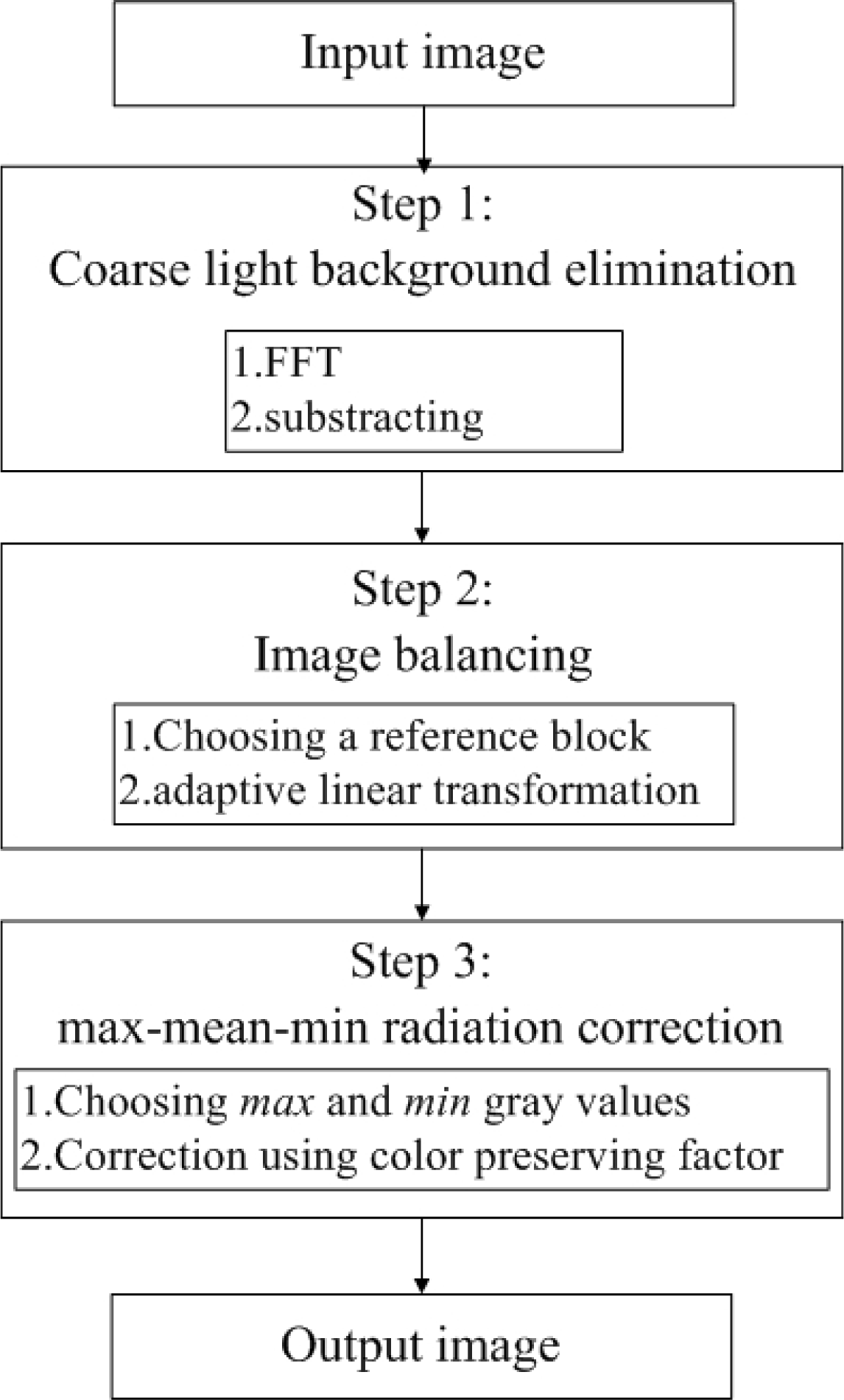
2. Proposed Image Balancing Method

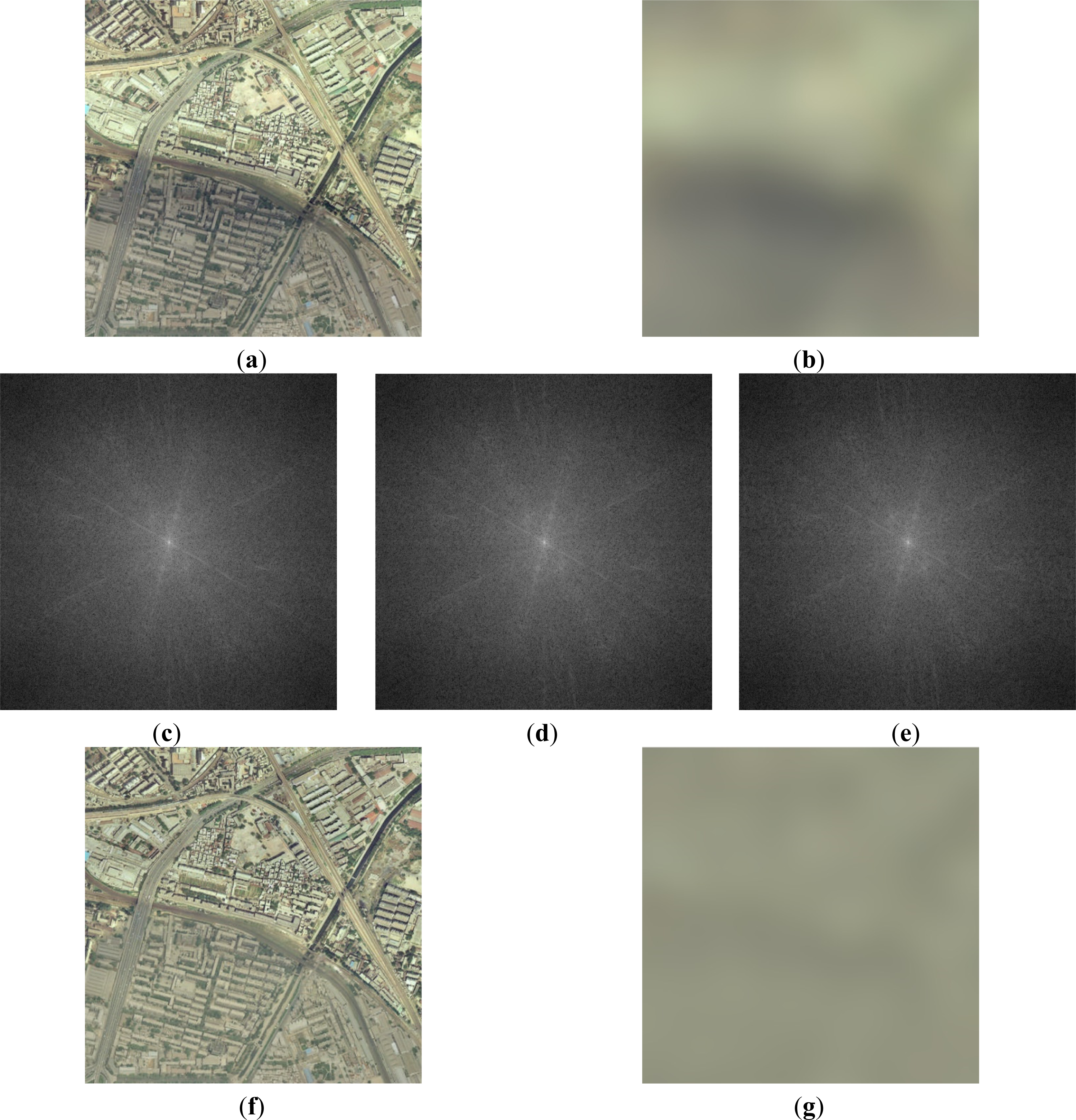
2.1. Coarse Light Background Elimination

The coarse light background means the overall brightness of an entire image. The main function of coarse light background elimination is to preliminarily balance this overall brightness, which is particularly important for an image that has contrasting colors. Radiation information of an image changes slowly in the space domain, whereas this information is related to low frequency in the frequency domain if fast Fourier transform (FFT) is applied to every image band
fft _ X = FFT ( X )
where X denotes any single band—either red, green, blue, or near-infrared—then the light background of X band can be estimated by applying the inverse FFT to the filtered result [16]:
B light = IFFT ( fft _ X × H )
where H is the low-pass filter in the frequency domain, such as Gaussian low-pass filter, and IFFT is the inverse FFT. Subtracting the light background from the input image in X band produces an image with coarse even illumination whereas maybe with uneven contrast
X ' ( x , y ) = X ( x , y ) B light ( x , y ) + X ( x , y ) ¯ + offset
where X ( x , y ) ¯ is the average value of X band, and offset is an constant that is often equal to zero. If the overall illumination of X band is too poor, offset can be set as a positive value to enhance X′. All the images used in this paper are obtained by Intergraph’s Z/I Imaging digital mapping camera (DMC) with a 0.3 m-resolution. The DMC has eight CCD sensors and is a dedicated camera for aerial photogrammetry with high resolution and high precision. It can obtain panchromatic and multispectral (blue, green, red, near-infrared bands) images simultaneously with different spatial resolution when working at different flight height. For better visual performance, these images are shown with different image sizes. Figure 1 shows the results of coarse light background elimination. The original image was a subset from an aerial mosaic image with a size of 512 × 512 pixels. Overall, the original image is properly illuminated. Therefore, the offset was set as zero.
The coarse light background (see Figure 1b) reflects the overall illumination of the image. The top part of Figure 1a is brighter than the bottom part, and the bottom part of image is smoother than the top part. Figure 1c,e are the frequency information of the original image. Figure 1f shows that the entire image is evenly illuminated because the light background is eliminated, whereas the bottom part still has a low contrast, which can also be seen from Figure 1g where the overall illumination is more even than that of Figure 1b.

2.2. Image Balancing

The second image balancing step needs a reference image with proper and even illumination and contrast. This image can be extracted from the original image manually or automatically after the first step has been performed. In the automatic approach, the whole image is evenly divided into many image blocks, and the block with the highest definition is chosen as the reference image. In this paper, the number of blocks is determined empirically, whereas it can be chosen according to image adaptively in the future work. The definition is expressed as
DE = 1 ( M 1 ) ( N 1 ) x = 1 M 1 y = 1 N 1 Δ x 2 + Δ y 2 2
where
Δ x = X block ( x + 1 , y ) X block ( x , y )
Δ y = X block ( x , y + 1 ) X block ( x , y )
M and N are the width and height, respectively, of image block Xblock (x, y), and x and y are the pixel coordinates.
According to the principle that every part of an image should have a similar mean and standard deviation, the following adaptive linear transformation is used to adjust the mean and standard deviation of a neighborhood at each pixel. Such neighborhood is an image area that surrounds the central pixel with a size = blk.
F ( x , y ) = α × X ( x , y ) + β
where a and β are two balancing factors that can be calculated adaptively
α = w s × Std ref / ( w s × Std nbr + ( 1 w s ) × Std ref )
β = w m × Mean ref + ( 1 w m α ) × mean nbr )
where Stdref and Stdnbr are the standard deviation of the reference image block and the neighborhood image block at the current pixel, respectively, and Meannbr and Meanref are the mean values of these two image blocks. ws and wm are the weights
w s = Std ref / ( Std ref + Std nbr )
w m = Mean ref / ( Mean ref + Mean nbr )
If the size of the neighborhood is set, the image balancing step can run adaptively. The size of the neighborhood will affect the image balancing result. A larger size will result in a smoother image, and vice versa, as shown in Figure 2.
Figure 2d–f is the subset image of Figure 2a–c in the red rectangle area, where Figure 2d is much sharper than Figure 2e,f, while Figure 2f is a little smoother than Figure 2e. This result can be seen from the definition values of Figure 2a–c in Table 1. The definition is calculated according to Equation (4). A higher definition value indicates a sharper image.
The larger size will result in more calculations. Numerous tests indicate that the sizes from 21 to 31 will ensure balance between image quality and calculation amount. Hence, in all the experiments, blk was set equal to 21. Compared with Figure 1c, the entire contrast of Figure 2a–c is more even. However, Figure 2a–c are still smooth images because the dynamic range of these images is too narrow, as indicated by the histograms shown in Figure 2g–i.

2.3. Max-Mean-Min Radiation Correction

After image balancing, some dark objects whose gray values should be close to zero show high values, whereas those bright objects tend to be dim. Hence, max-mean-min radiation correction is used to solve this problem.
Max-mean-min radiation correction uses the gray values of some of the darkest and brightest objects to adjust the other objects while maintaining the mean value of the image, and the pixel number of these darkest and brightest objects is small enough to have little influence on the whole image. Let M and N denote the height and width of the image, respectively. A scale parameter t is used to obtain a threshold T = tMN. The histogram of F(x,y) is defined as h(n), where n = 1, 2, …, 256. Then, the histogram values are accumulated from both left and right sides of the histogram, and the gray values that meet the following requirements are chosen as the max and min gray values:
{ i = 1 min h ( i ) T and i = 1 min + 1 h ( i ) > T j = 256 max h ( j ) T and j = 256 max 1 h ( j ) > T
The min and max are treated as gray values of the selected darkest and brightest objects. The temporary result that corresponds to F(x,y) is obtained as
Re ( x , y ) = { 0 , F ( x , y ) < min ( F ( x , y ) min ) meanv meanv min , min F ( x , y ) < meanv meanv + ( F ( x , y ) meanv ) 255 meanv max meanv , meanv F ( x , y ) < max 255 , F ( x , y ) max
where meanv is the mean value of F(x,y). Then a band of final image Re is
Re ( x , y ) = min { 255 , 255 × ( Re ( x , y ) 255 ) λ }
where λ is calculated by
λ = { ( maxv / 128 ) γ , maxv < 128 ( 128 / maxv ) γ , maxv 128
where γ is the color preserving factor with the value range [0, 1], and maxv is the maximum value of the histogram of F(x,y).
The scale parameter t is used to expand the dynamic range of the image. Figure 3a–c shows the results that were obtained with different t values, and Figure 3d shows the definition values of Figure 3a–c. A higher t value results in higher definition, which indicates that the image has higher contrast. This result was obtained because according to Equations (12) and (13), with the increase of t, an increasing number of pixel values were set as zero and 255, which increased the gradient and ultimately enhance the contrast. Various tests indicated that a t from 0.005–0.15 would obtain the proper results.
Equation (14) is used to further improve the color effect. Figure 4 shows the results with different γ values. A greater γ may result in more pixel values greater than 255, which means that the image exhibits excessive brightness (see Figure 4c), whereas a proper γ will produce a high-quality image. When γ = 0.05, Figure 4a is better than Figure 3a not only visually but also in objective aspects. The R, G, B band gradients of Figure 4a are 32.65, 33.46, and 33.09, respectively, and are much higher than those of Figure 3a. The histograms of the R, G, and B bands of Figure 4a are shown in Figure 4d–f, respectively. Compared with Figure 2g–i, the dynamic ranges are much wider, which indicates that the image quality is highly improved.
In Figure 4d–f, the frequencies of gray levels 0 and 255 are much greater than those of the other gray levels because that in Equation (13), the pixel gray values that are smaller than min value or greater than the max value are set as 0 and 255, respectively, to expand the dynamic range of the image. However, these pixels are too few to influence the whole image. Table 2 shows the number and ratio of these pixels before and after processing. Comparisons between the definition and color of Figures 1a and 4a indicate the effectiveness of the proposed image balancing method.
The overall flow chart of the proposed method is shown in Figure 5:
Figure 5. The flow chart of the proposed method.
Remotesensing 06 01102f5

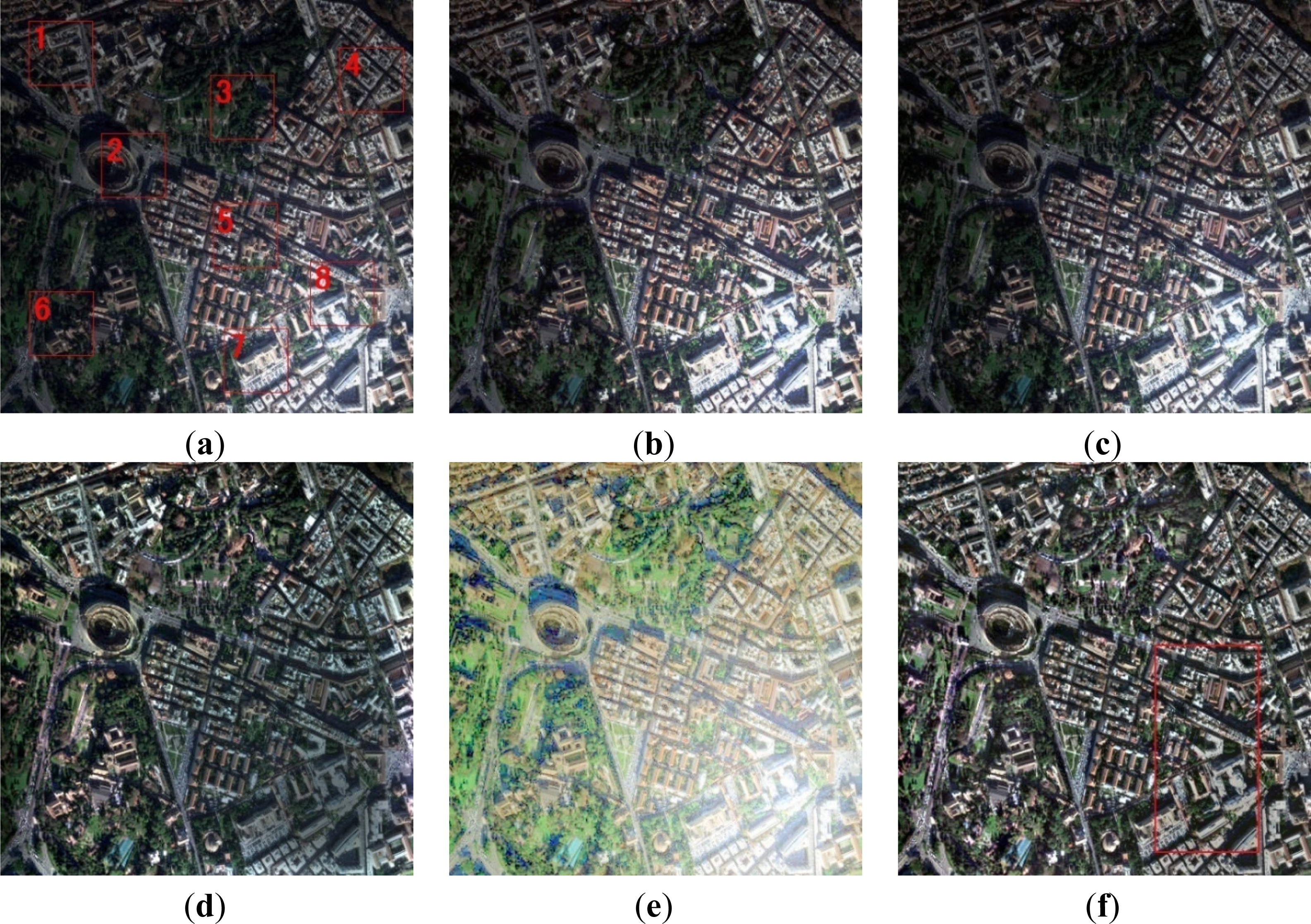
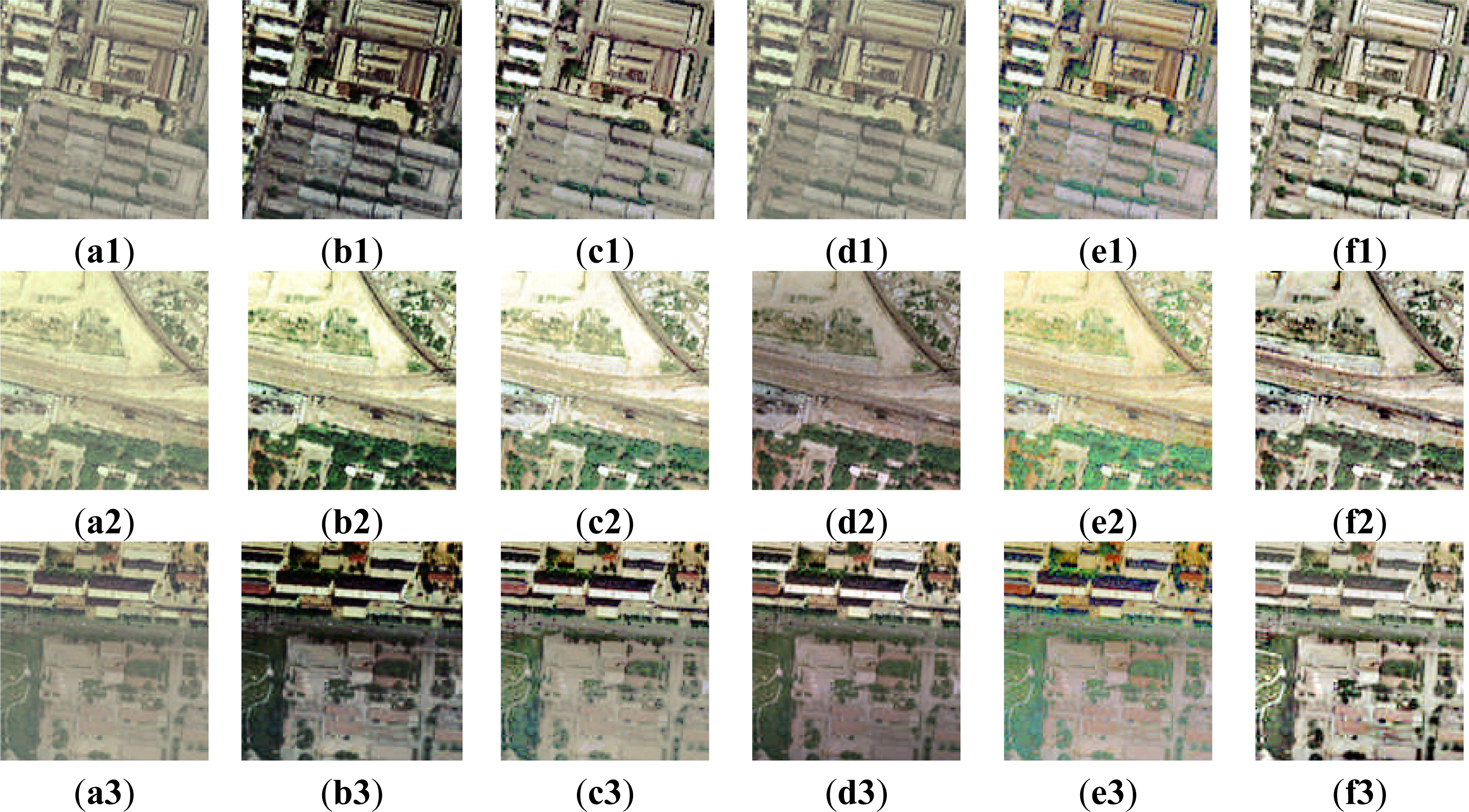
3. Experiments and Results

To evaluate the proposed image balancing method quantitatively, experiments on synthetic and real remote sensing images were carried out.

3.1. Experiments on Synthetic Image

Figure 4a was used as the standard image, which was then degraded horizontally, vertically, and centrally. In this experiment, only RMSHE and the proposed method were used to process the degraded images, and the results were compared with the standard image. The degraded and processed results are shown in Figure 6. For the proposed method, the offset values of Figure 6c,f,i were 50, 50, and 60, respectively, blk = 21, t = 0.005, γ = 0.05.
RMSHE only enhances the contrast of the bright areas. However, the degraded areas remain uneven and have low illumination and contrast. The proposed method effectively removes unevenness and produces images that have similar color and contrast as the standard image. The quantitative evaluations were carried out by using mean square error (MSE), peak signal-to-noise ratio (PSNR), and histogram flatness match (HFM).
The definition of MSE is:
MSE = 1 M × N i = 1 M i = 1 N ( X ( i , j ) X ( i , j ) ) 2
where (i, j) is the pixel coordinate, M and N represent the height and width of the image, respectively, and X and X′ denote the original and processed images, respectively. A smaller MSE value indicates that X and X′ are more similar.
The PSNR is expressed by using MSE:
PSNR = 10 × log ( 255 2 MSE )
The higher the PSNR value is, the more similar information the images X and X′ will have. HFM is calculated by using
HFM = 1 M × N i = 0 255 | H ' ( i ) H ( i ) |
where H and X′ are the histograms of the original and processed images, respectively. A lower HFM value indicates a better match between the processed image and the original image.
The quantitative values are presented in Table 3:
Table 3. Quantitative values of RMSHE and proposed method on synthetic image.
IdealHorizontalVerticalCentral

RMSHEProposedRMSHEProposedRMSHEProposed
MSER07,219.97278.387,787.54284.687,399.96251.34
G07,086.93271.637,654.24263.977,203.09221.47
B05,992.50209.886,369.60249.006,042.68176.41
Ave06,766.47253.307,270.46265.886,881.91216.41

PSNRR+∞9.545423.68449.216823.58729.438524.1281
G+∞9.626223.79099.291823.91529.555624.6776
B+∞10.354724.911010.089724.168710.318525.6654
Ave+∞9.842124.12889.532823.89049.770924.8237

HFMR01.51531.26801.39241.17601.41671.1303
G01.41091.20371.46280.89911.42491.2390
B01.54171.34971.47431.34371.47381.3733
Ave01.48931.27381.44321.13961.43851.2476
The proposed method undoubtedly outperforms RMSHE, which is consistent with the visual assessment.

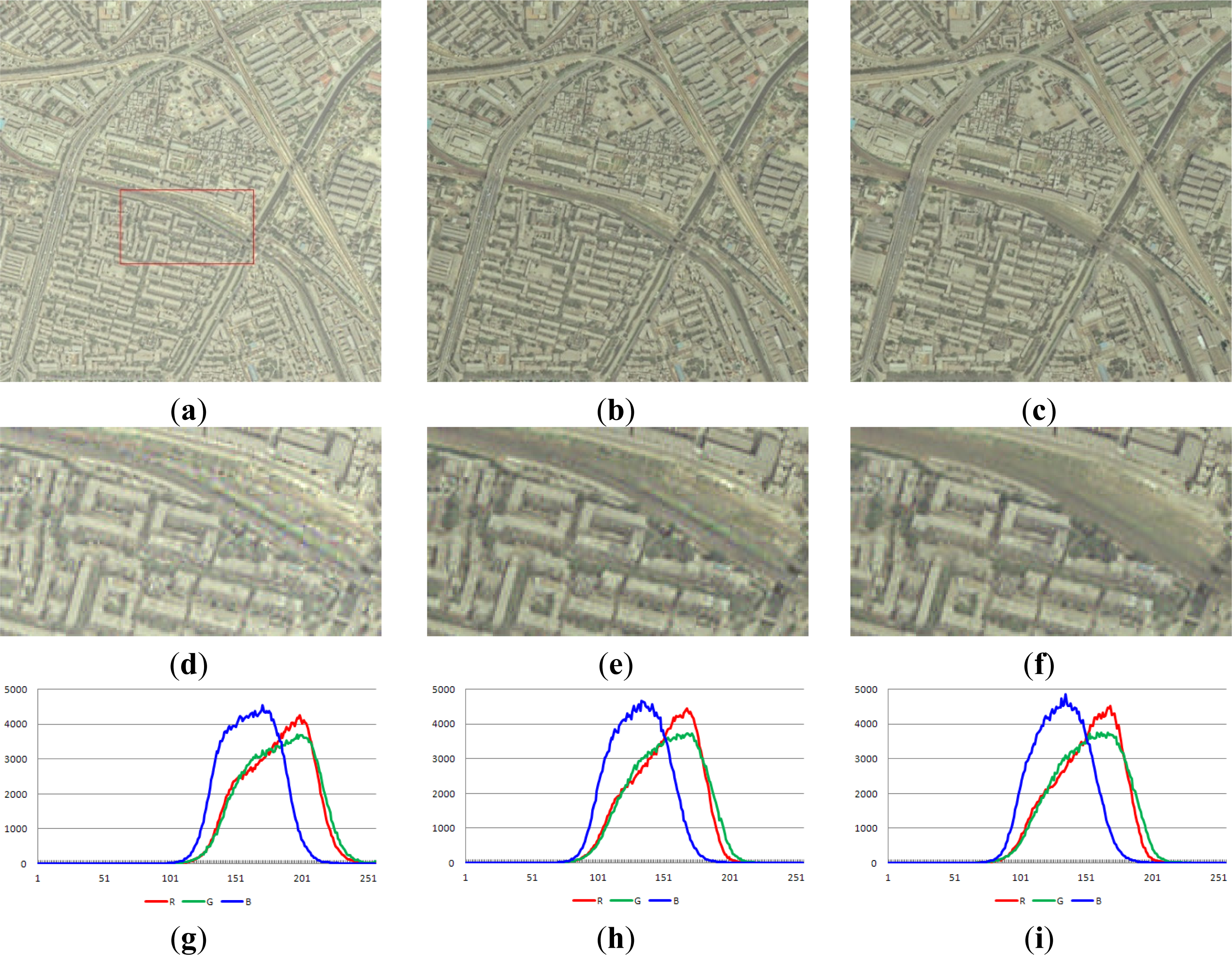
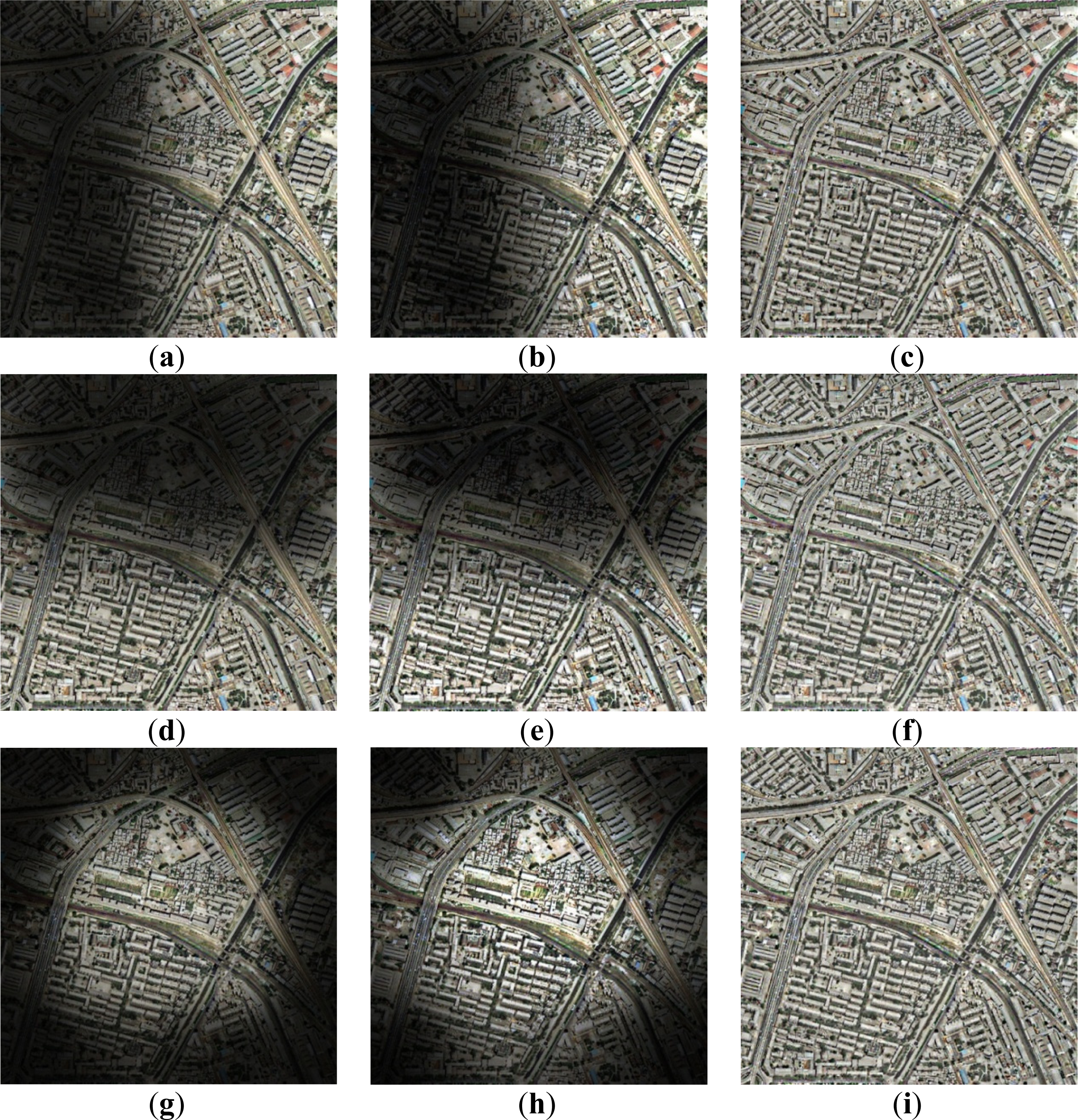
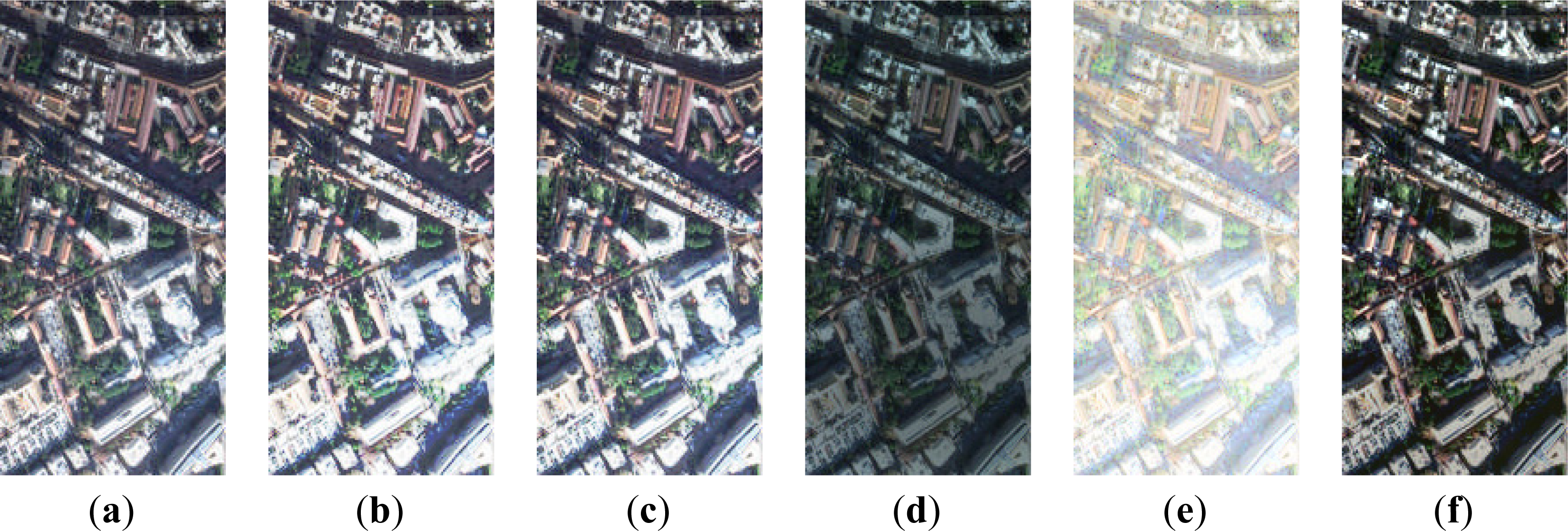
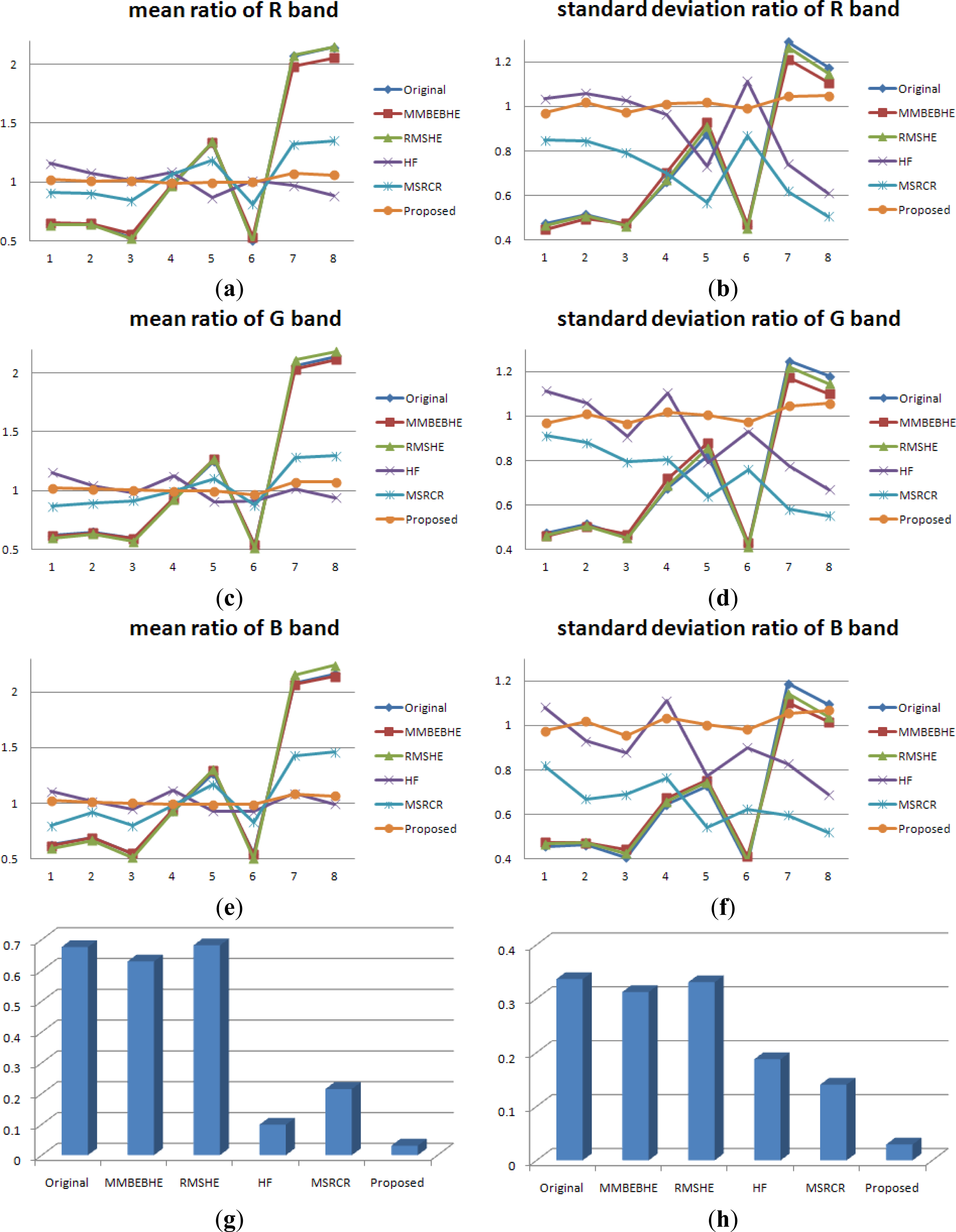
3.2. Experiments on Real Aerial Remote Sensing Images

Real aerial remote sensing images with different levels of uneven illumination and contrast were tested by using the proposed method, and our results were compared with those of HF, MMBEBHE, RMSHE, and MSRCR. Max-mean-min radiation correction was also used for HF and MSRCR methods. Figure 7 shows the results of the above methods, and Figure 8 shows the subset images of Figure 7. The red rectangle in Figure 7f was the boundary of subset images. The size of the original image was 512 × 512 pixels. The parameters of the proposed method were as follows: offset = 30, blk = 21, t = 0.005, γ = 0.05.
The brightness of the bottom-right corner of the original image is much higher than that of the other areas, whereas the contrast of the upper-left corner is much lower. The MMBEBHE, RMSHE, and MSRCR methods are unable to correct this phenomenon. The HF method can remove uneven illumination better than the other methods except for the proposed method. However, the contrast of the right side of Figure 7d is low. The proposed method provides the best result, as shown in the subset images in Figure 8.
Mean ratio and standard deviation ratio were used to evaluate the quality of images objectively. In Figure 7a, eight typical areas with a size of 80 × 80 pixels were selected in the red square and their mean and standard deviation values were calculated. For an image with proper illumination and contrast, the ratio of the mean value (MR) of a selected area to that of the whole image as well as the standard deviation ratio (SDR) should be close to one [17]. Hence, the performance of uneven illumination and contrast removal can be evaluated by checking the trends of mean and standard deviation ratio. Figure 9 shows the mean and standard deviation ratio of all bands of images in Figure 7. Since the standard deviation can reflect the dispersion degree of data, we also calculated the average standard deviation (ASD) of these two ratios as shown in Figure 9g,h. The smaller ASD will indicate the better visual performance.
The trends of mean and standard deviation ratios of MMBEBHE and RMSHE change intensely. The trend of MSRCR changes more slowly than that of MMBEBHE and RMSHE, and more quickly than the other methods. The mean and standard deviation ratios of the proposed method are both close to one in all bands, which indicates that the proposed method is the most effective. This can also be seen from the average standard deviation of these two ratios (MR and SDR) in Figure 9g,h, where the proposed method has the minimum ASD value; the ASD of MR of the proposed is only 4.41% of that of RMSHE, and this ratio of ASD of SDR is 8.63%.
Another image shown in Figure 10 was also a subset of a mosaic image with a size of 512 × 512 pixels. The top and bottom parts of the image were illuminated unevenly, and the bottom part was much smoother than the top part. Figure 10 shows the results of HF, MMBEBHE, RMSHE, MSRCR, and the proposed method. Max-mean-min radiation correction was also applied for HF and MSRCR methods. Figure 11 shows the subset images of Figure 10. The red rectangles in Figure 10f were three boundaries of subset images. The parameters of the proposed method were as follows: offset = 10, blk = 21, t = 0.005, γ = 0.05.
All methods can effectively enhance the contrast of the top part. However, with the exception of the proposed method, all the methods are unable to correct the bottom part. The differences between the proposed method and the other methods are evident based on Figures 10 and 11.
To assess the objective quality of these images, we evenly divided every image into five parts with five red squares shown in Figure 10a: upper left, bottom left, upper right, bottom right, and center. If an image has even illumination and contrast, the mean of these five parts and the standard deviation should be similar. Hence, the objective quality of results could be assessed by checking the similarity of the mean and standard deviation of these five parts. Figure 12 shows the mean and standard deviation values of the proposed method change gradually, whereas those of the other methods change significantly. The ASD of mean and standard deviation values were also calculated and shown in Figure 12c,d.
The above two experiments indicate that HF can eliminate uneven illumination better than MMBEBHE, RMSHE, and MSRCR. However, the HF results still show uneven contrast. Compared with the other methods, MMBEBHE and RMSHE produce images with higher contrast but have more uneven illumination. Therefore, uneven illumination and contrast still exists in images processed by using HF, MMBEBHE, RMSHE, and MSRCR; in contrast, the image results of the proposed method show high quality and good visual performance without any uneven illumination and contrast. The standard deviations of mean and standard deviation were shown in Figure 12c,d, where the minimum values are only 9.06% and 7.44% of the maximum values, respectively.

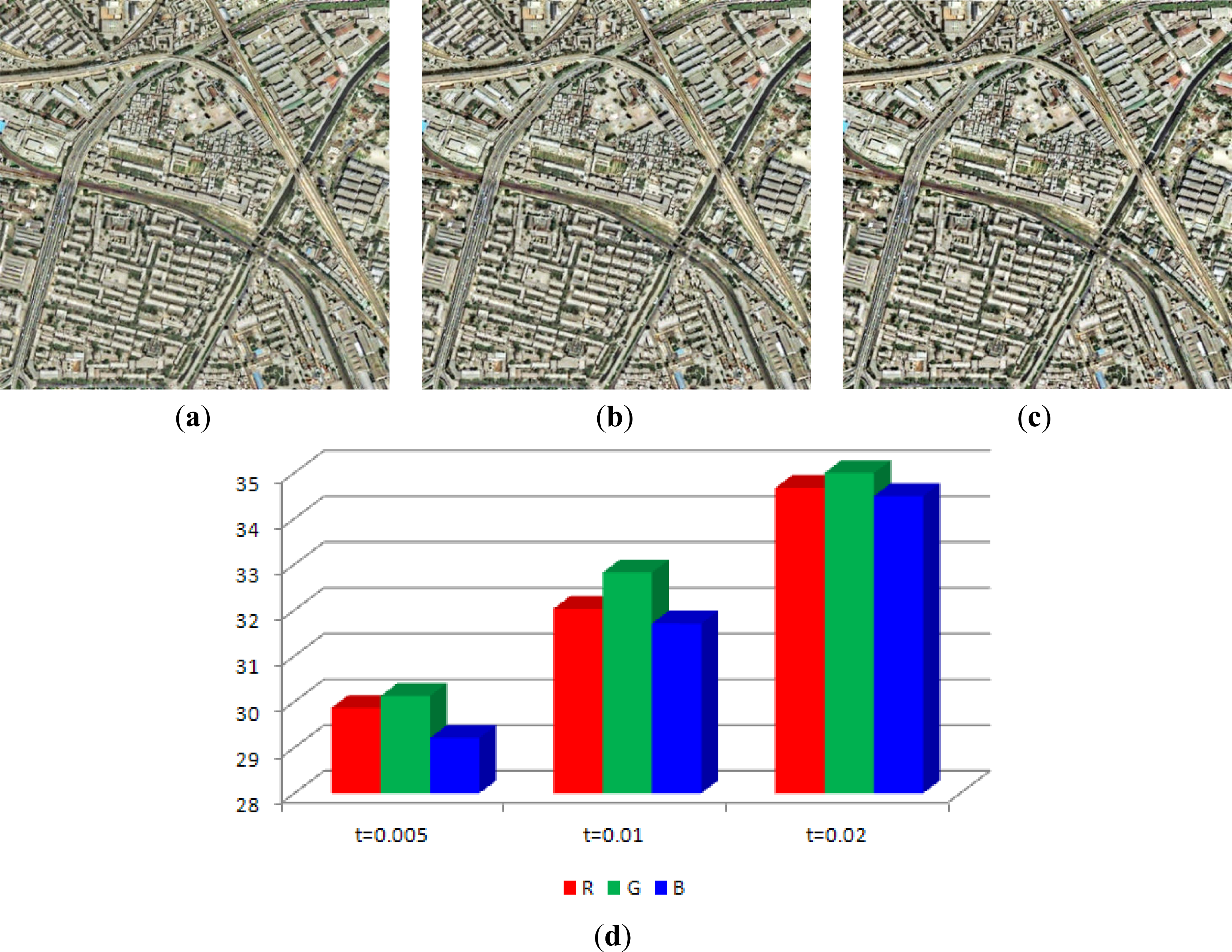
3.3. Efficiency Comparison

All the methods had been tested on the same platform (Thinkpad T430, Intel Core™ i5-3210M CPU, @2.50GHZ, 4.0G RAM, Windows 7, Matlab 7.0), and the CPU time of all methods were shown in Table 4. The unit of CPU time is second.
In the previous experiments, our method shows much better visual performance than the other methods. In Table 4, our proposed method needs much more time than the other methods due to the adaptive linear transformation in Section 2.2, since the mean and standard deviation of a neighborhood at each pixel should be adjusted. However, the adjusting computation of each pixel is independent, thus the adaptive linear transformation of the image balancing process is highly suitable for multi-core, parallel and GPU computing and the efficiency can be tremendously improved. Some other literatures have proved that this improvement can be up to scores or hundreds of times as high as the traditional CPU computing [18,19]. Hence, this issue is the main subject of our future work.

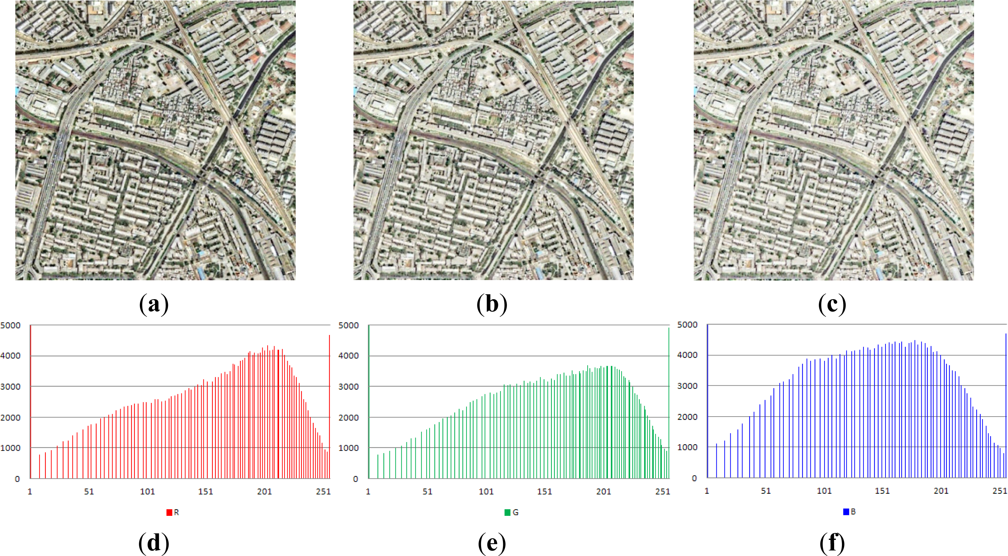
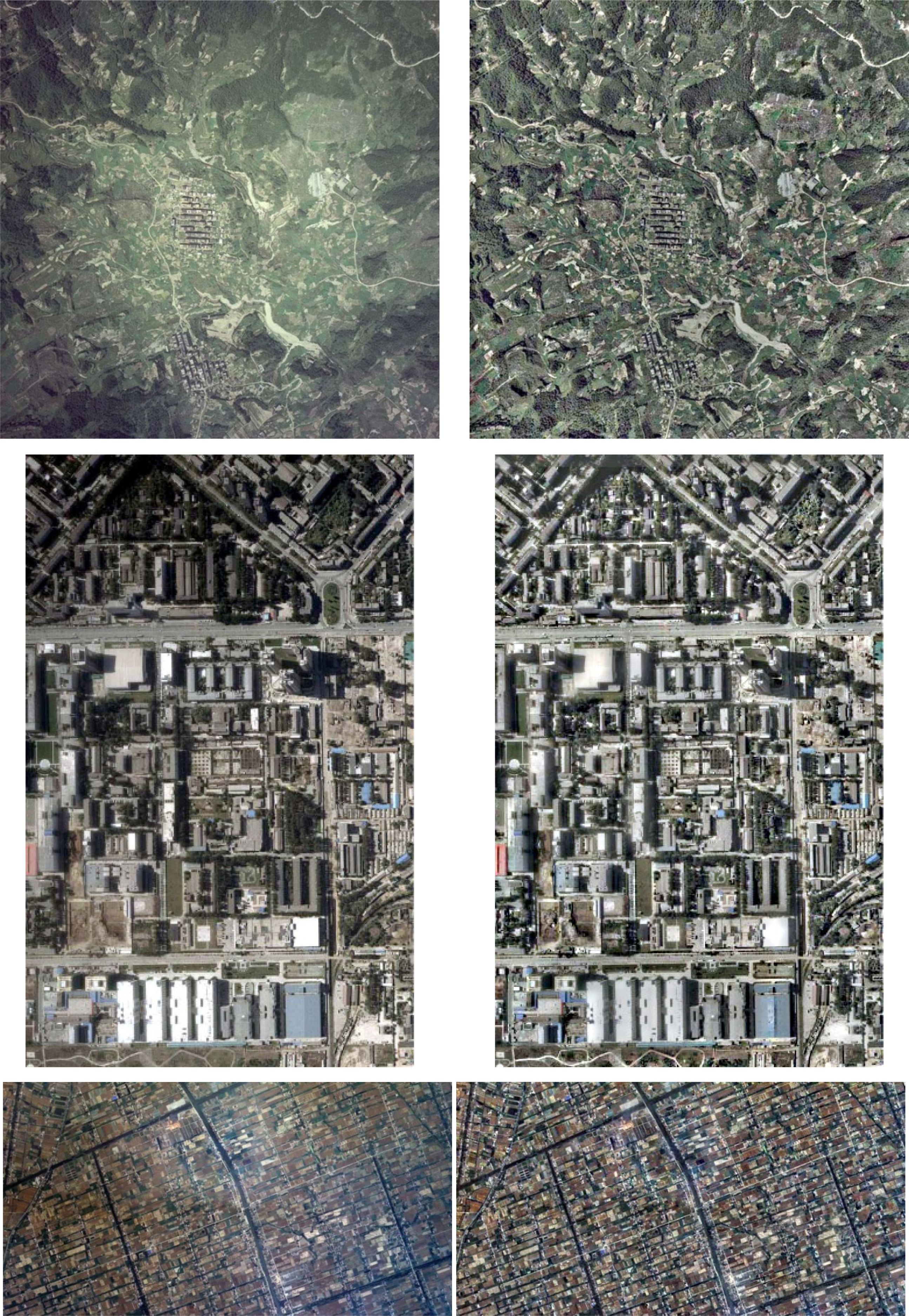
3.4. Experiments on More Aerial Remote Sensing Images

Some more images including a mosaic image and abnormal exposed images were tested and listed as follows in Figure 13 which also indicated the effectiveness of the proposed image balancing method.

4. Conclusions

Illumination and contrast balancing is an important but difficult task for remote sensing image applications, especially in the image mosaic field. Uneven illumination and contrast is complex, which is why building an accurate mathematic model is impossible. Existing image enhancing methods may not be able to efficiently address uneven illumination and contrast. Thus, this paper proposed an image balancing method without any other auxiliary data according to the principle that every part of a balanced image should have similar illumination and contrast. The proposed method consists of three steps: coarse light background elimination, image balancing, and max-mean-min radiation correction. Based on experimental results obtained by processing various remote sensing images with different levels of uneven illumination and contrast, the image balancing can be effectively achieved using the proposed method which outperforms existing image enhancement methods in visual performance and quantitative evaluation.
The main contributions of the proposed method include that this study proposed a feasible approach to estimate the coarse light background from an image so as to obtain an even overall brightness; according to an obvious principle, this study proposed an adaptive linear transformation to adjust the mean and standard deviation of a neighborhood at each pixel, so as to eliminate the uneven contrast; to solve the problem that some objects show untrue gray values, a max-mean-min radiation correction is proposed using no more than 2.5% of all pixel numbers to obtain a balanced image with proper illumination and contrast and fine visual performance. The image balancing effectiveness could be proven by the objective quality evaluations. For the first real aerial remote sensing image experiment, the average standard deviation of mean ration of the proposed method was only 4.41% of that of the method with maximum value, and the average standard deviation of standard deviation ratio was only 8.63%. In the second experiment, these two ratios were 9.06% and 7.44%, respectively. These results indicate that our method can provide images with the highest quality.
The proposed image balancing method is applicable to mosaic and other remote sensing imagery for visual enhancement of illumination and contrast. However, the main limitation is that it is more time-consuming than the existing methods. Therefore, the future work includes algorithm optimization using multi-core, parallel and GPU technologies, and ways to improve our method on other remote sensing images.

Acknowledgments

This work is jointly supported by the International Science and Technology Cooperation Program of China (No. 2010DFA92720-24); National Natural Science Foundation program (No. 41301403, No. 61172174, No. 40801165 and No. 10978003); Chongqing Basic and Advanced Research General Project (No. cstc2013jcyjA40010); Chongqing Major Programs for Science and Technology Development (No. CSTC2011GGC40008).

Author Contributions

Zhenfeng Shao is the corresponding author who theoretically proposed the whole method; Jun Liu implemented and improved the method and wrote the whole paper; Xing Wang, Min Chen and Shuguang Liu helped to implement the experiments and tested method on various remote sensing images; Xiran Zhou and Ping Liu involved in writing and revising the manuscript.

Conflicts of Interest

The authors declare no conflict of interest.

References

  1. Du, Y.; Cihlar, J.; Beaubien, J.; Latifovic, R. Radiometric normalization, compositing, and quality control for satellite high resolution image mosaics over large areas. IEEE Trans. Geosci. Remote Sens 2001, 39, 623–634. [Google Scholar]
  2. Zhu, S.L.; Zhang, Z.; Zhu, B.S.; Cao, W. Experimental comparison among five algorithms of brightness and contrast homogenization (In Chinese). J. Remote Sens 2011, 15, 111–116. [Google Scholar]
  3. Kim, M.; Chung, M.G. Recursively separated and weighted histogram equalization for brightness preservation and contrast enhancement. IEEE Trans. Consum. Elect 2008, 54, 1389–1397. [Google Scholar]
  4. Chen, S.D.; Ramli, A.R. Contrast enhancement using recursive mean-separate histogram equalization for scalable brightness preservation. IEEE Trans. Consum. Elect 2003, 49, 1301–1309. [Google Scholar]
  5. Menotti, D.; Najman, L.; Facon, J.; Araujo, A.A. Multi-histogram equalization methods for contrast enhancement and brightness preserving. IEEE Trans. Consum. Elect 2007, 53, 1186–1194. [Google Scholar]
  6. Hsia, S.C.; Chen, M.H.; Chen, Y.M. A cost-effective line-based light-balancing technique using adaptive processing. IEEE Trans. Image Process 2006, 15, 2719–2729. [Google Scholar]
  7. Hsia, S.C.; Tsai, P.S. Efficient light balancing techniques for text images in video presentation systems. IEEE Trans. Circuits Syst. Video Technol 2005, 15, 1026–1031. [Google Scholar]
  8. Jang, J.H.; Bae, Y.; Ra, J.B. Contrast-enhanced fusion of multisensor images using subband-decomposed multiscale retinex. IEEE Trans. Image Process 2012, 21, 3479–3490. [Google Scholar]
  9. Jang, J.H.; Kim, S.D.; Ra, J.B. Enhancement of optical remote sensing images by subband-decomposed multiscale retinex with hybrid intensity transfer function. IEEE Geosci. Remote Sens. Lett 2011, 8, 983–987. [Google Scholar]
  10. Jang, I.S.; Lee, T.H.; Kyung, W.J. Local contrast enhancement based on adaptive multiscale retinex using intensity distribution of input image. J. Imaging Sci. Technol 2011, 55, 040502. [Google Scholar]
  11. Rahman, Z.; Jobson, D.J.; Woodell, G.A. Investigating the relationship between image enhancement and image compression in the context of the multi-scale retinex. J. Vis. Commun. Image Represent 2011, 22, 237–250. [Google Scholar]
  12. Lee, S. An efficient content-based image enhancement in the compressed domain using retinex theory. IEEE. Trans. Circuits Syst. Video Technol 2007, 17, 199–213. [Google Scholar]
  13. Provenzi, E.; Carli, L.D.; Rizzi, A. Mathematical definition and analysis of the Retinex algorithm. J. Opt. Soc. Am. A 2005, 22, 2613–2621. [Google Scholar]
  14. Rahman, Z.; Jobson, D.D.; Woodell, G.A. Retinex processing for automatic image engancement. J. Electron. Imaging 2004, 13, 100–110. [Google Scholar]
  15. Liu, J.; Shao, Z.F.; Cheng, Q.M. Color constancy enhancement under poor illumination. Opt. Lett 2011, 36, 4821–4823. [Google Scholar]
  16. Li, D.R.; Wang, M.; Pan, J. Auto-dodging processing and its application for optical RS images. Geomat. Inf. Sci. Wuhan Univ 2006, 31, 753–756. [Google Scholar]
  17. Li, H.F.; Zhang, L.P.; Shen, H.F. A perceptually inspired variational method for the uneven intensity correction of remote sensing images. IEEE Trans. Geosci. Remote Sens 2012, 50, 3053–3065. [Google Scholar]
  18. Christophe, E.; Michel, J.; Inglada, J. Remote sensing processing: From multicore to GPU. IEEE J.-STARS 2011, 4, 643–652. [Google Scholar]
  19. Lee, C.A; Gasster, S.D.; Plaza, A. Chein-I chang, recent developments in high performance computing for remote sensing: A review. IEEE J.-STARS 2011, 4, 508–527. [Google Scholar]
Figure 1. Results of coarse light background elimination: (a) Original image; (b) Coarse light background of original image; (c) Fourier transform (FFT) result of R band of original image; (d) FFT result of G band of original image; (e) FFT result of G band of original image; (f) Elimination result; (g) Coarse light background of result image.
Remotesensing 06 01102f1
Figure 2. Effect of block size blk: (a) blk = 11, the red rectangle is the boundary of subset image; (b) blk = 21; (c) blk = 61; (d) subset of (a); (e) subset of (b); (f) subset of (c); (g) histogram of (a); (h) histogram of (b); (i) histogram of (c).
Remotesensing 06 01102f2
Figure 3. Effect of t: (a) t = 0.005; (b) t = 0.01; (c) t = 0.02; (d) definition of Figure 3a–c.
Remotesensing 06 01102f3
Figure 4. Effect of γ when t = 0.005: (a) γ = 0.05; (b) γ = 0.1; (c) γ = 0.15; (d) the histograms of the R band of Figure 4a; (e) the histograms of the G band of Figure 4a; (f) the histograms of the B band of Figure 4a.
Remotesensing 06 01102f4
Figure 6. Degraded and processed images: (a) Vertically degraded image; (b) Recursive mean separate histogram equalization (RMSHE) result of (a); (c) Proposed method result of (a); (d) Horizontally degraded image; (e) RMSHE result of (d); (f) Proposed method result of (d); (g) Centrally degraded image; (h) RMSHE result of (g); (i) Proposed method result of (g).
Remotesensing 06 01102f6
Figure 7. Image balancing results: (a) original image, eight typical areas with red squares are selected; (b) MMBEBHE; (c) RMSHE; (d) HF; (e) MSRCR; (f) proposed method with the boundary of subset images of Figure 8.
Remotesensing 06 01102f7
Figure 8. Subset of image balancing results in Figure 6: (a) Original image; (b) MMBEBHE; (c) RMSHE; (d) HF; (e) MSRCR; (f) Proposed method.
Remotesensing 06 01102f8
Figure 9. Mean and standard deviation ratio of results in Figure 6: (a) Mean ratio of R band; (b) Standard deviation of R band; (c) Mean ratio of G band; (d) Standard deviation of G band; (e) Mean ratio of B band; (f) Standard deviation of B band; (g) Average standard deviation of mean ratio of all bands; (h) Average standard deviation of standard deviation ratio of all bands.
Remotesensing 06 01102f9
Figure 10. Image balancing results: (a) original image which is divided into five parts shown in five red squares; (b) MMBEBHE; (c) RMSHE; (d) HF; (e) MSRCR; (f) proposed method with three boundaries of subset images of Figure 11.
Remotesensing 06 01102f10
Figure 11. Subset of image balancing results in Figure 6: (a1a3) original image; (b1b3) MMBEBHE; (c1c3) RMSHE; (d1d3) HF; (e1e3) MSRCR; (f1f3) proposed method.
Remotesensing 06 01102f11
Figure 12. Mean and standard deviation of five parts in all results: (a) Mean; (b) Standard deviation; (c) Standard deviation of mean; (d) Standard deviation of standard deviation.
Remotesensing 06 01102f12
Figure 13. Image balancing results: the (Left) are original images; the (Right) are image balancing results.
Remotesensing 06 01102f13aRemotesensing 06 01102f13bRemotesensing 06 01102f13c
Table 1. Definition values of Figure 2a–c.
RGB
blk = 1114.231815.058911.8794
blk = 2112.816913.631510.7306
blk = 6111.752612.53319.8586
Table 2. Number of pixels whose gray values equal 0 and 255.
RGB

025502550255
Number of pixels in the original image122311129040
Number of pixels in Figure 5a5,9146,1276,3094,6764,9304,702
Ratio2.26%2.25%2.41%1.35%1.88%1.78%
Table 4. CPU time of all the involved methods.
MMBEBHERMSHEHFMSRCRProposed
Figure 72.15320.34122.48963.485138.6113
Figure 102.21340.37012.52283.468938.5925

