Article

Land Surface Temperature Retrieval Using Airborne Hyperspectral Scanner Daytime Mid-Infrared Data

1
University of Chinese Academy of Sciences, Beijing 100049, China
2
Key Laboratory of Quantitative Remote Sensing Information Technology, Academy of Opto-Electronics, Chinese Academy of Sciences, Beijing 100094, China
3
College of Geography and Planning, Ludong University, Yantai 264025, China
4
College of Geomatics and Geoinformation, Guilin University of Technology, Guilin 541004, China
*
Authors to whom correspondence should be addressed.
Remote Sens. 2014, 6(12), 12667-12685; https://doi.org/10.3390/rs61212667
Submission received: 30 July 2014 / Revised: 15 October 2014 / Accepted: 1 December 2014 / Published: 16 December 2014
(This article belongs to the Special Issue Recent Advances in Thermal Infrared Remote Sensing)

Abstract

:
Land surface temperature (LST) retrieval is a key issue in infrared quantitative remote sensing. In this paper, a split window algorithm is proposed to estimate LST with daytime data in two mid-infrared channels (channel 66 (3.746~4.084 μm) and channel 68 (4.418~4.785 μm)) from Airborne Hyperspectral Scanner (AHS). The estimation is conducted after eliminating reflected direct solar radiance with the aid of water vapor content (WVC), the view zenith angle (VZA), and the solar zenith angle (SZA). The results demonstrate that the LST can be well estimated with a root mean square error (RMSE) less than 1.0 K. Furthermore, an error analysis for the proposed method is also performed in terms of the uncertainty of LSE and WVC, as well as the Noise Equivalent Difference Temperature (NEΔT). The results show that the LST errors caused by a LSE uncertainty of 0.01, a NEΔT of 0.33 K, and a WVC uncertainty of 10% are 0.4~2.8 K, 0.6 K, and 0.2 K, respectively. Finally, the proposed method is applied to the AHS data of 4 July 2008. The results show that the differences between the estimated and the ground measured LST for water, bare soil and vegetation areas are approximately 0.7 K, 0.9 K and 2.3K, respectively.

Graphical Abstract

1. Introduction

Land surface temperature (LST) is an important indicator for monitoring the changing of earth resources and one of the most critical parameters in the physical process of surface energy and water balance at local and global scales [1,2,3,4,5,6]. The knowledge of LST plays a valuable role in urban climate, evapotranspiration, vegetation assessment, heat flux estimation, hydrological cycle, and environment studies [7,8,9,10,11,12,13,14,15]. Therefore, it is necessary to find a reliable way to acquire LST in regional and global scales. With the development of remote sensing, infrared sensors, such as Moderate Resolution Imaging Spectroradiometer (MODIS), Advanced Very High Resolution Radiometer (AVHRR), and Spinning Enhanced Visible and Infrared Imager (SEVIRI), provide a valuable way for measuring LST over the entire globe.
To date, different methods have been proposed to retrieve LST from Thermal Infrared (TIR) remotely sensed data, such as the single channel algorithm and the split-window algorithm [16,17,18,19,20]. By comparison, the study on LST retrieval from Mid-Infrared (MIR) data is under-developed because the radiance measured during daytime in the MIR spectrum contains both the surface emitted thermal radiance and the reflected solar radiance, which are equal in magnitude [21,22]. Moreover, it is difficult to eliminate solar effects in the MIR spectrum during daytime because the separation of solar radiance from the total energy requires the accurate atmospheric information and the knowledge of the surface bidirectional reflectivity. However, the MIR data has its own advantages, such as higher detection sensitivity for high temperatures, higher atmospheric transmittance in the atmospheric window, and less sensitive to water vapor content (WVC) [22,23]. Therefore, Sun and Pinker proposed a split algorithm, with three TIR channels and one MIR channel, to retrieve LST from SEVIRI data [24]. The Visible Infrared Imaging Radiometer Suite (VIIRS) workgroup developed a dual split window day/night LST algorithm for 17 IGBP surface types by using two TIR bands (10.8 μm and 12 μm) and two MIR bands (3.75 μm and 4.005 μm), with a solar zenith angle cosine correction during the daytime [25]. Still, LST retrieval only from the Airborne Hyperspectral Scanner (AHS) daytime MIR data has not been studied. In this paper, a new method is proposed to retrieve LST from AHS daytime data in two MIR channels (channel 66: 3.746~4.084 μm and channel 68: 4.418~4.785 μm) after reducing/eliminating the effect of direct solar radiance.
Section 2 describes the theory associated with the LST retrieval and the procedures for AHS data simulation. The details of direct solar radiance estimation and LST retrieval, as well as the sensitivity analyses, are presented in Section 3 and Section 4, respectively. In Section 5, the proposed method is applied to AHS data, and the results are validated with in situ measurements. The conclusion is drawn in Section 6.

2. Methodology and Data Simulation

2.1. Basic Theory

Under local thermodynamic equilibrium during a clear-sky day, the radiative transfer equation (RTE) in the MIR region (3~5 μm) can be written as [15,26]:
B i ( T i ) = τ i [ ε i B i ( T s ) + ( 1 - ε i ) ( R a t m _ i + R a t m _ i s ) + ρ b i R i s ] + R a t m _ i + R a t m _ i s
where Bi is the Planck function. Bi(Ti) is the radiance measured at the top of the atmosphere (TOA) in channel i, and Ti is the brightness temperature. εi and Ts are the surface emissivity and surface temperature, respectively. τi is the transmittance of the atmosphere from the ground to the TOA along the viewing angle. R a t m _ i and R a t m _ i are the upward and downward atmospheric thermal radiances, respectively. R a t m _ i s and R a t m _ i s are the upward and downward solar diffusion radiances, respectively, which result from atmospheric scattering of the solar radiance. ρbi is the surface bidirectional reflectivity. R i s is solar radiance at ground level. In addition, R i s =   E i c o s ( θ s ) τ i ( θ s , φ s ) / π , where Ei is the solar irradiance at TOA, τ i ( θ s , φ s ) is the transmittance of the atmosphere from TOA to the ground along the solar angle, and θ s and φ s are the solar zenith and azimuth angle, respectively.
Equation (1) can be rewritten as follows:
B i ( T i ) = B i ( T i ) τ i ρ b i R i s = τ i [ ε i B i ( T s ) + ( 1 - ε i ) ( R a t m _ i + R a t m _ i s ) ] + R a t m _ i + R a t m _ i s
where B i ( T i ) is the radiance after extracting the reflected solar direct radiance, and T i is the equivalent brightness temperature.

2.2. Data

To develop the LST retrieval method, the at-sensor radiances should be simulated. For this purpose, the MODTRAN 4.0 radiative transfer code has been used to predict the radiances for the AHS MIR channels (CH66 and CH68) in terms of the channel filter functions [27]. In total, 705 atmospheric profiles, with the atmospheric bottom temperature (Ta) of 250~310 K and the WVC of 0.06~5.39 g/cm2, extracted from the TOVS Initial Guess Retrieval (TIGR) database [28,29], are used to analyse atmospheric effects. The attenuation of the surface radiance has been considered by adding the uniformly mixed gases (CO2, N2O, CO and CH4) and ozone, included in the standard atmospheres of the MODTRAN 4.0 code, to the water vapor taken from profiles in the TIGR radiosoundings [30]. To accomplish this, a previous classification of the surface temperature is made with the rule that the surface temperatures are from Ta − 5 K to Ta + 15 K with a step of 5 K. Furthermore, the VZAs are set to be 0°, 33.56°, 44.42°, 51.32°, 56.25°, and 60° (corresponding values of 1/cos(VZAs) are 1, 1.2, 1.4, 1.6, 1.8, and 2.0), respectively, so that 1/cos(VZAs) could be sampled with a step of 0.2. The SZAs are set as 0°, 25.84°, 36.87°, 45.57°, 53.13°, and 60° (cos(SZAs) are 1, 0.9, 0.8, 0.7, 0.6, and 0.5), respectively, so that the cos(SZAs) could be sampled with a step of 0.1. Also, 70 different emissivities obtained from the Johns Hopkins University (JHU) Spectral library (soils, vegetation, and water, etc.) are considered. Once the simulations are made, TOA radiance could be determined according to Equation (1). In total, for the TIGR database and the JHU Spectral library, 8,883,000 different situations are simulated for retrieval.

2.3. LST Retrieval Method from Two AHS MIR Channels

The daytime MIR radiance contains not only the radiance emitted by the land surface and atmosphere but also the solar radiance reflected by the land surface and scatted by the atmosphere. To retrieve LST from MIR data, the direct solar radiance should be estimated first to eliminate the effect of solar radiance, and then a split window method should be developed to estimate the LST using the radiance ( B i ( T i ) ) after extracting the reflected solar direct radiance.

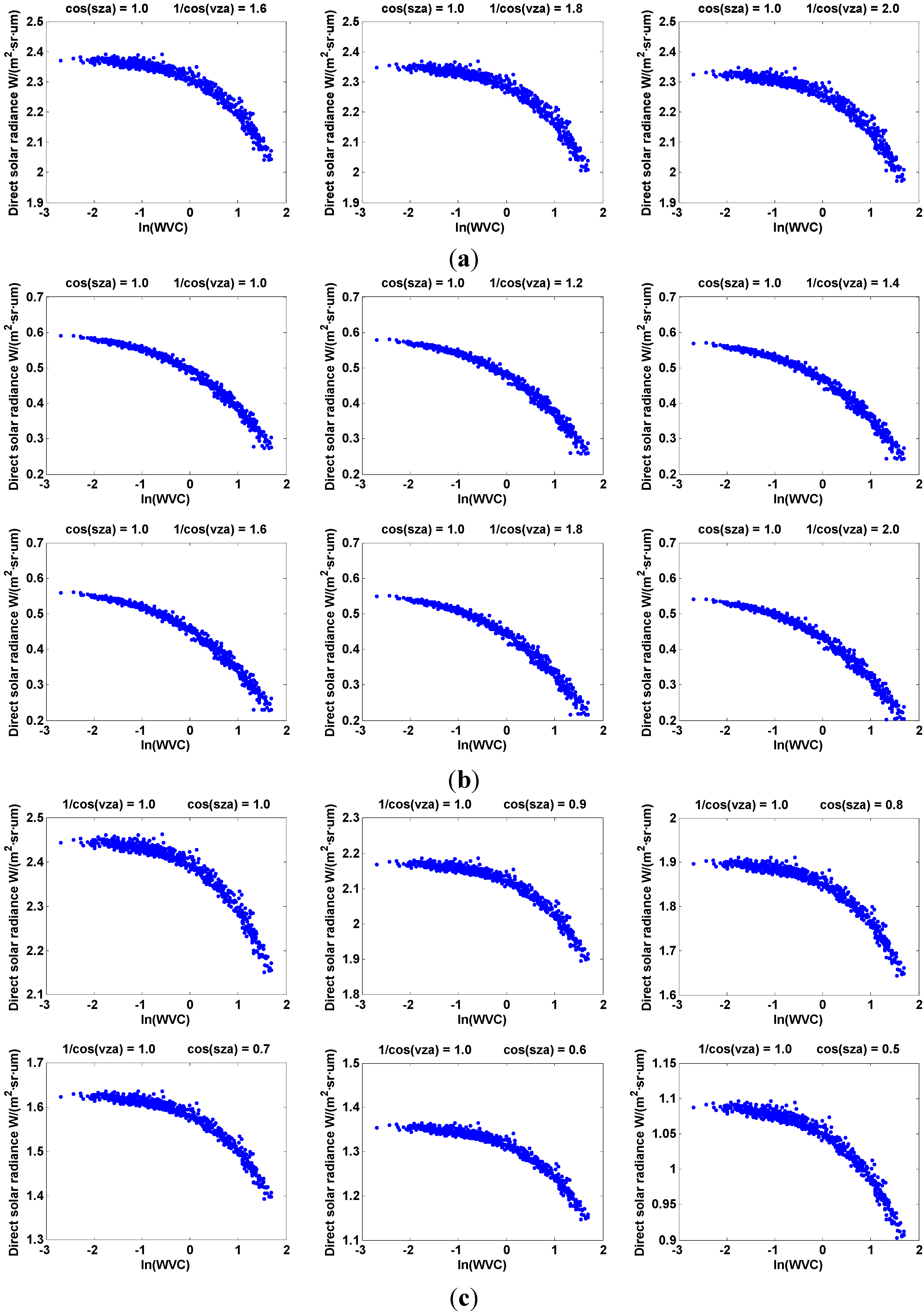
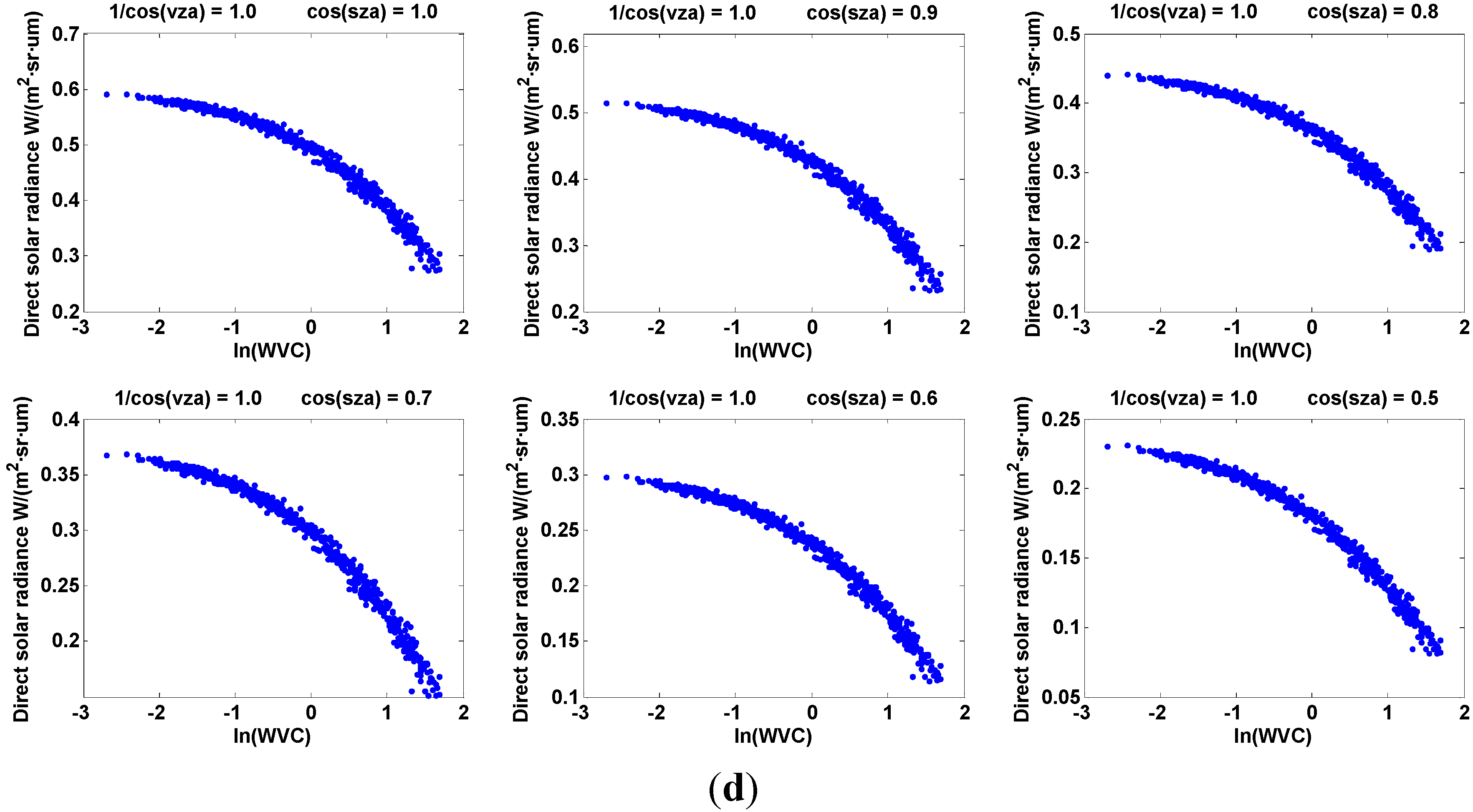
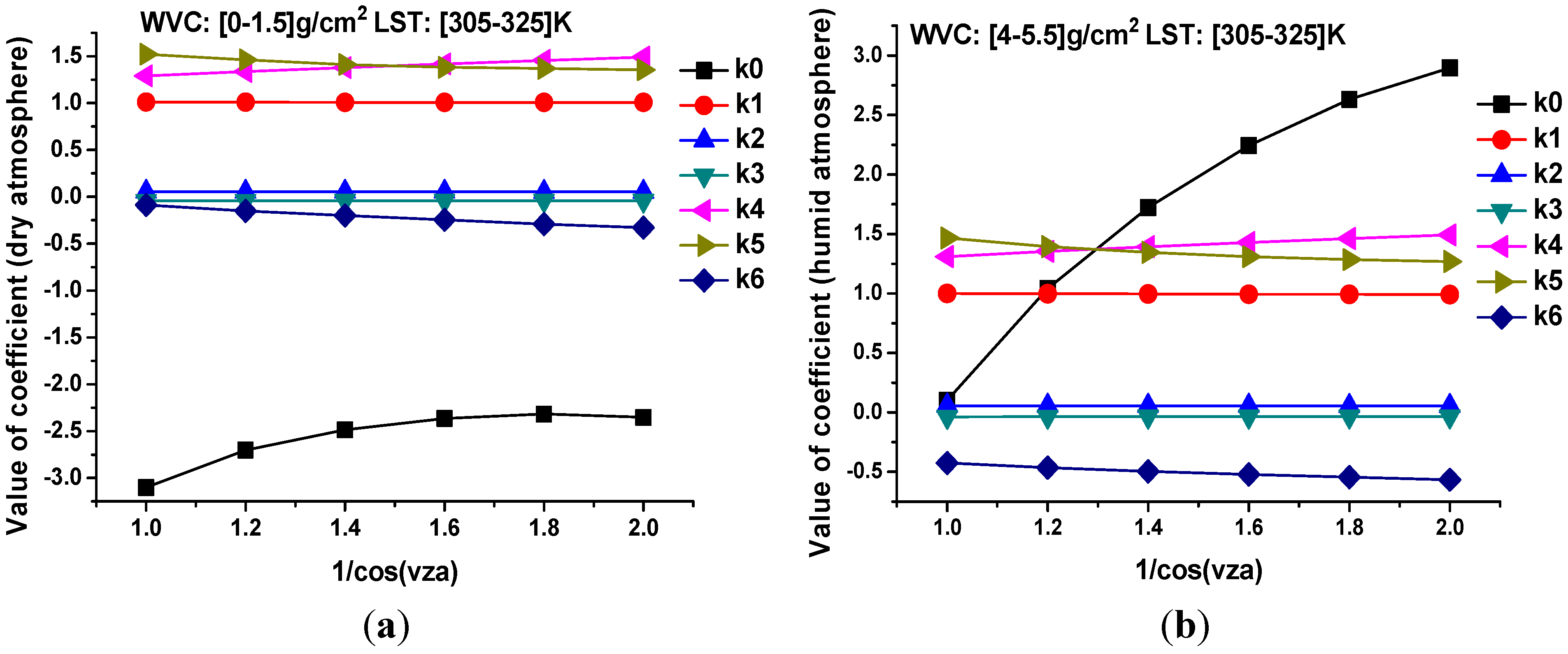
2.3.1. Estimation of Direct Solar Radiance

For the daytime MIR data, estimation of direct solar radiance is premise for LST retrieval because the radiance measured during daytime is strongly affected by the reflected direct solar radiance, which is coupled by the bi-directional reflectivity of the surface (ρbi), the solar radiance at ground level ( R i s ), and the transmittance from ground to sensor ( τ i ). As we all know, τ i is related to WVC and VZA, while R i s is related to WVC and SZA. Therefore, the relationship between direct solar radiance ( D i = τ i × R i s ) and WVC, VZA and SZA is investigated to estimate the direct solar radiance by assuming that the surface is Lambertian and the LSE is known.

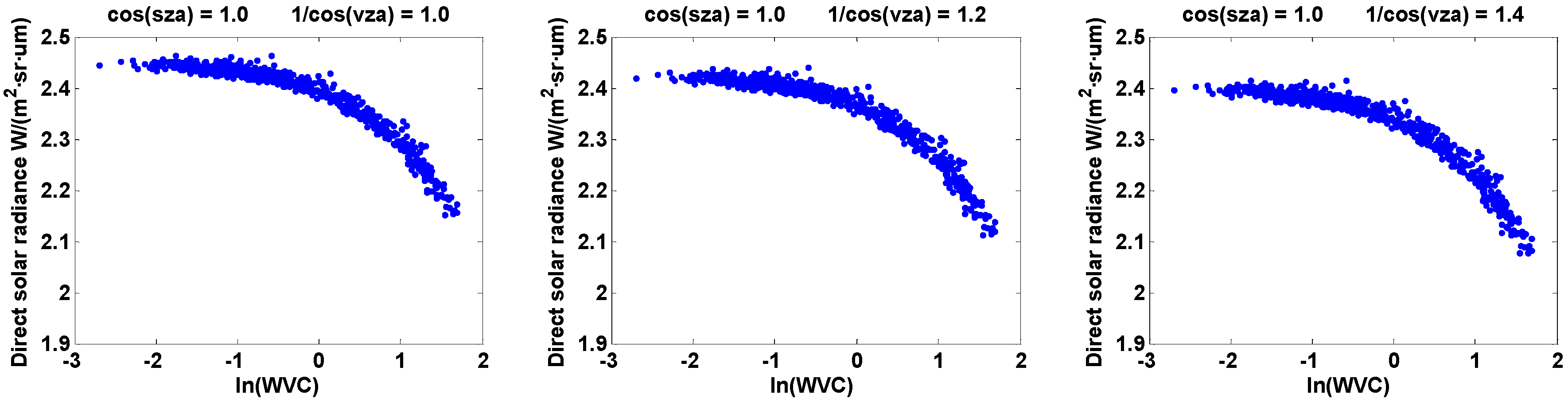
Relationship between Direct Solar Radiance and WVC

To investigate the relationship between Di and WVC with the aid of simulated data, a scatter plot between Di and ln(WVC) is shown in Figure 1. The data is shown for CH66 and CH68 with different VZAs and SZAs at the LST conditions of 250~310 K and WVC of 0~5.5 g/cm2. Figure 1a,b shows the relationships at the six different VZAs when SZA = 0°, while Figure 1c,d shows those at six different SZAs when VZA = 0°. It is noted that Di and ln(WVC) can be fitted using a quadratic polynomial with a formula as Equation (3) with a correlation coefficient of 0.985. Similar results also can be obtained for other combinations of SZAs and VZAs.
D i = a + b ln ( W V C ) + c [ ln ( W V C ) ] 2
where a, b and c are the fitting coefficients. Di is the direct solar radiance.
Figure 1. Relationships between direct solar radiance (Di) and ln(WVC). (a) AHS CH66 (SZA = 0°, VZA = 0~60°). (b) AHS CH68 (SZA = 0°, VZA = 0~60°). (c) AHS CH66 (VZA = 0°, SZA = 0~60°). (d) AHS CH68 (VZA = 0°, SZA = 0~60°).
Remotesensing 06 12667 g001aRemotesensing 06 12667 g001bRemotesensing 06 12667 g001c

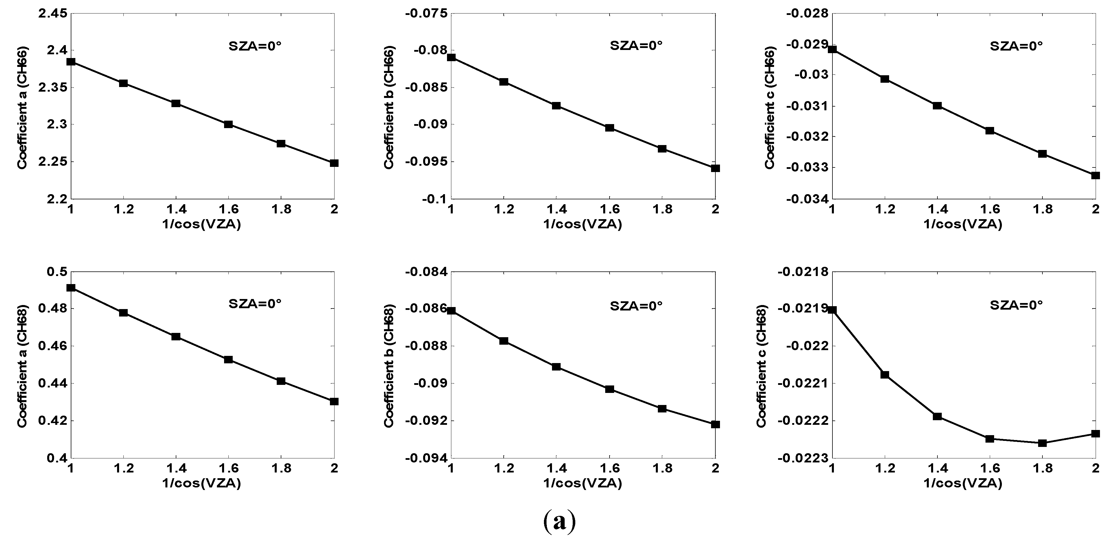
Direct Solar Radiance at Different VZAs

To analyse the effect of VZA on Di, Figure 2a,b express the relationships between coefficients a, b, c and 1/cos(VZA) at SZA = 0° and SZA = 60°, respectively. It is found that the coefficients a, b, and c can be fitted using the formulations of a = a1/cos(VZA) + a2, b = b1/cos(VZA) + b2, and c = c1/cos(VZA) + c2. The direct solar radiance can be described as a function of WVC and VZA as Equation (4) with a correlation coefficient of 0.992.
D i = [ a 1 + a 2 cos ( V Z A ) ] + [ b 1 + b 2 cos ( V Z A ) ] × ln ( W V C ) + [ c 1 + c 2 cos ( V Z A ) ] × [ ln ( W V C ) ] 2
where a1, a2, b1, b2, c1, and c2 are unknown coefficients.
Figure 2. Relationships between coefficients a, b, c and 1/cos(VZA). (a) SZA = 0°. (b) SZA = 60°.
Remotesensing 06 12667 g002aRemotesensing 06 12667 g002b

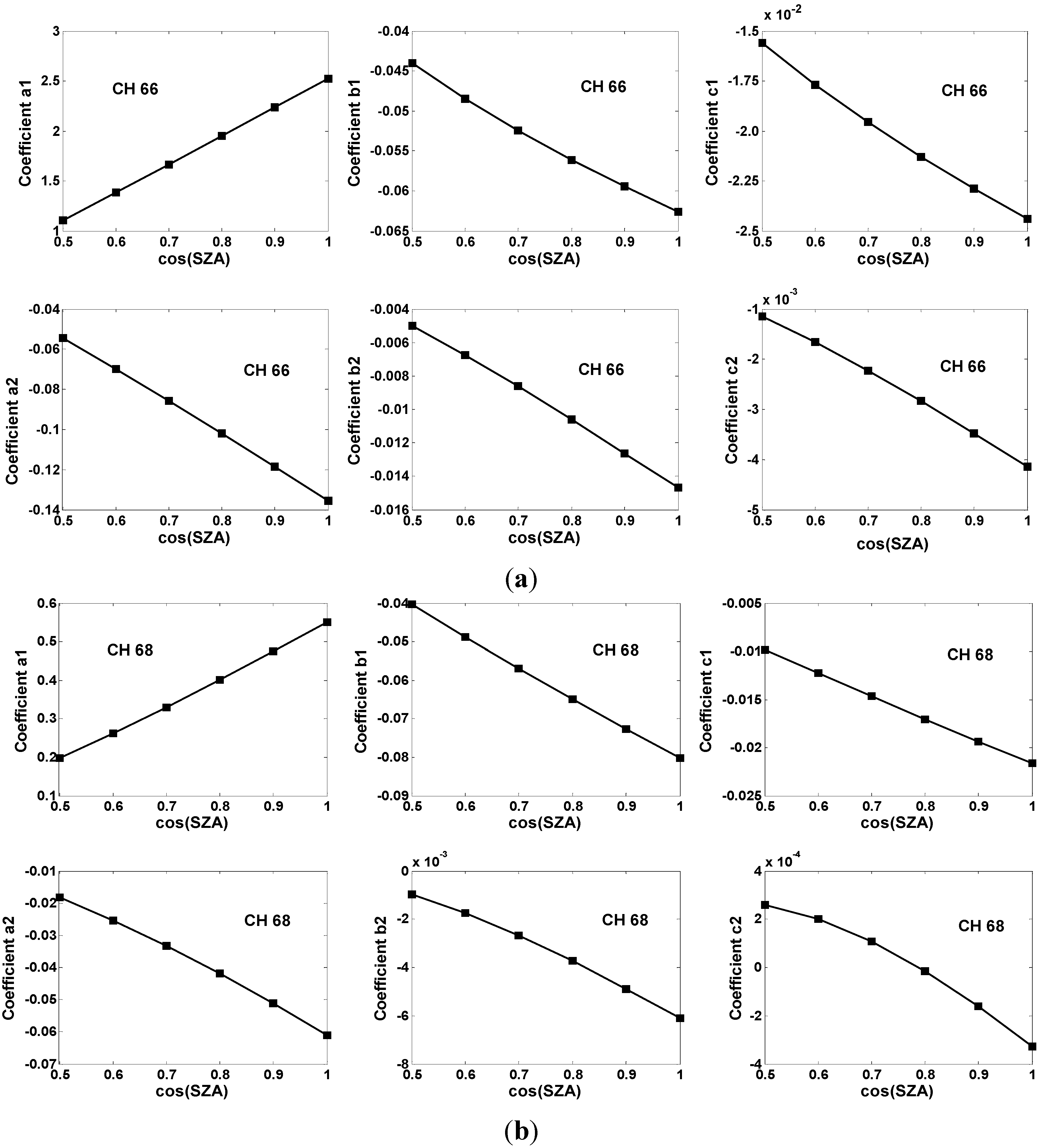
Direct Solar Radiance at Different SZAs

To acquire Di at other SZAs, Figure 3a,b shows the relationships between coefficients a1, a2, b1, b2, c1, c2 and cos(SZA) in CH66 and CH68, respectively. It can be found that these coefficients a1, a2, b1, b2, c1, and c2 can be expressed as a linear relationship of the cosine of SZA, i.e., a1 = a11 cos(SZA) + a10, a2 = a21 cos(SZA) + a20, b1 = b11 cos(SZA) + b10, b2 = b21 cos(SZA) + b20, c1 = c11 cos(SZA) + c10, and c2 = c21 cos(SZA) + c20. Di can be described as a function of WVC, VZA, and SZA as Equation (5) with a correlation coefficient of 0.994.
D i = [ ( a 11 cos ( S Z A ) + a 10 ) + a 21 cos ( S Z A ) + a 20 cos ( V Z A ) ] + [ ( b 11 cos ( S Z A ) + b 10 ) + b 21 cos ( S Z A ) + b 20 cos ( V Z A ) ] × ln ( W V C ) + [ ( c 11 cos ( S Z A ) + c 10 ) + c 21 cos ( S Z A ) + c 20 cos ( V Z A ) ] × [ ln ( W V C ) ] 2
where a11, a10, a21, a20, b11, b10, b21, b20, c11, c10, c21, and c20 are fitting coefficients.

2.3.2. Estimation of LST

Based on the differential absorption (especially for WVC) in two TIR channels in 10~12.5 μm, a split-window method was improved for LST retrieval from TIR data by expressing LST as a linear function of the brightness temperatures Ti and Tj measured in the two adjacent TIR channels [14,15]. In consideration of the similar RTEs in MIR and TIR without the influence of solar direct radiance, this paper extends the split-window method to the MIR spectral region for LST retrieval after eliminating the effect of direct solar radiance. The new method is expressed as follows:
T s = k 0 + ( k 1 + k 2 1 ε ε + k 3 Δ ε ε 2 ) T i + T j 2 + ( k 4 + k 5 1 ε ε + k 6 Δ ε ε 2 ) T i T j 2
where ε = (εi + εj)/2, Δε = εiεj, and k0, k1, k2, k3, k4, k5, and k6 are unknown coefficients, which can be derived from simulated AHS data. T i and T j are the TOA equivalent brightness temperatures in two MIR channels. εi and εj are the LSEs in channel i and j, respectively. ε is the averaged emissivity, and Δε is the emissivity difference between the two MIR channels.
Figure 3. Relationship between coefficients a1, a2, b1, b2, c1, c2 and cos(SZA). (a) AHS CH66. (b) AHS CH68.
Remotesensing 06 12667 g003

3. Results and Analysis

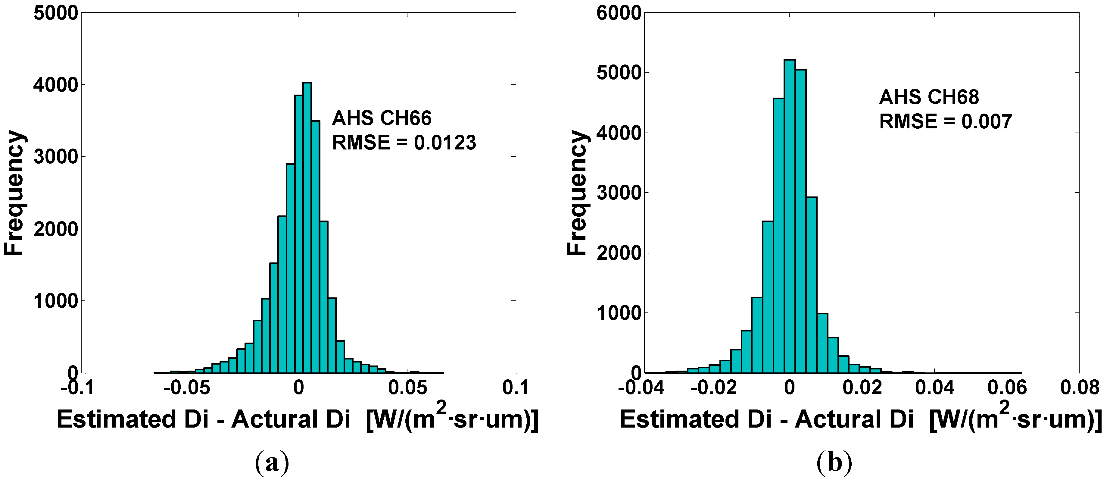
3.1. Estimated Result of Direct Solar Radiance

The above analyses show that Di can be expressed as a function of WVC, SZA and VZA, and the fitting coefficients can be obtained using the simulated data (see Table 1). To evaluate the accuracy of direct solar radiance retrieval, Figure 4a,b shows the histograms of the difference between the estimated and actual Di in CH66 and CH68, respectively. The root mean square errors (RMSEs) are 0.0123 W/(m2·sr·μm) for CH66 and 0.007 W/(m2·sr·μm) for CH68. The correlation coefficients (R) are 0.999 and 0.998, respectively.
Table 1. Fitting coefficients for the direct solar radiance estimation.
Channel Coefficienta11a10a21a20b11b10b21b20c11c10c21c20
AHS CH662.849−0.325−0.1620.028−0.037−0.026−0.0200.005−0.018−0.007−0.0060.002
AHS CH680.709−0.163−0.0860.026−0.080−0.001−0.0100.004−0.0240.002−0.0010.001
Figure 4. Histogram of the difference between the estimated and actual direct solar radiance (Di) for CH66 (a) and CH68 (b).
Remotesensing 06 12667 g004

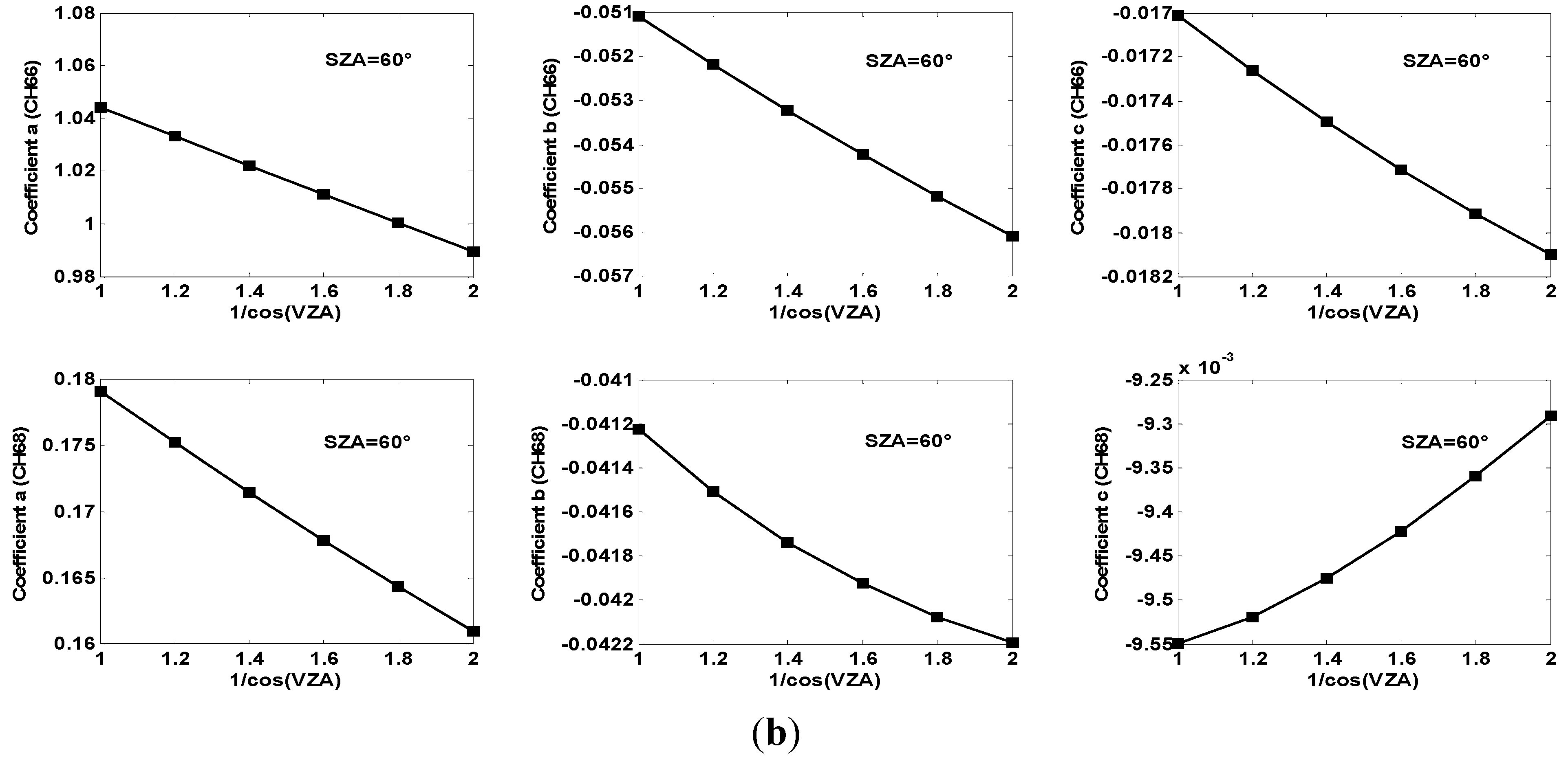
3.2. Coefficients of LST Retrieval Method

After eliminating the effect of direct solar radiance, WVC and LST are divided into several tractable sub-ranges to improve the accuracy of LST retrieval. WVCs are divided into five sub-ranges: [0–1.5], [1–2.5], [2–3.5], [3–4.5], and [4–5.5] g/cm2, and LSTs are divided into three sub-ranges: 265 K ≤ LST ≤ 295 K, 290 K ≤ LST ≤ 310 K, and 305 K ≤ LST ≤ 325 K [31]. Then, the coefficients in Equation (6) can be obtained through a statistical regression method for each sub-range under different VZAs. As an example, Figure 5 displays the coefficients as functions of the secant of VZAs at the sub-ranges of LSTs, which vary from 305 K to 325 K, for the two WVC groups. The coefficients k0~k6 for other VZAs can be linearly interpolated as function of the secant of VZA. Similar results are obtained for the other sub-ranges.
Figure 5. Coefficients for the sub-range with LST varying from 305 K to 325 K. (a) Dry atmosphere (WVC = 0~1.5 g/cm2). (b) Humid atmosphere (WVC = 4~5.5 g/cm2).
Remotesensing 06 12667 g005

3.3. Result of LST Retrieval

In practice, three steps are needed to retrieve LST. First, direct solar radiance is estimated with Equation (5). Second, approximate LSTs are estimated according to Equation (6) with the coefficients derived for the whole range of LST (provided that the sub-ranges of emissivity and WVC are known). Finally, more accurate LSTs are estimated using Equation (6) but with the coefficients k0~k6 of the LST sub-range that is determined according to the approximate LST. Figure 6 gives the RMSEs between the actual and estimated LST as functions of the secant of VZA for different sub-ranges. The RMSEs are shown to increase with the increase of VZAs. The RMSEs are less than 1 K for all sub-ranges; the minimum value is 0.16 K (LST = 305~325 K, WVC = 4~5.5 g/cm2, and VZA = 0°).
Figure 6. RMSEs between the actual and estimated LST for different sub-ranges. (a) 305 K ≤ LST ≤ 325 K. (b) 290 K ≤ LST ≤ 310 K. (c) 265 K ≤ LST ≤ 295 K. (d) 265 K ≤ LST ≤ 325 K.
Remotesensing 06 12667 g006aRemotesensing 06 12667 g006b

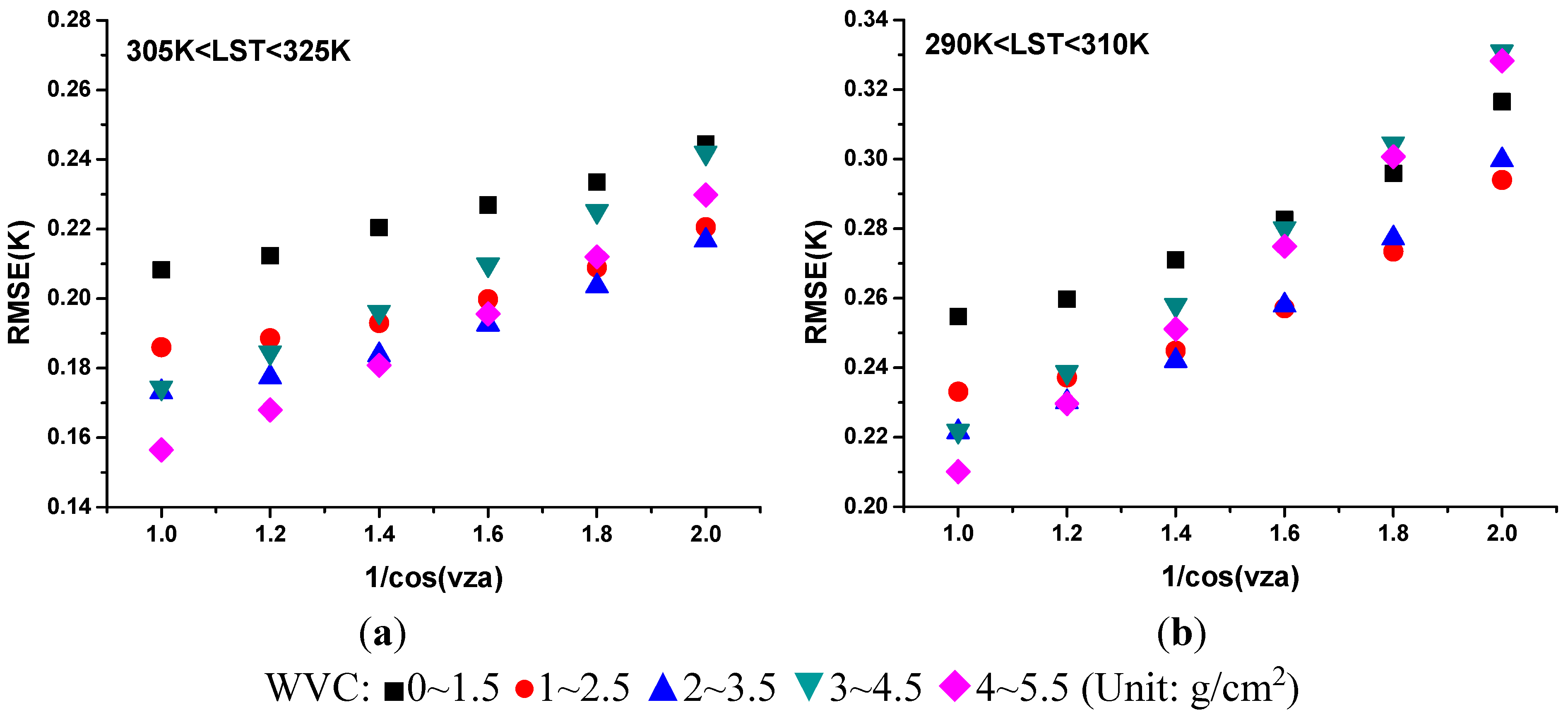
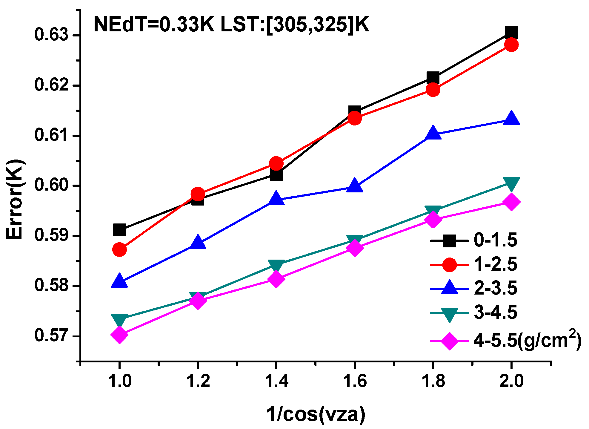
4. Sensitivity Analysis

LST retrieval accuracy is affected by several factors such as the instrumental noises, uncertainties of LSEs and atmospheric properties, and the uncertainty of the method. In this study, the instrument noises (Noise Equivalent difference Temperature, NEΔT), the uncertainties of LSEs and WVCs are taken into account.

4.1. Sensitivity Analysis to Instrumental Noises

The expected NEΔT in AHS channels 66 and 68 is approximately 0.33 K [32]. To analyse the effect of NEΔT on the LST retrieval using Equation (6), a Gaussian random distribution error of 0.33 K is added to the TOA brightness temperatures in CH66 and CH68 in Equation (1). Also, the errors between the LSTs retrieved from the noise-added brightness temperatures and those determined from the noise-free brightness temperatures for the sub-ranges of LST varying from 305 K to 325 K in the five WVC sub-ranges are shown in Figure 7. The results show that the NEΔT of 0.33 K produces approximately an error within 0.63 K when LST is varying from 305 K to 325 K.
Figure 7. LST retrieval error caused by NEΔT when LST is varying from 305 K to 325 K.
Remotesensing 06 12667 g007

4.2. Sensitivity Analysis to LSEs

To analyse the effect of the LSE uncertainty, a Gaussian random distribution error, where the mean of the distribution is 0 and the standard deviation is 0.01, is added to emissivities εi and εj in Equation (6). Table 2 shows the effect of emissivity on the accuracy of LST retrieval at the condition of VZA = 0°. It is worth noting the LST retrieval errors (the LSTs retrieved from LSE-uncertainty-added conditions minus those determined from no-LSE-uncertainty conditions) vary from 0.4 K to 2.83 K by assuming that the uncertainty of the emissivity is 0.01; errors increase with the decrease of LSTs. The reason may be that the proportion of direct solar radiance is larger in the total radiance when the LST is lower, and the same emissivity error may produce a larger effect on TOA radiance with lower LSTs. Meanwhile, the retrieval accuracy will be increasing with the increase of WVC. The possible reason is that the impact of the atmosphere on LST retrieval is more significant when the WVC increases; thus, the same emissivity error would produce smaller errors when the WVC is larger.
Table 2. Effect of the emissivity uncertainty (Δε = 0.01) on LST retrieval.
WVC
(g/cm2)
305~325 (K)
Error
290~310 (K)
Error
265~295 (K)
Error
265~325 (K)
Error
0~1.50.501.042.832.71
1~2.50.490.941.681.31
2~3.50.440.841.370.92
3~4.50.400.761.400.81
4~5.50.400.741.260.73

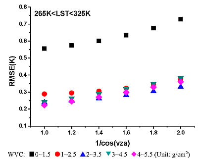
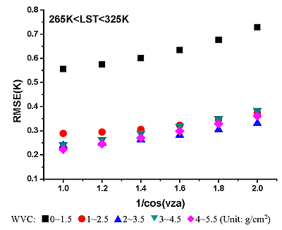
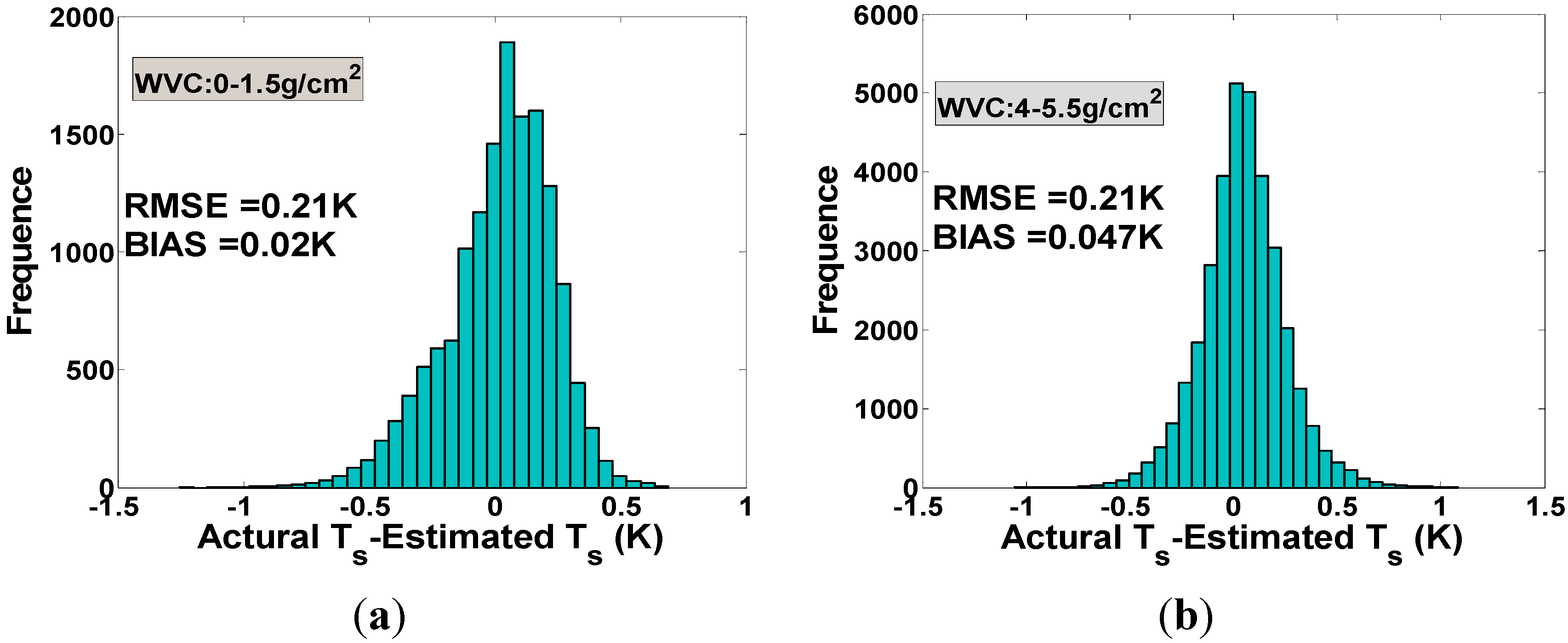
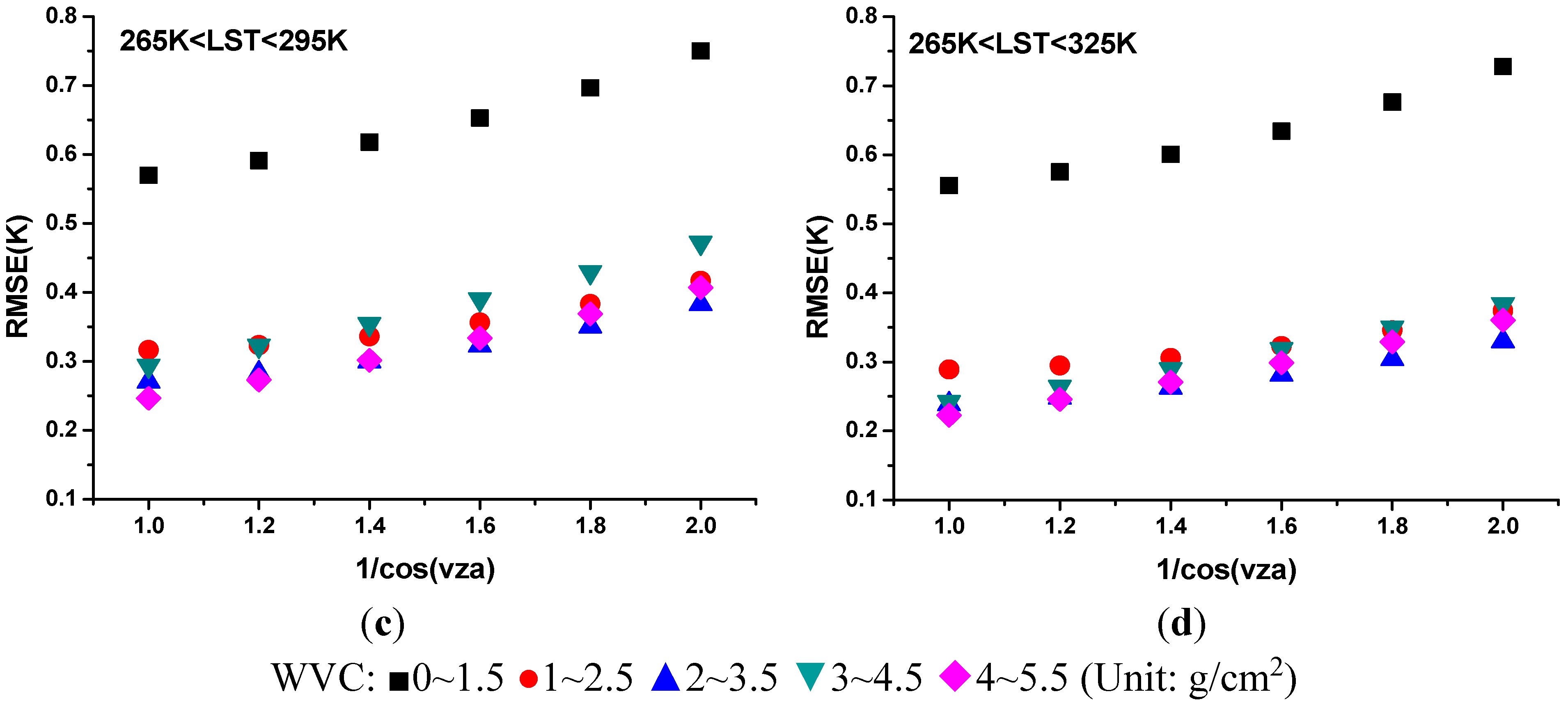
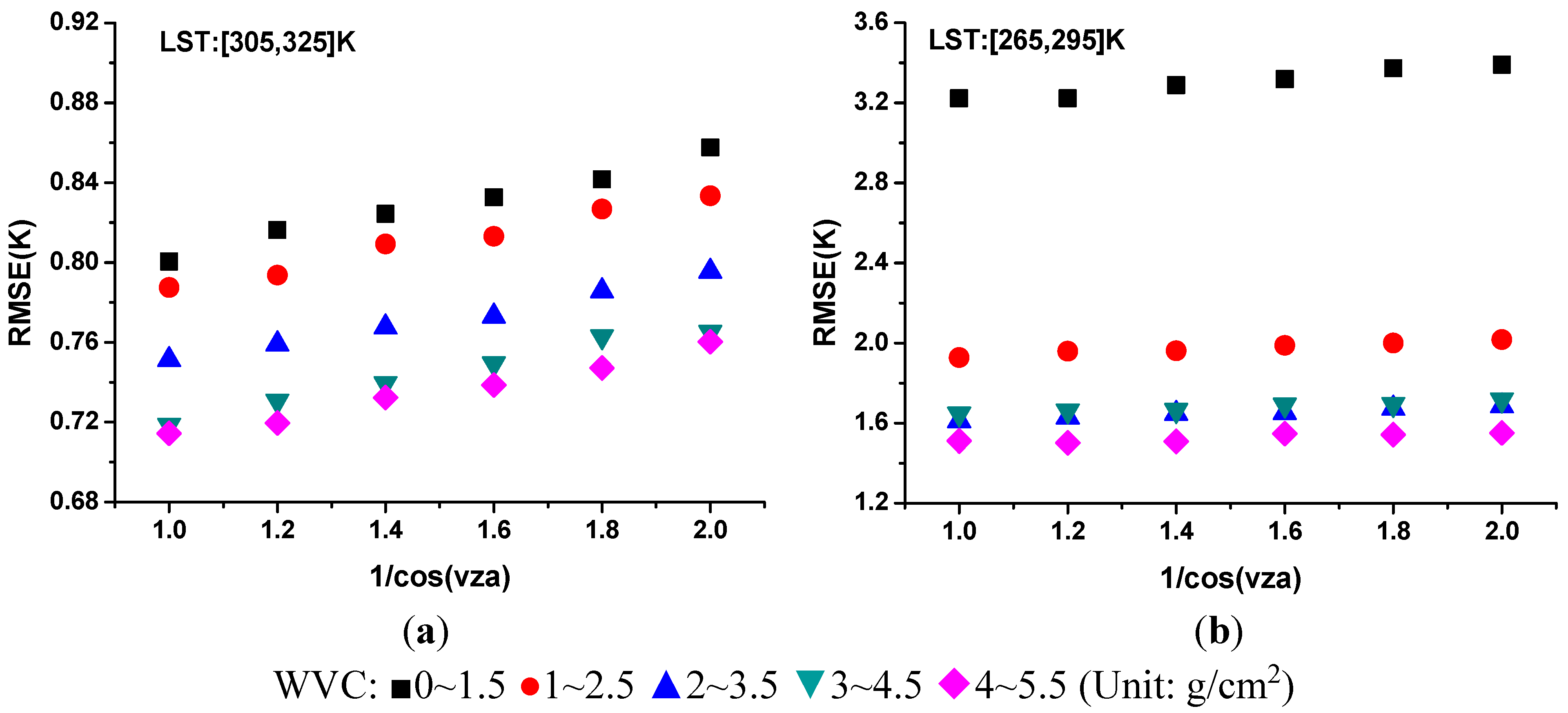
4.3. Sensitivity Analysis to WVC

To investigate how significant is the effect of the uncertainty of the WVC on the retrieval of LST, a Gaussian random distribution error, where the mean of the distribution is 0 and the standard deviation is 10%, is added to WVC. The WVC error will affect the accuracy of direct solar radiance estimation and cause the wrong selection of sub-range retrieval coefficients. Figure 8a,b shows the histograms of LST errors caused by a WVC uncertainty of 10% under the conditions of VZA = 0°, LST = 305~325 K, and atmospheric WVC = 0~1.5 g/cm2 (dry atmosphere) or 4~5.5 g/cm2 (wet atmosphere). It can be seen from Figure 8 that RMSE and Bias are 0.21 K and 0.02 K under dry atmosphere, respectively, and 0.21 K and 0.047 K under wet atmosphere, respectively.
Considering the instrument noises ( sin ( θ ) = cos ( h ) cos ( δ ) cos ( φ ) + sin ( δ ) sin ( φ ) ), the uncertainties of LSEs ( δ ( L S T ε ) ) and WVC ( δ ( L S T W V C ) ), and the accuracy of the algorithm ( δ ( L S T r ) ), the overall error on the LST ( δ ( L S T ε ) ) can be described by the following:
δ ( L S T ) = δ 2 ( L S T r ) + δ 2 ( L S T ε ) + δ 2 ( L S T N E Δ T ) + δ 2 ( L S T W V C )
Inserting the δ ( L S T r ) values illustrated in Figure 6 for sub-ranges of LST = 305~325 K and LST = 265~295 K at all combinations of VZAs and WVCs, the overall δ ( L S T ) error is shown in Figure 9. Figure 9 shows that the biggest RMSE is approximately 3.39 K for the sub-range of LST = 265~295 K and WVC = 0~1.5 g/cm2 at VZA = 60°. The smallest RMSE is approximately 0.72 K for the sub-range of LST = 305~325 K and WVC = 4~5.5 g/cm2 at VZA = 0°.
Figure 8. Histogram of the difference between the actual and estimated Ts caused by a WVC uncertainty of 10%. (a) WVC = 0~1.5 g/cm2. (b) WVC = 4~5.5 g/cm2.
Remotesensing 06 12667 g008
Figure 9. Total LST retrieval error caused by uncertainties of NEΔT, emissivity, and WVC. (a) High LST conditions (LST = 305~325 K). (b) Low LST conditions (LST = 265~295 K).
Remotesensing 06 12667 g009

5. Preliminary Application to AHS data

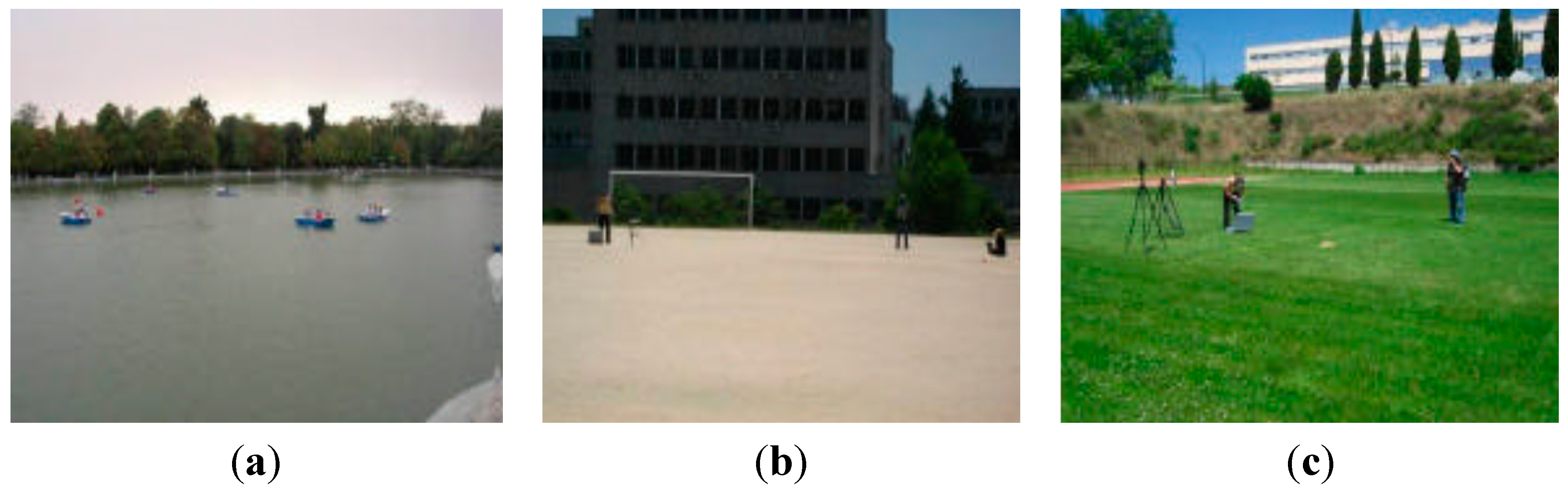
5.1. Data Processing

The AHS instrument has 80 spectral bands covering the visible and near infrared (VNIR), short wave infrared (SWIR), mid-infrared (MIR), and thermal infrared (TIR) spectral ranges. The instrument is operated by Instituto Nacional de Técnica Aerospacial (INTA) and it has been involved in several field campaigns since 2004. The arrangement of the AHS mid-infrared bands covered by 3.3~5.4 µm has seven bands (i.e., CH 64 ~CH 70), and its bandwidth is 35 nm with λ/∆λ (minimum) of 110 [33]. In this study, the proposed method is applied to AHS data collected on 4 July 2008 over a study area in the city and suburbs of Madrid covered by vegetation, water, buildings, roads, bare soil, etc.
Due to the influence of the attitude and speed of the spacecraft and the Earth’s rotation, the AHS image would emerge a certain degree of geometric distortions, such as compression, stretching and offset compared to the actual position of the ground target pixels. Hence, to obtain the accurate location of the image pixels, the image geometric correction is carried out using the module of IGM in ENVI 4.7 with the aid of the geographic coordinate of each pixel. Then, the SZA for every pixel can be calculated using Equation (8) with the information of latitude and longitude, while the VZA of each pixel can be acquired according to the field of view (FOV) of the AHS sensor (90°) and the pixel numbers.
sin ( θ ) = cos ( h ) cos ( δ ) cos ( ϕ ) + sin ( δ ) sin ( ϕ )
where θ is the solar zenith angle. h is the hour angle at the local sidereal system. δ is the solar declination. φ is the local latitude.
Because it is difficult to obtain the ground measured LSEs in practice, the LSEs are determined using the supervised classification methods with the VNIR hyperspectral data equipped on the AHS sensor. Five categories, i.e., grass, water, roads, houses and bare soil, have been classified. The LSEs in AHS CH 66 and CH 68 are obtained by integrating emissivity spectral curves extracted from the JHU library with the spectral response function. In addition, WVC is extracted from the radiosonde atmospheric profiles acquired at the imaging time (approximately 0.76 g/cm2).

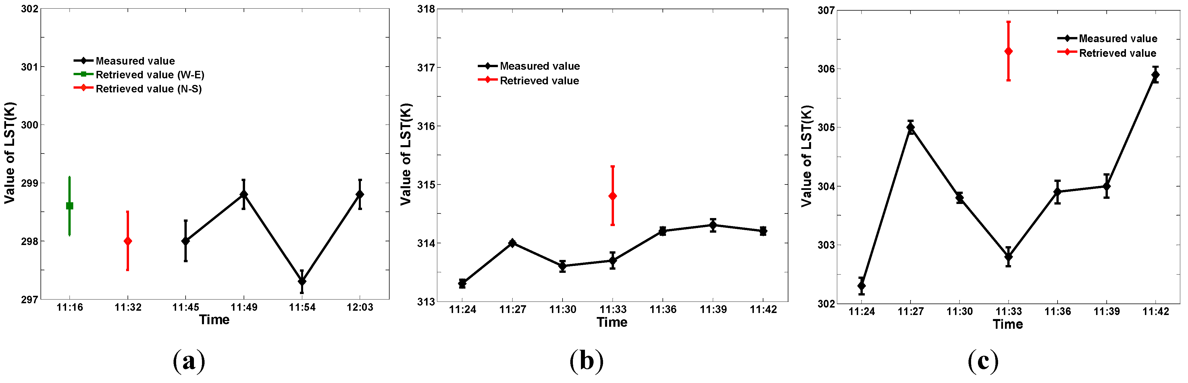
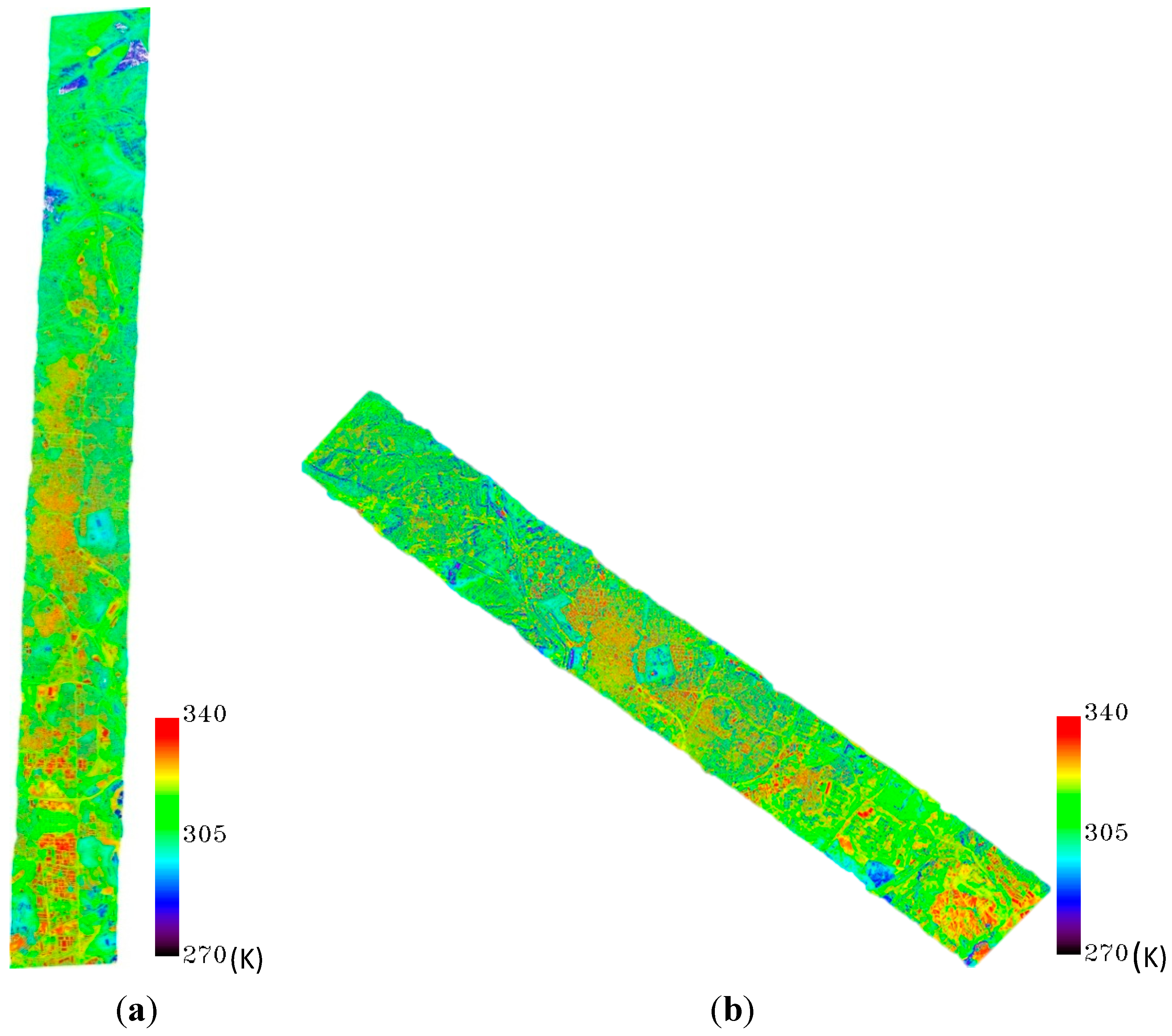
5.2. Results and Validation

After data processing, the LSTs can be derived using Equation (6) from AHS MIR data on 4 July 2008 (N-S data 11:32 and W-E data at 11:16, both are at 2497 m with scan-rate 18.7 rpt, see Figure 10a,b). The selected surfaces for validation were (see Figure 11): (i) Water body, as cold target, in the lake at “El Retiro” park (40°25'1.65"N, 3°41'2.65"W), (ii) Bare soil, as hot target, in the soccer field at UAM (40°32'52.44"N, 3°41'48.45"W), (iii) Green grass, as cold target, in the Rugby field at UAM (40°32'51.71"N, 3°41'54.33"W). The in situ measurements were carried out making transects at regular steps in representative and vast surfaces during the flight overpasses. Various instruments in the thermal infrared domain were used, including the CIMEL models CE312-1 and CE312-2, Heitronics KT 19.85 and NEC TH9100, whose technical specifications are shown in Table 3 [33].
Table 3. Technical specifications of the thermal instruments [33].
InstrumentSpectral Range (um)Temperature Range (°C)Accuracy (K)ResolutionFOV
Cimel CE312-18~13−80 to 500.18 mK10°
11.5~12.550 mK
10.5~11.550 mK
8.2~9.250 mK
Cimel CE312-28~13−80 to 600.18 mK10°
11~11.750 mK
10.3~1150 mK
8.9~9.350 mK
8.5~8.950 mK
8.1~8.550 mK
Heitronics KT199.6~11.5−50 to 2000.10.05 K
NEC TH91008~14−40 to 12020.1 K
(320 × 240)
22° × 16°
Figure 10. LST retrieval for AHS data. (a) LST of AHS (N-S) (b) LST of AHS (W-E).
Remotesensing 06 12667 g010
Figure 11. Three areas with different covering types. (a) Retiro Park (water). (b) Soccer field (bare soil). (c) Football field (grass) [33].
Remotesensing 06 12667 g011
For each validation area, the LSTs of the 2 × 2 pixels nearest to the geographic coordinate of the in situ measurement are selected. The estimated average LST of the four pixels is compared with the average of in situ measurements acquired within 5 minutes. The differences between estimated and measured LST for the three areas are approximately 0.7 K, 0.9 K, and 2.3 K (see Table 4). The vegetation area presents a larger LST retrieval error, which would be caused by its larger bias of measured LST (the bias is approximately 2 K, see Figure 12) due to the nonuniformity of the grass area covered by grass and soil; whereas, water and bare soil received better results because the compositions of water and bare soil are relatively uniform.
Table 4. Validation results over three areas.
CoordinateSurface TypeLSERetrieved LSTIn situ MeasurementIn situ Bias
ε66ε68
40°25′1.65″N, 3°41′2.65″WWater0.9760.979297.6K298.3K0.3K
40°32′52.44″N, 3°41′48.45″WBare soil0.7690.799314.8K313.9K0.6K
40°32′51.71″N, 3°41′54.33″WGrass0.9840.987306.3K304.0K2K
Figure 12. Validation results over three areas. (a) Retiro Park (water). (b) Soccer field (bare soil). (c) Football field (grass).
Remotesensing 06 12667 g012

6. Conclusions

In this study, a new algorithm for LST retrieval from daytime AHS data in two MIR channels, CH66 and CH68, is proposed. In this method, to retrieve LST more accurately, the atmospheric WVC and the LST are divided into several tractable sub-ranges. The coefficients of each sub-range in the algorithm are calculated using a statistical regression method from the numerical values simulated with the atmospheric radiative transfer model MODTRAN 4.0 under different atmospheric and surface conditions. The simulation analysis shows that the LST could be estimated by this algorithm with the RMSE less than 1 K for all of the sub-ranges with the knowledge of the LSEs.
In addition, the sensitivity analysis is performed in terms of the instrumental noise, the uncertainty of the LSE and WVC. The results show that, for the sub-range with VZA = 0° and LST = 305~325 K, an instrumental error of 0.33 K would produce a LST retrieval error of 0.6 K; the LST error caused by an LSE uncertainty of 0.01 varies from 0.4 K to 2.8 K. A LST retrieval error of approximately 0.2 K is caused by the WVC uncertainty of 10%. The largest total uncertainty is approximately 3.39 K for the sub-range of LST = 265~295 K and WVC = 0~1.5 g/cm2 at VZA = 60°. The smallest one is approximately 0.72 K for the sub-range of LST = 305~325 K and WVC = 4~5.5 g/cm2 at VZA = 0°.
Finally, the proposed LST retrieval algorithm is applied to the AHS data and is validated over three land surface types with in situ measurements. The validation results show that the differences between estimated and measured LST for water, bare soil and grass areas are approximately 0.7 K, 0.9 K, and 2.3 K, respectively.

Acknowledgments

This work has been supported by the National Natural Science Foundation of China under Grants 41371353, 41231170, 41301387, the National Key Basic Research Program under Grants 2013CB733402. The authors would like to thank Sobrino J.A. for providing AHS data. Also, the thanks are given to the anonymous reviewers for their valuable suggestions and comments.

Author Contributions

Enyu Zhao wrote the manuscript and was responsible for the research design, data preparation and analysis. Yonggang Qian, Caixia Gao, and Xiaoguang Jiang conceived and designed the research. Hongyuan Huo and Xiangsheng Kong collected, processed, and analyzed the remotely sensed data.

Conflicts of Interest

The authors declare no conflict of interest.

References and Notes

  1. Hansen, J.; Ruedy, R.; Sato, M.; Lo, K. Global surface temperature change. Rev. Geophys. 2010, 48. [Google Scholar] [CrossRef]
  2. Bastiaanssen, W.; Menenti, M.; Feddes, R.; Holtslag, A. A remote sensing surface energy balance algorithm for land (SEBAL) 1. Formulation. J. Hydrol. 1998, 212, 198–212. [Google Scholar]
  3. Anderson, M.; Norman, J.; Kustas, W.; Houborg, R.; Starks, P.; Agam, N. A thermal-based remote sensing technique for routine mapping of land-surface carbon, water and energy fluxes from field to regional scales. Remote Sens. Environ. 2008, 112, 4227–4241. [Google Scholar] [CrossRef]
  4. Karnieli, A.; Agam, N.; Pinker, R.T.; Anderson, M.; Imhoff, M.L.; Gutman, G.G.; Panov, N.; Goldberg, A. Use of NDVI and land surface temperature for drought assessment: Merits and limitations. J. Climate 2010, 23, 618–633. [Google Scholar] [CrossRef]
  5. Kustas, W.; Anderson, M. Advances in thermal infrared remote sensing for land surface modeling. Agric. Forest Meteorol. 2009, 149, 2071–2081. [Google Scholar] [CrossRef]
  6. Zhang, R.; Tian, J.; Su, H.; Sun, X.; Chen, S.; Xia, J. Two improvements of an operational two-layer model for terrestrial surface heat flux retrieval. Sensors 2008, 8, 6165–6187. [Google Scholar] [CrossRef]
  7. Cho, A.-R.; Suh, M.-S. Evaluation of land surface temperature operationally retrieved from Korean geostationary satellite (COMS) data. Remote Sens. 2013, 5, 3951–3970. [Google Scholar] [CrossRef]
  8. Bechtel, B.; Zakšek, K.; Hoshyaripour, G. Downscaling land surface temperature in an urban area: A case study for hamburg, germany. Remote Sens. 2012, 4, 3184–3200. [Google Scholar] [CrossRef]
  9. Weng, Q. Thermal infrared remote sensing for urban climate and environmental studies: Methods, applications, and trends. ISPRS J. Photogramm. Remote Sens. 2009, 64, 335–344. [Google Scholar] [CrossRef]
  10. Kalma, J.D.; McVicar, T.R.; McCabe, M.F. Estimating land surface evaporation: A review of methods using remotely sensed surface temperature data. Sur. Geophys. 2008, 29, 421–469. [Google Scholar] [CrossRef]
  11. Voogt, J.A.; Oke, T.R. Thermal remote sensing of urban climates. Remote Sens. Environ. 2003, 86, 370–384. [Google Scholar] [CrossRef]
  12. Arnfield, A.J. Two decades of urban climate research: A review of turbulence, exchanges of energy and water, and the urban heat island. Int. J. Climatol. 2003, 23, 1–26. [Google Scholar] [CrossRef]
  13. Su, Z. The surface energy balance system (SEBS) for estimation of turbulent heat fluxes. Hydrol. Earth Syst. Sci. 2002, 6, 85–100. [Google Scholar] [CrossRef]
  14. Kogan, F.N. Operational space technology for global vegetation assessment. Bull. Am. Meteorol. Soc. 2001, 82, 1949–1964. [Google Scholar] [CrossRef]
  15. Li, Z.-L.; Tang, B.-H.; Wu, H.; Ren, H.; Yan, G.; Wan, Z.; Trigo, I.F.; Sobrino, J.A. Satellite-derived land surface temperature: Current status and perspectives. Remote Sens. Environ. 2013, 131, 14–37. [Google Scholar] [CrossRef]
  16. Sobrino, J.; El Kharraz, J.; Li, Z.-L. Surface temperature and water vapour retrieval from MODIS data. Int. J. Remote Sens. 2003, 24, 5161–5182. [Google Scholar] [CrossRef]
  17. Jiménez-Muñoz, J.C.; Sobrino, J.A. A generalized single-channel method for retrieving land surface temperature from remote sensing data. J. Geophys. Res. 2003, 108. [Google Scholar] [CrossRef]
  18. Qin, Z.H.; Karnieli, A.; Berliner, P. A mono-window algorithm for retrieving land surface temperature from landsat tm data and its application to the Israel-Egypt border region. Int. J. Remote Sens. 2001, 22, 3719–3746. [Google Scholar] [CrossRef]
  19. Wan, Z.; Dozier, J. A generalized split-window algorithm for retrieving land-surface temperature from space. IEEE Tran. Geosci. Remote Sens. 1996, 34, 892–905. [Google Scholar] [CrossRef]
  20. Becker, F.; Li, Z.-L. Towards a local split window method over land surfaces. Int. J. Remote Sens. 1990, 11, 369–393. [Google Scholar] [CrossRef]
  21. Li, Z.-L.; Wu, H.; Wang, N.; Qiu, S.; Sobrino, J.A.; Wan, Z.; Tang, B.-H.; Yan, G. Land surface emissivity retrieval from satellite data. Int. J. Remote Sens. 2013, 34, 3084–3127. [Google Scholar] [CrossRef]
  22. Mushkin, A.; Balick, L.K.; Gillespie, A.R. Extending surface temperature and emissivity retrieval to the mid-infrared (3–5 μm) using the multispectral thermal imager (MTI). Remote Sens. Environ. 2005, 98, 141–151. [Google Scholar] [CrossRef]
  23. Salisbury, J.W.; D’Aria, D.M. Emissivity of terrestrial materials in the 3–5 μm atmospheric window. Remote Sens. Environ. 1994, 47, 345–361. [Google Scholar] [CrossRef]
  24. Sun, D.; Pinker, R.T. Estimation of land surface temperature from a geostationary operational environmental satellite (GOES-8). J. Geophys. Res. 2003, 108. [Google Scholar] [CrossRef]
  25. Baker, N. Polar Satellite System (JPSS) VIIRS Land Surface Temperature Algorithm Theoretical Basis Document (ATBD) GSFC JPSS. Available online: http://npp.gsfc.nasa.gov/sciencedocuments/ATBD_122011/474-00051_LandSurfTemp_Rev-_20110422.pdf (accessed on 05 December 2011).
  26. Li, Z.-L.; Petitcolin, F.; Zhang, R. A physically based algorithm for land surface emissivity retrieval from combined mid-infrared and thermal infrared data. Sci. China Series E: Tech. Sci. 2000, 43, 23–33. [Google Scholar]
  27. Sobrino, J.A.; Jiménez-Muñoz, J.C.; Zarco-Tejada, P.J.; Sepulcre-Cantó, G.; de Miguel, E. Land surface temperature derived from airborne hyperspectral scanner thermal infrared data. Remote Sens. Environ. 2006, 102, 99–115. [Google Scholar] [CrossRef]
  28. Chevallier, F.; Chéruy, F.; Scott, N.; Chédin, A. A neural network approach for a fast and accurate computation of a longwave radiative budget. J. Appl. Meteorol. 1998, 37, 1385–1397. [Google Scholar] [CrossRef]
  29. Chedin, A.; Scott, N.A.; Wahiche, C.; Moulinier, P. The improved initialization inversion method: A high resolution physical method for temperature retrievals from satellites of the TIROS-N series. J. Climate appl. Meteorol. 1985, 24, 128–143. [Google Scholar] [CrossRef]
  30. Sobrino, J.A.; Jiménez-Muñoz, J.C.; El-Kharraz, J.; Gómez, M.; Romaguera, M.; Sòria, G. Single-channel and two-channel methods for land surface temperature retrieval from DAIS data and its application to the Barrax site. Int. J. Remote Sens. 2004, 25, 215–230. [Google Scholar] [CrossRef]
  31. Jiang, G.M.; Zhou, W.; Liu, R. Development of split-window algorithm for land surface temperature estimation from the VIRR/FY-3A measurements. IEEE Geosci. Remote Sens. Lett. 2013, 10, 952–956. [Google Scholar] [CrossRef]
  32. Jim#xE9;nez-Muñoz, J.C.; Gómez, J.A.; Fernández-Renau, A.; Holguín, J.A.; de Miguel, E.; de la Cámara, O.G.; Prado, E. Comportamiento geométrico y radiométrico del sensor ahs durante la campaña multitemporal cefles2 geometric and radiometric performance of the ahs sensor along cefles2. Revista de Teledetección 2010, 34, 16–21. [Google Scholar]
  33. Sobrino, J.A. Dual-Use European Security IR Experiment 2008 (DESIREX 2008) Final Report. Available online: https://earth.esa.int/c/document_library/get_file?folderId=21020&name=DLFE-905.pdf (accessed on 24 March 2009).

