The Strengths and Limitations in Using the Daily MODIS Open Water Likelihood Algorithm for Identifying Flood Events


Abstract
:
1. Introduction
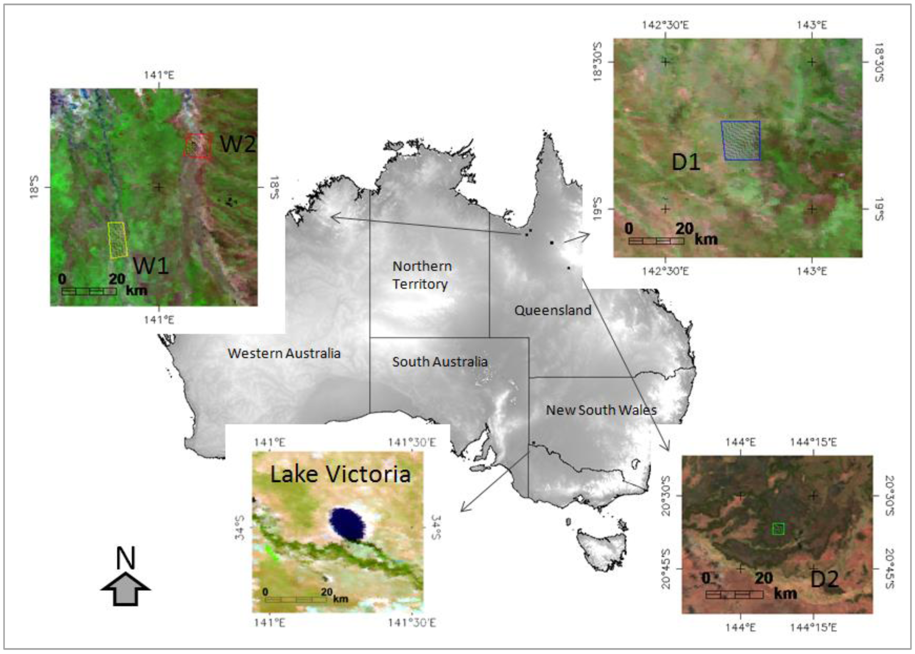
2. Study Sites
3. Data
4. Method
MODIS OWL Water Maps
| β0 = −3.41375620 | |
| β1 = −0.000959735270 | x1 = SWIR band 6 (reflectance*1000) |
| β2 = 0.00417955330 | x2 = SWIR band 7 (reflectance*1000) |
| β3 = 14.1927990 | x3 = NDVI |
| β4 = −0.430407140 | x4 = NDWI (Gao, 1996) |
| β5 = −0.0961932990 | x5 = MrVBFI (Gallant and Dowling, 2003) |
5. Results
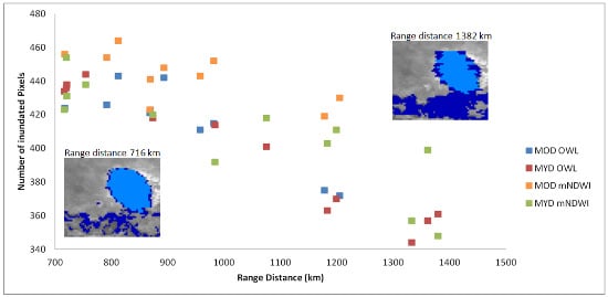
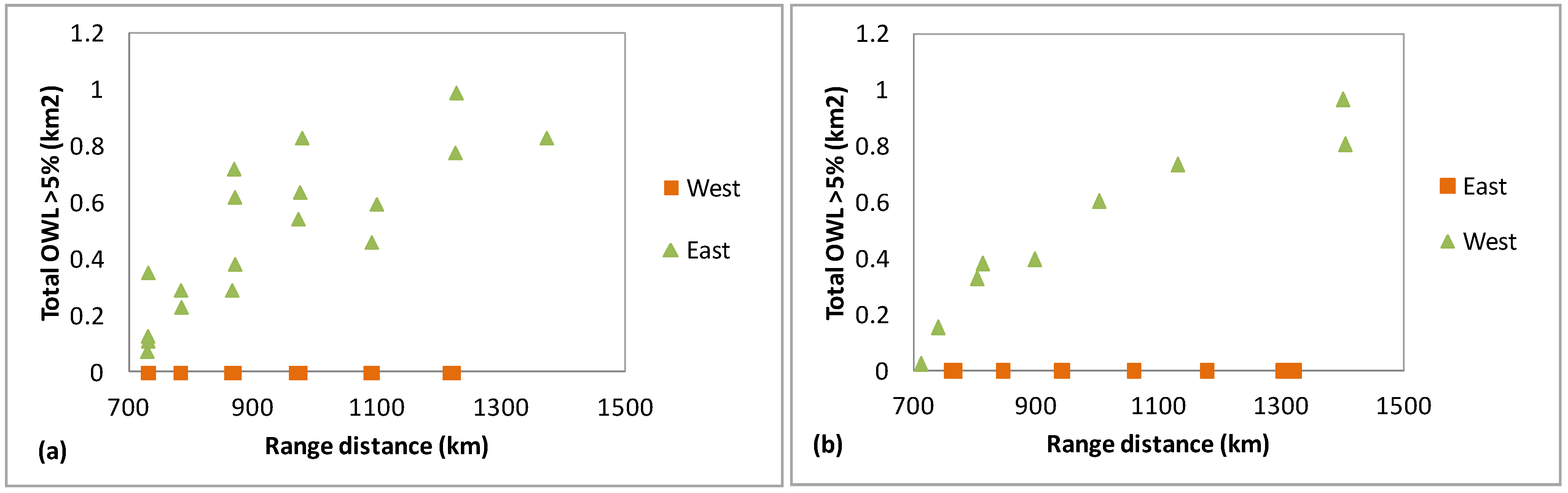
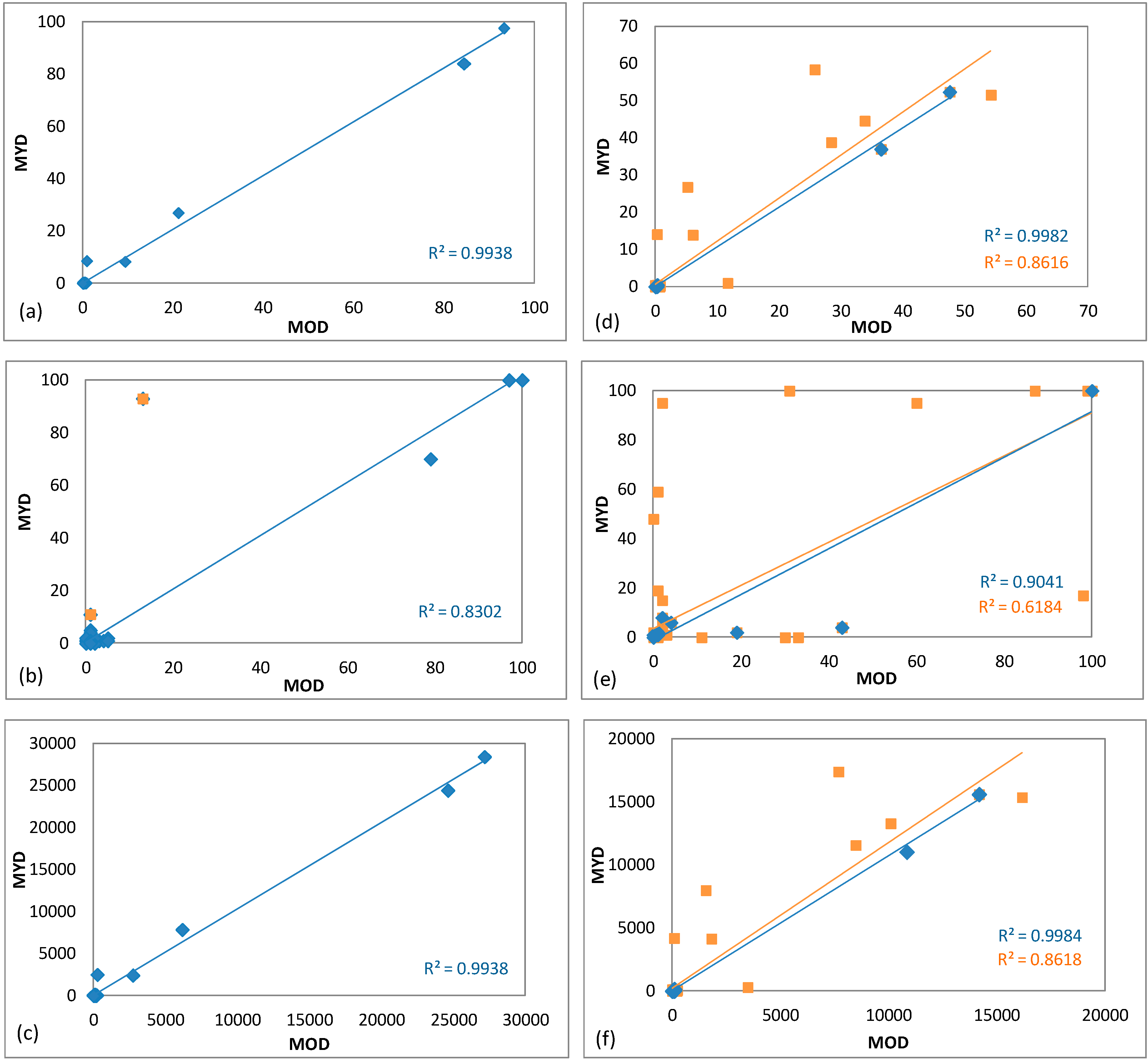
5.1. Relationship between MODIS OWL and View Angle of a Permanent Water Body
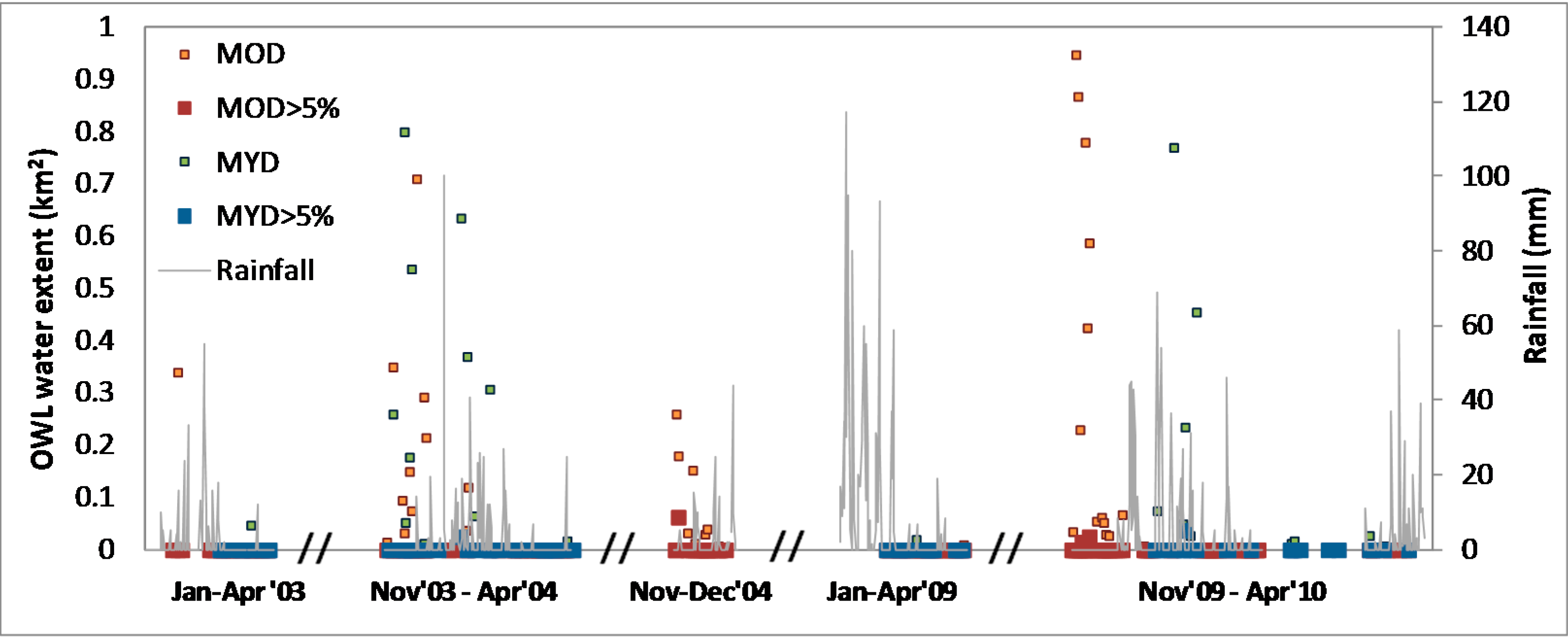
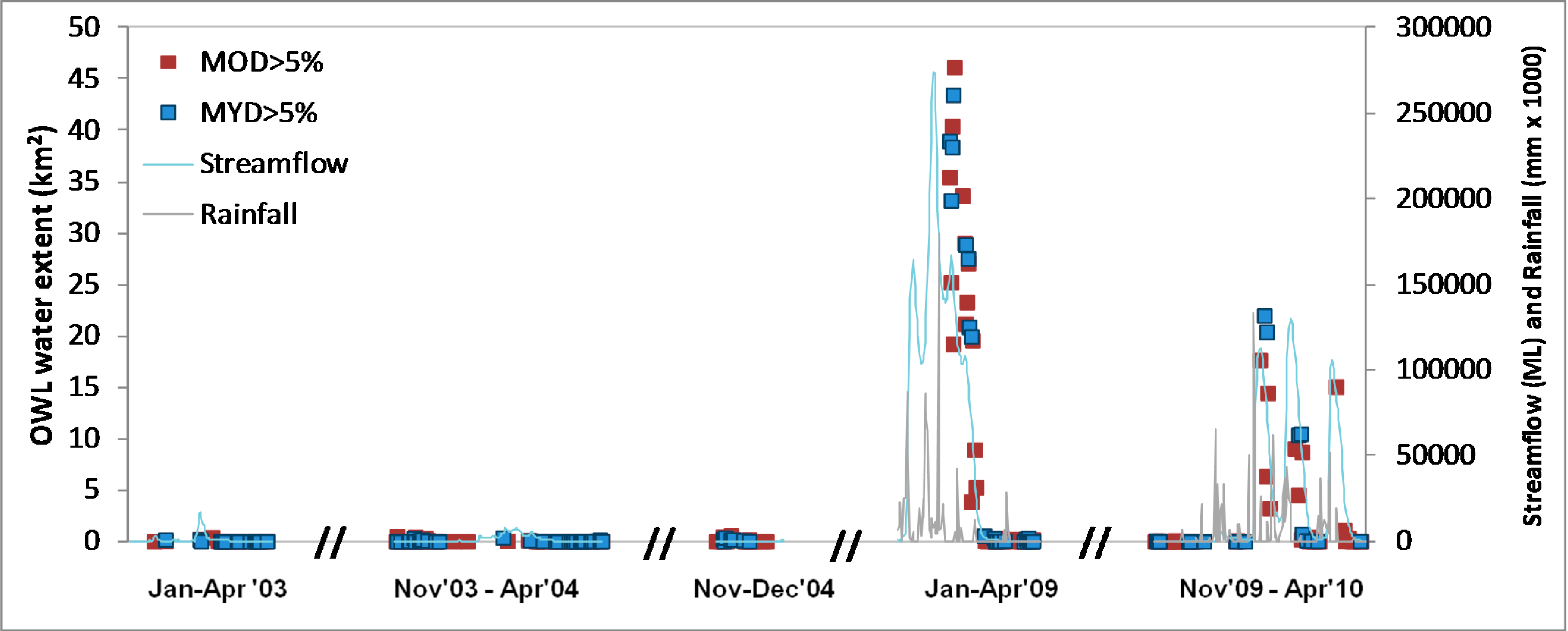
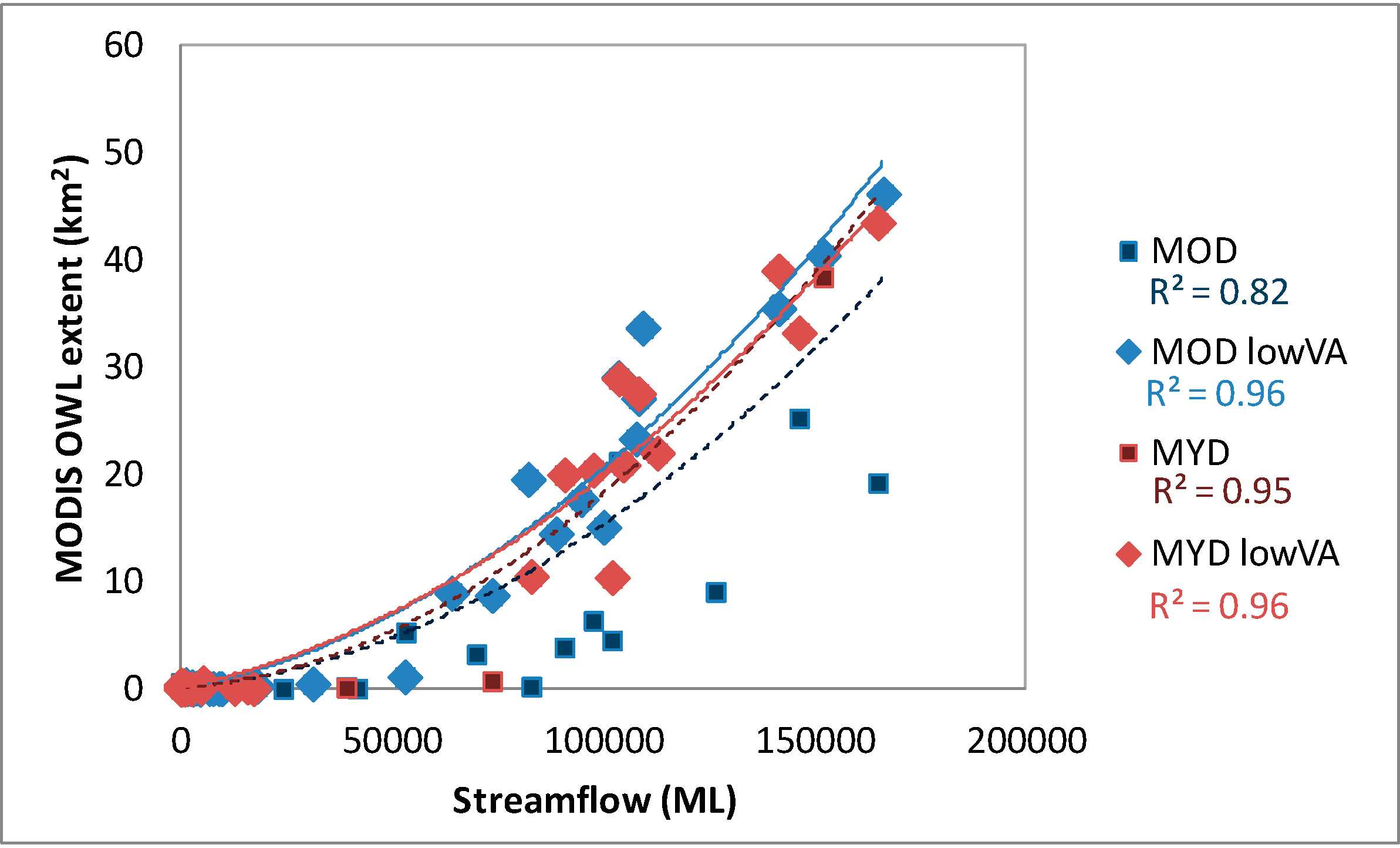
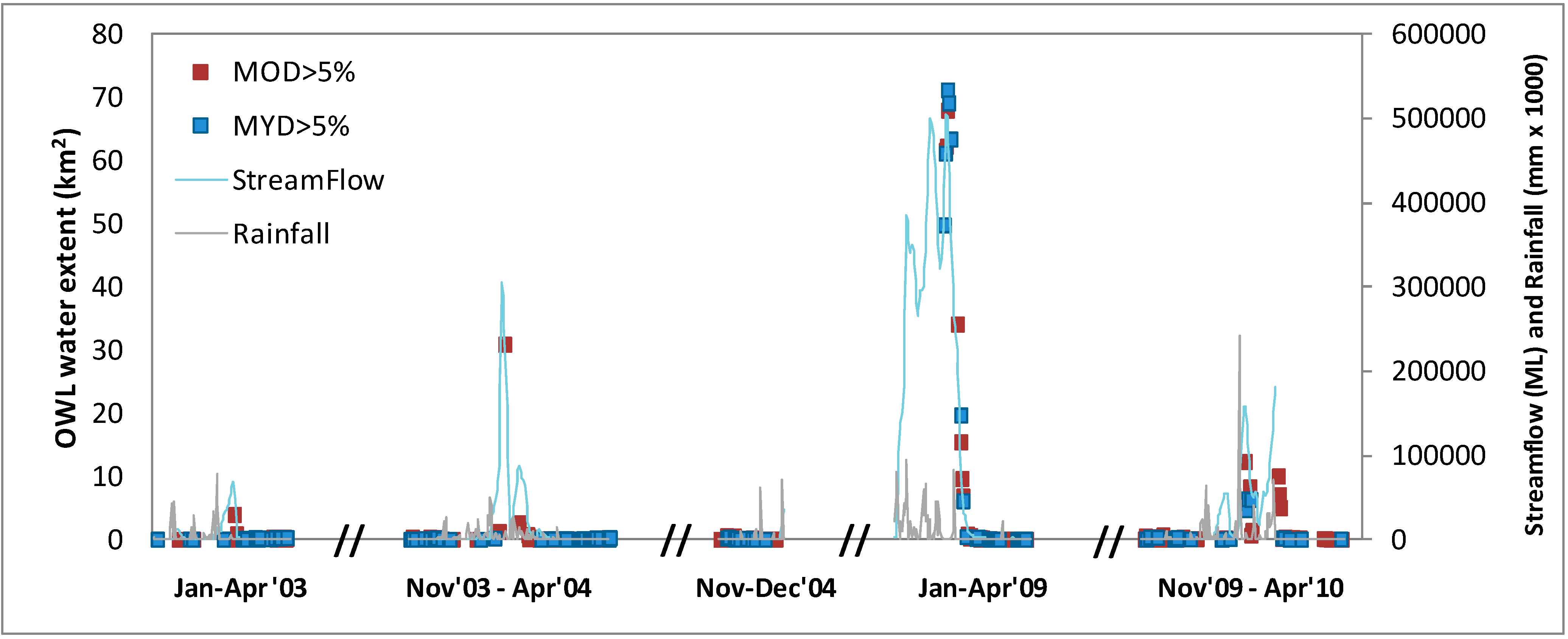
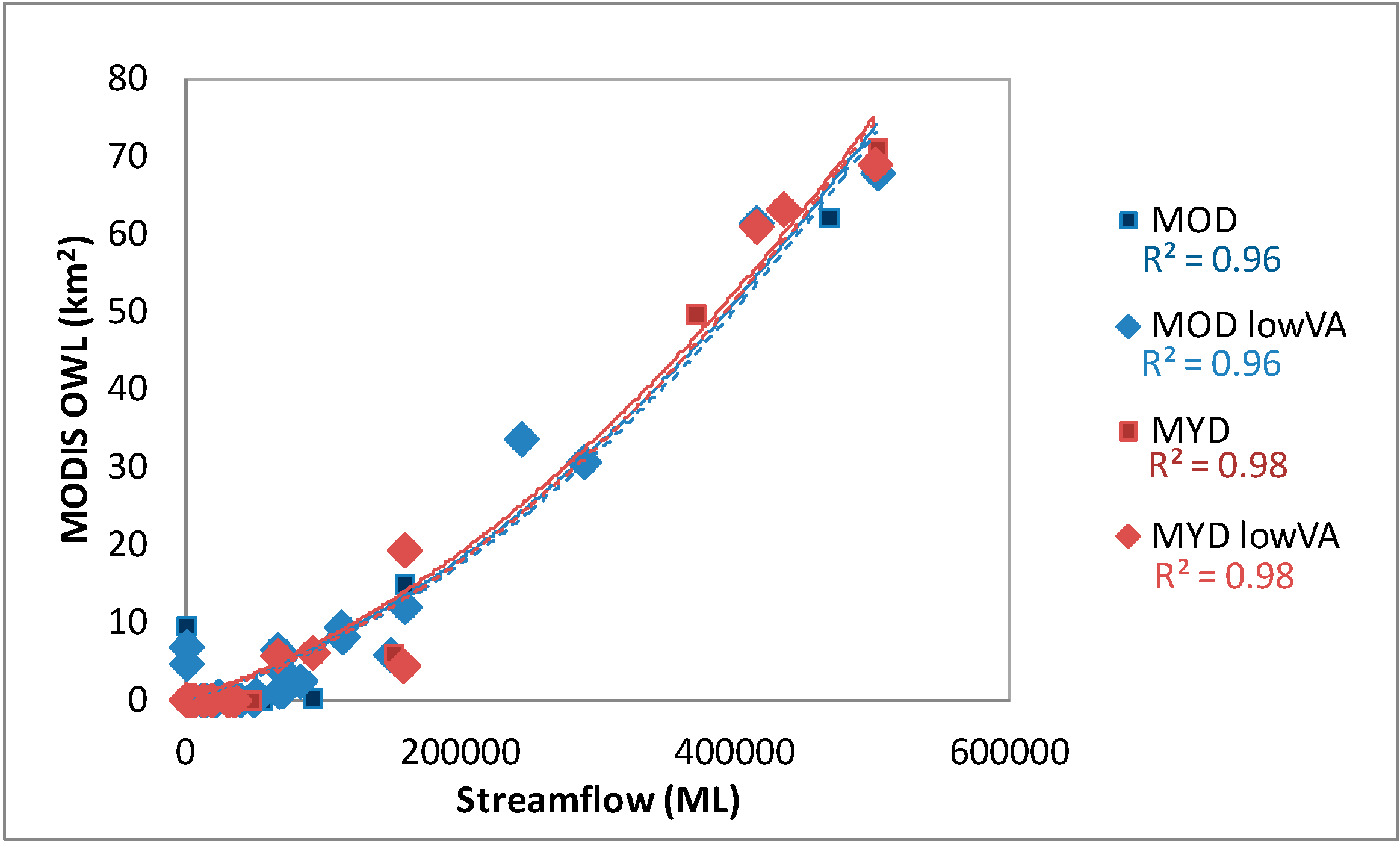
5.2. Relationship between MODIS OWL, Streamflow and Rainfall Data
5.2.1. Sites not Expected to Flood (D1 and D2)


| Data | OWL Threshold (%) | |||||||||||||||
|---|---|---|---|---|---|---|---|---|---|---|---|---|---|---|---|---|
| 1 | 2 | 3 | 4 | 5 | 6 | 7 | 8 | 9 | 10 | 11 | 12 | 13 | 14 | 15 | 16 | |
| MOD—D1 | 2779 | 50 | 9 | 2 | 2 | 1 | 0 | 0 | 0 | 3 | 0 | 0 | 0 | 0 | 0 | 0 |
| MYD—D1 | 1862 | 46 | 7 | 0 | 1 | 0 | 0 | 0 | 0 | 1 | 0 | 0 | 0 | 0 | 1 | 0 |
| MOD—D2 | 4623 | 1058 | 380 | 101 | 18 | 0 | 0 | 0 | 0 | 0 | 0 | 0 | 0 | 0 | 0 | 0 |
| MYD—D2 | 2235 | 618 | 368 | 164 | 52 | 0 | 0 | 0 | 0 | 0 | 0 | 0 | 0 | 0 | 0 | 0 |
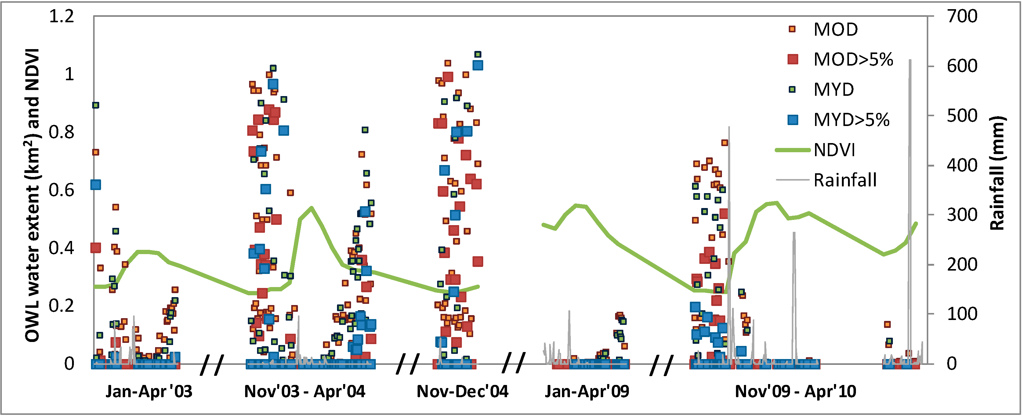
5.2.2. Sites Expected to Flood (W1 and W2)


6. Discussion
- For floods with MODIS pixels containing a high percentage of water within it, the MODIS OWL flood extent will reduce as view angle (or range distance) increases. Where possible, removing the pixels having a large view angle (or range distance greater than 1000 km) seems to improve the multi-temporal consistency.
- For MODIS pixels having a low proportion of inundation (especially for values less than 6% water) the total MODIS OWL flood extent will be larger compared to those with a low view angle. In this case, removing pixels containing less than 6% water in the MODIS OWL helps reduce commission errors (i.e., where pixels are incorrectly mapped as flooded).
- For the MODIS OWL algorithm, there is no notable difference between the MOD and MYD water maps. The main difference appears to be the reduced number of MYD scenes available due to increased cloud cover occurring in the afternoons in tropical regions.
- Soil and vegetation cover may have an influence on commission errors when the relative azimuth angle is low, as seen for Site D2 which had a spectral appearance of water according to the MODIS OWL algorithm. These same errors were not seen at Site D1 when the 6% MODIS OWL threshold was applied. The use of a flood likelihood mask could be used to eliminate areas not expected to flood. Such a mask could include height information from a DEM, to ensure only valleys and lowlands are able to be mapped as water, such as Martinis et al. [33], which would eliminate Site D2 as a potential flood zone.
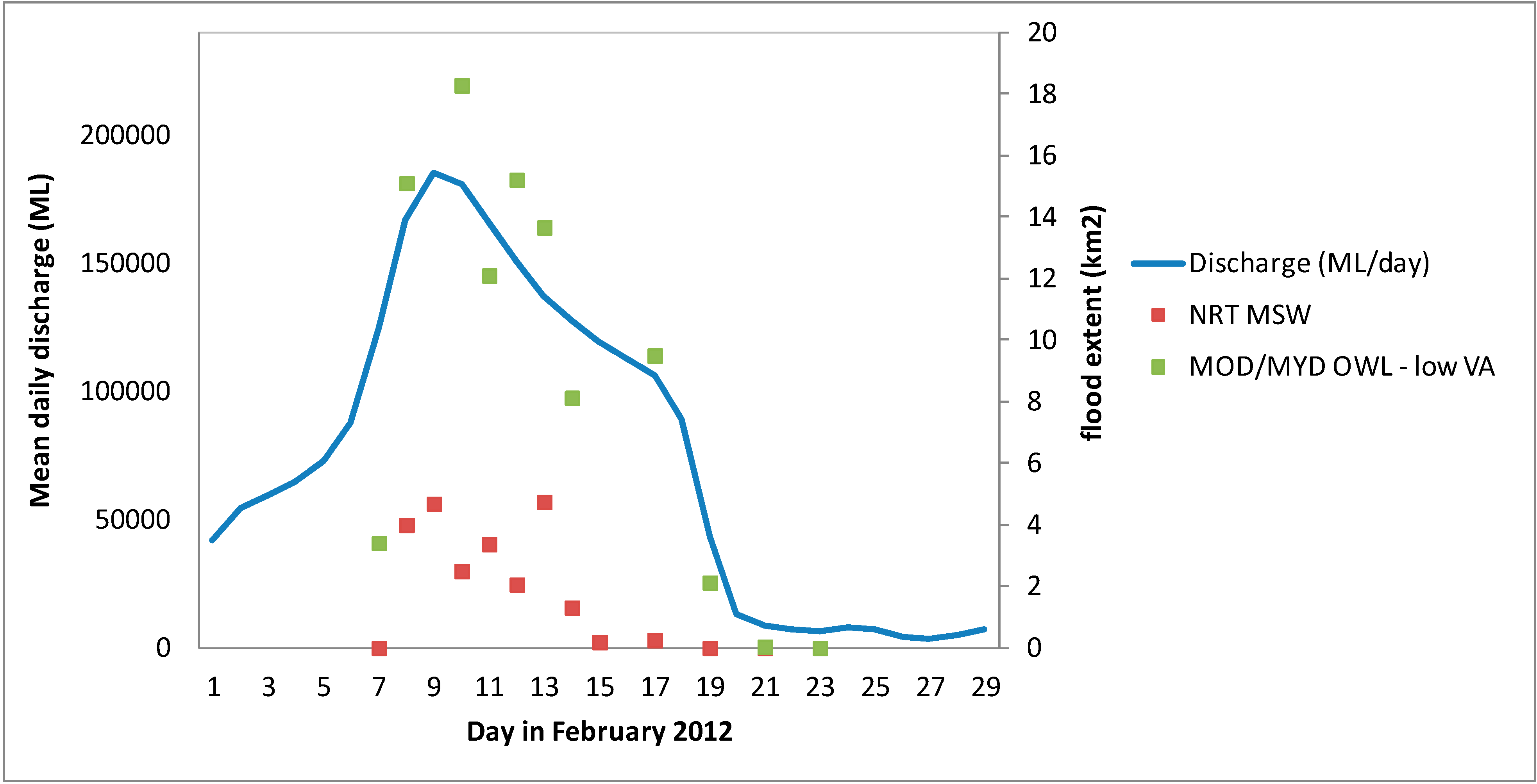
- Unfortunately remnant cloud or cloud shadow, that are not removed with the NASA generated cloud mask algorithm, cannot be automatically detected and removed. However for those pixels remaining after a flood-likelihood mask and a 6% MODIS OWL threshold is applied, a multi-temporal algorithm could be used to detect uncharacteristic spikes in flood extent. This would be a relatively simple process since the location of cloud/cloud shadow varies for each MODIS image. The NASA NRT MODIS Global Flood Map product [10] also identifies most cloud shadow as water, hence they define a pixel as wet when it has been identified as water for two of more days. For priority areas, it may be possible to develop a relationship between MODIS OWL extent and streamflow based on historical data with low view angle, and preferably good solar/viewing geometry. That way, pixels containing a large range distance could be substituted with the historical OWL extent values according to flow gauge data. However this will only work for characteristic flood events that follow historical flood patterns.
7. Conclusions and Recommendations
- Select MODIS OWL values of at least 6% water as it eliminates most commission errors.
- In some cases it may be necessary to exclude pixels having a low relative azimuth angle (i.e., the angle between the MODIS’ and sun’s azimuth angles) as this introduces commission errors in some spectrally dark pixels. However, a flood likelihood mask will also reduce the number of spectrally dark pixels which may be confused with water.
- Use daily MODIS OWL data of low view angle (range distance less than 1000 km) where possible.
- In some situations, data may be limited and all cloud-free dates are needed regardless of range distance and solar/viewing geometry. In this case, temporal averaging could be used to reduce the daily fluctuations in flood extent and to identify outliers.
Acknowledgments
Author Contributions
Conflicts of Interest
References
- Ryu, J.-H.; Won, J.-S.; Min, K.D. Waterline extraction from Landsat TM data in a tidal flat. A case study in Gomso Bay, Korea. Remote Sens. Environ. 2002, 83, 442–456. [Google Scholar] [CrossRef]
- Frazier, P.S.; Page, K.J. Water body detection and delineation with Landsat TM data. Photogramm. Eng. Remote Sens. 2000, 66, 1461–1467. [Google Scholar]
- Ward, D.P.; Hamilton, S.K.; Jardine, T.D.; Pettit, N.E.; Tews, E.K.; Olley, J.M.; Bunn, S.E. Assessing the seasonal dynamics of inundation, turbidity, and aquatic vegetation in the Australian wet-dry tropics using optical remote sensing. Ecohydrology 2013, 6, 312–323. [Google Scholar] [CrossRef]
- Gao, B.C. NDWI—A normalized difference water index for remote sensing of vegetation liquid water from space. Remote Sens. Environ. 1996, 58, 257–266. [Google Scholar] [CrossRef]
- Xu, H. Modification of normalised difference water index (NDWI) to enhance open water features in remotely sensed imagery. Int. J. Remote Sens. 2006, 27, 3025–3033. [Google Scholar] [CrossRef]
- McFeeters, S.K. The use of normalized difference water index (NDWI) in the delineation of open water features. Int. J. Remote Sens. 1996, 17, 1425–1432. [Google Scholar] [CrossRef]
- Dartmouth Flood Observatory. Available online: http://floodobservatory.colorado.edu (accessed on 19 November 2014).
- Brakenridge, R.; Anderson, E. MODIS-based flood detection, mapping and measurement: The potential for operational hydrological applications. In Transboundary Floods: Reducing Risks through Flood Management; Marsalek, J., Stancalie, G., Balint, G., Eds.; Springer Netherlands: Berlin, Germany, 2006; pp. 1–12. [Google Scholar]
- De Groeve, T.; Vernaccini, L.; Brakenridge, G.R.; Adler, R.; Ricko, M.; Wu, H.; Thielen, J.; Salamon, P.; Policelli, F.S.; Slayback, D.; et al. Global Integrated Flood Map. A JRC Technical Report, 2012; Publications Office of the European Union: Luxembourg, European Union, 2013. [Google Scholar]
- NASA. NRT Global Flood Mapping. Available online: oas.gsfc.nasa.gov (accessed on 31 October 2014).
- Weiss, D.J.; Crabtree, R.L. Percent surface water estimation for MODIS BRDF 16-day image composites. Remote Sens. Environ. 2011, 115, 2035–2046. [Google Scholar] [CrossRef]
- Guerschman, J.P.; Warren, G.; Byrne, G.; Lymburner, L.; Mueller, N.; Van-Dijk, A. MODIS-Based Standing Water Detection for Flood and Large Reservoir Mapping: Algorithm Development and Applications for the Australian Continent; CSIRO: Canberra, Australia, 2011. [Google Scholar]
- Kwak, Y.; Park, J.; Fukami, K. Estimating floodwater from MODIS time series and SRTM DEM data. Artif. Life Robot. 2014, 19, 95–102. [Google Scholar] [CrossRef]
- Ordoyne, C.; Friedl, M.A. Using MODIS data to characterize seasonal inundation patterns in the Florida Everglades. Remote Sens. Environ. 2008, 112, 4107–4119. [Google Scholar] [CrossRef]
- Chen, Y.; Cuddy, S.M.; Wang, B.; Merrin, L.E.; Pollock, D.; Sims, N. Linking inundation timing and extent to ecological response models using the Murray-Darling Basin Floodplain Inundation Model (MDB-FIM). In Proceedings of MODSIM2011: The 19th International Congress on Modelling and Simulation, Perth, Australia, 12–16 December 2011.
- Huang, C.; Chen, Y.; Wu, J. Mapping spatio-temporal flood inundation dynamics at large river basin scale using time-series flow data and MODIS imagery. Int. J. Appl. Earth Obs. Geoinf. 2014, 26, 350–362. [Google Scholar] [CrossRef]
- Huang, C.; Chen, Y.; Wu, J.; Yu, J. Detecting floodplain inundation frequency using MODIS time-series imagery. In Proceedings of Agro-Geoinformatics2012: The 1st International Conference on Agro-Geoinformatics, Shanghai, China, 2–4 August 2012.
- Huang, S.; Li, J.; Xu, M. Water surface variations monitoring and flood hazard analysis in Donting Lake area using long-term Terra/MODIS data time series. Natural Hazards 2012, 62, 93–100. [Google Scholar] [CrossRef]
- Chen, Y.; Huang, C.; Ticehurst, C.; Merrin, L.; Thew, P. An evaluation of MODIS daily and 8‑day composite products for floodplain and wetland inundation mapping. Wetlands 2013, 33, 823–835. [Google Scholar] [CrossRef]
- Doble, R.; Crosbie, R.; Peeters, L.; Joehnk, K.; Ticehurst, C. Modelling overbank flood recharge at a continential scale. Hydrol. Earth Syst. Sci. 2014, 18, 1273–1288. [Google Scholar] [CrossRef]
- Karim, F.; Petheram, C.; Marvanek, S.; Ticehurst, C.; Wallace, J.; Gouweleeuw, B. The use of hydrodynamic modelling and remote sensing to estimate floodplain inundation and flood discharge in a large tropical catchment. In Proceedings of MODSIM2011: The 19th International Congress on Modelling and Simulation, Perth, Australia, 12–16 December 2011.
- Ticehurst, C.J.; Chen, Y.; Karim, F.; Dutta, D.; Gouweleeuw, B. Using MODIS for mapping flood events for use in hydrological and hydrodynamic models: Experiences so far. In Proceedings of MODSIM2013, 20th International Congress on Modelling and Simulation, Adelaide, Australia, 1–6 December 2013.
- MDBA (Murray-Darling Basin Authority). Chowilla Floodplain. Environmental Water Management Plan. Available online: www.mdba.gov.au/sites/default/files/pubs/CFSL_FA_screen.pdf (accessed on 27 February 2012).
- Dutta, D.; Karim, F.; Ticehurst, C.; Marvanek, S.; Petheram, C. Floodplain Inundation Mapping and Modelling in the Flinders and Gilbert Catchments. A Technical Report to the Australian Government from the CSIRO Flinders and Gilbert Agricultural Resource Assessment, Part of the North Queensland Irrigated Agriculture Strategy; CSIRO Water for a Healthy Country and Sustainable Agriculture Flagships: Canberra, Australia, 2013. [Google Scholar]
- Royal Geographical Society of Queensland. Queensland by Degrees. Available online: www.rgsq.org.au/qldbydeg (accessed on 30 April 2014).
- Bartley, R.; Thomas, M.F.; Clifford, D.; Phillip, S.; Brough, D.; Harms, D.; Willis, R.; Gregory, L.; Glover, M.; Moodie, K.; et al. Land Suitability: Technical Methods. A Technical Report to the Australian Government for the Flinders and Gilbert Agricultural Resource Assessment (FGARA) Project; CSIRO: Canberra, Australia, 2013. [Google Scholar]
- NASA. Reverb|Echo—The Next Generation Earth Science Discovery Tool. Available online: reverb.echo.nasa.gov/reverb (accessed on 19 November 2014).
- Vermote, E.; Kitchenova, S. MOD09 (Surface Reflectance) User’s Guide. Available online: modis-sr.ltdri.org (accessed on 1 May 2014).
- Hu, C. A novel ocean color index to detect floating algae in the global oceans. Remote Sens. Environ. 2009, 113, 2118–2129. [Google Scholar] [CrossRef]
- Feng, L.; Hu, C.; Chen, X.; Cai, X.; Tian, L.; Gan, W. Assessment of inundation changes of Poyang Lake using MODIS observations between 2000 and 2010. Remote Sens. Environ. 2012, 121, 80–92. [Google Scholar] [CrossRef]
- Xin, Q.; Woodcock, C.E.; Liu, J.; Tan, B.; Melloh, R.A.; Davis, R.E. View angle effects on MODIS slow mapping in forests. Remote Sens. Environ. 2012, 118, 50–59. [Google Scholar] [CrossRef]
- Chen, Y.; Wang, B.; Pollino, C.A.; Cuddy, S.M.; Merrin, L.E.; Huang, C. Estimate of flood inundation and retention on wetlands using remote sensing and GIS. Ecohydrology 2014, 7, 1412–1420. [Google Scholar]
- Martinis, S.; Twele, A.; Strobl, C.; Kersten, J.; Stein, E. A multi-scale flood monitoring system based on fully automatic MODIS and TerraSAR-X processing chains. Remote Sens. 2013, 5, 5598–5619. [Google Scholar] [CrossRef]
© 2014 by the authors; licensee MDPI, Basel, Switzerland. This article is an open access article distributed under the terms and conditions of the Creative Commons Attribution license (http://creativecommons.org/licenses/by/4.0/).
Share and Cite
Ticehurst, C.; Guerschman, J.P.; Chen, Y. The Strengths and Limitations in Using the Daily MODIS Open Water Likelihood Algorithm for Identifying Flood Events. Remote Sens. 2014, 6, 11791-11809. https://doi.org/10.3390/rs61211791
Ticehurst C, Guerschman JP, Chen Y. The Strengths and Limitations in Using the Daily MODIS Open Water Likelihood Algorithm for Identifying Flood Events. Remote Sensing. 2014; 6(12):11791-11809. https://doi.org/10.3390/rs61211791
Chicago/Turabian StyleTicehurst, Catherine, Juan Pablo Guerschman, and Yun Chen. 2014. "The Strengths and Limitations in Using the Daily MODIS Open Water Likelihood Algorithm for Identifying Flood Events" Remote Sensing 6, no. 12: 11791-11809. https://doi.org/10.3390/rs61211791