On the Downscaling of Actual Evapotranspiration Maps Based on Combination of MODIS and Landsat-Based Actual Evapotranspiration Estimates

 ,
,
Abstract
:
1. Introduction
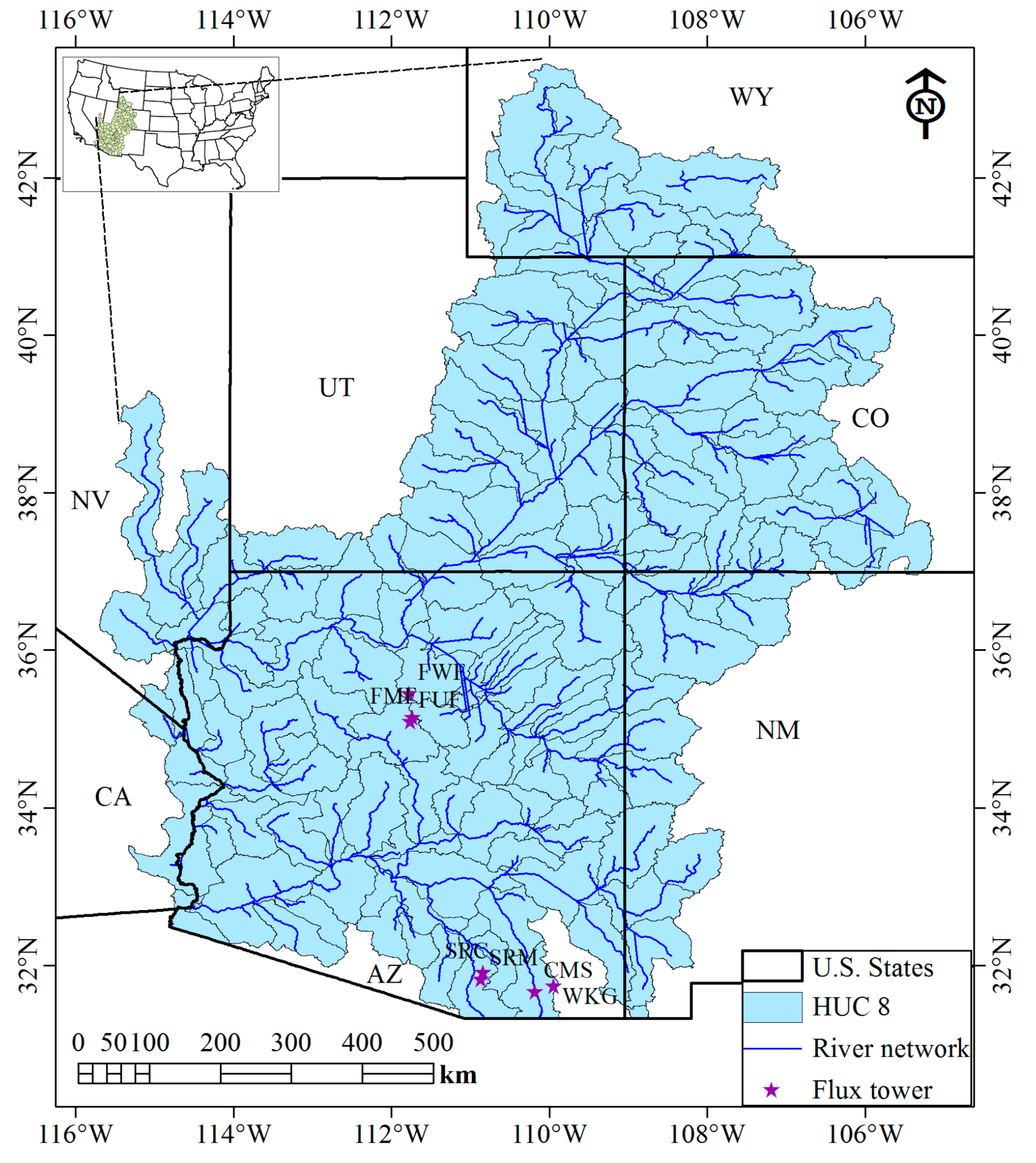
2. Study Area
3. Method
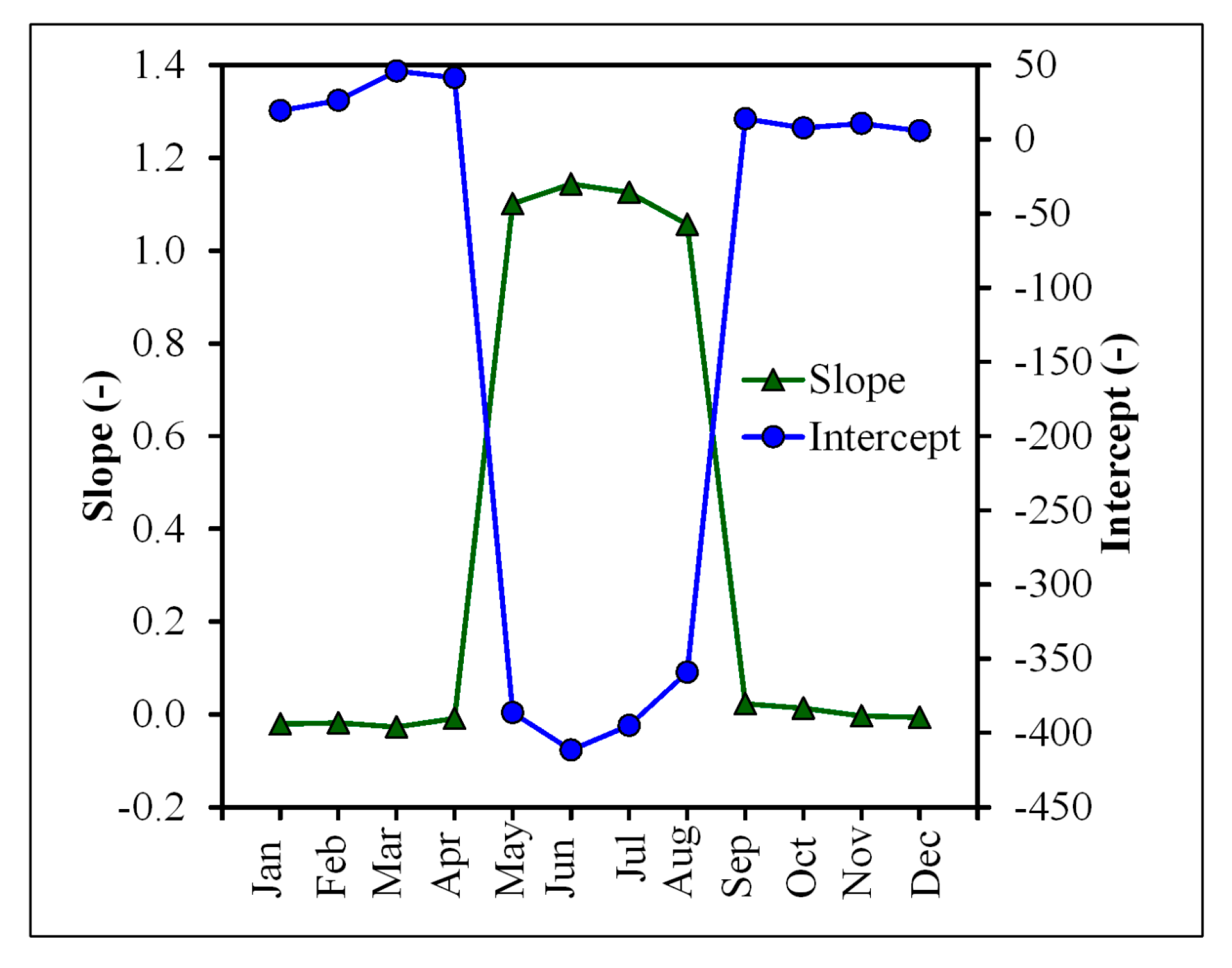
3.1. Regression (Slope-Intercept) Method

3.2. Linear with Zero Intercept (LinZI) Method
4. Data
4.1. Landsat Data
4.2. MODIS Data
4.3. Gridded FLUXNET Data
5. Evaluation of Downscaled Products
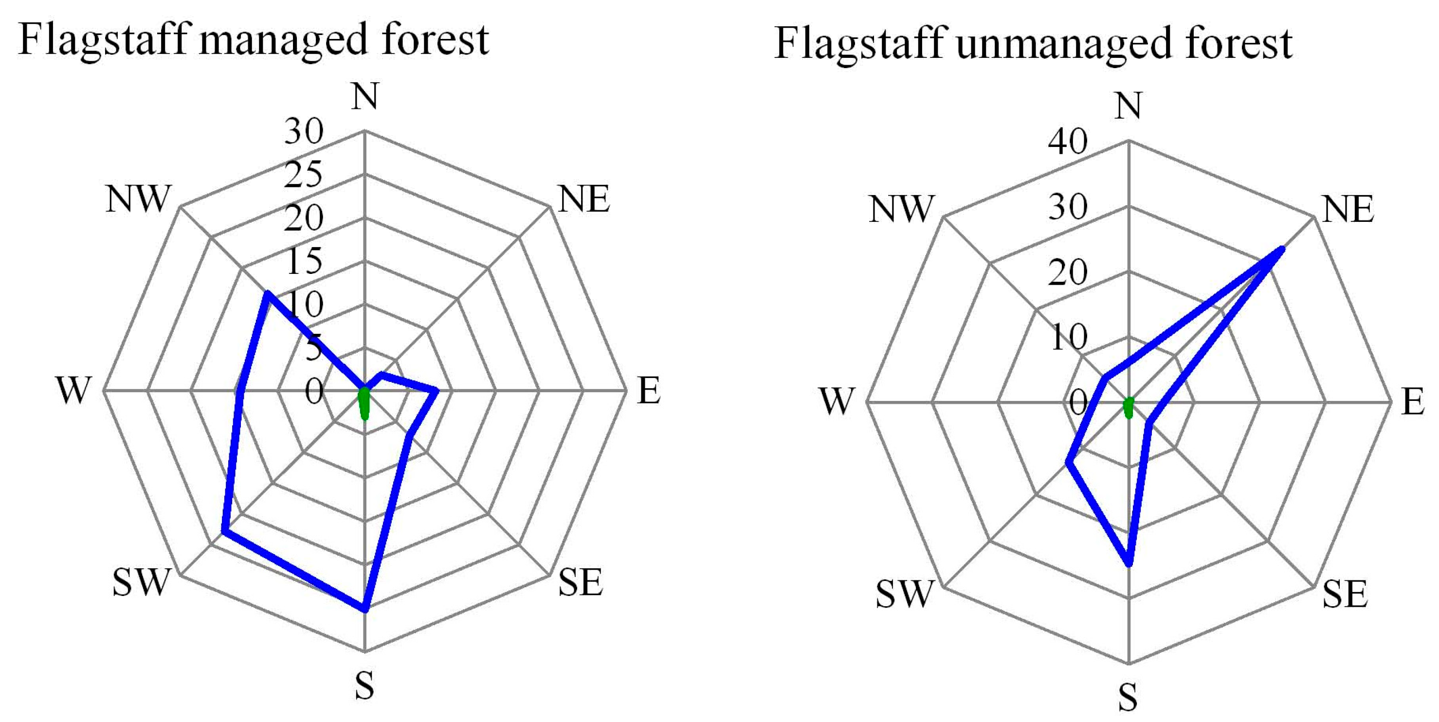
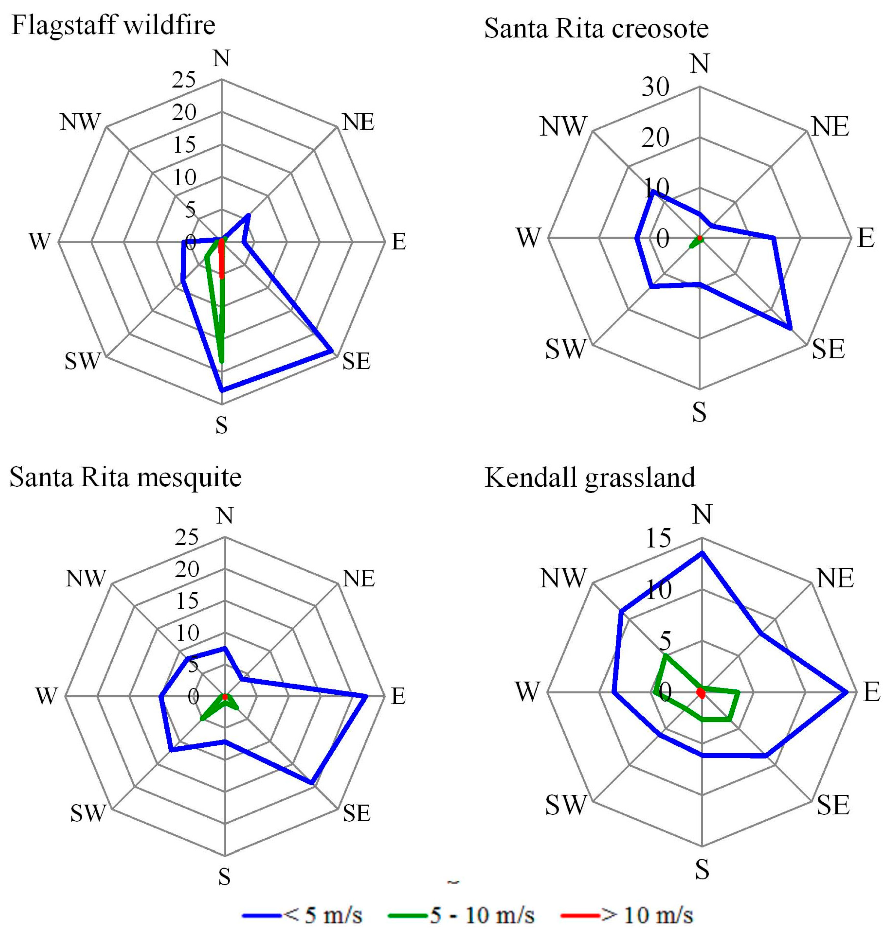
5.1. Validation Using Eddy Covariance Flux Towers

| Sl. No. | Site | Latitude (°) | Longitude (°) | Elevation (m) | Tower Height (m) | Land Cover | Landsat Path/Row | No. of Cloud-Free Images | Reference |
|---|---|---|---|---|---|---|---|---|---|
| 1 | Flagstaff managed forest | 35.1426 | −111.7273 | 2160 | 23 | Ponderosa pine forest | 37/36 | 6 | Dore et al. (2012) [52] |
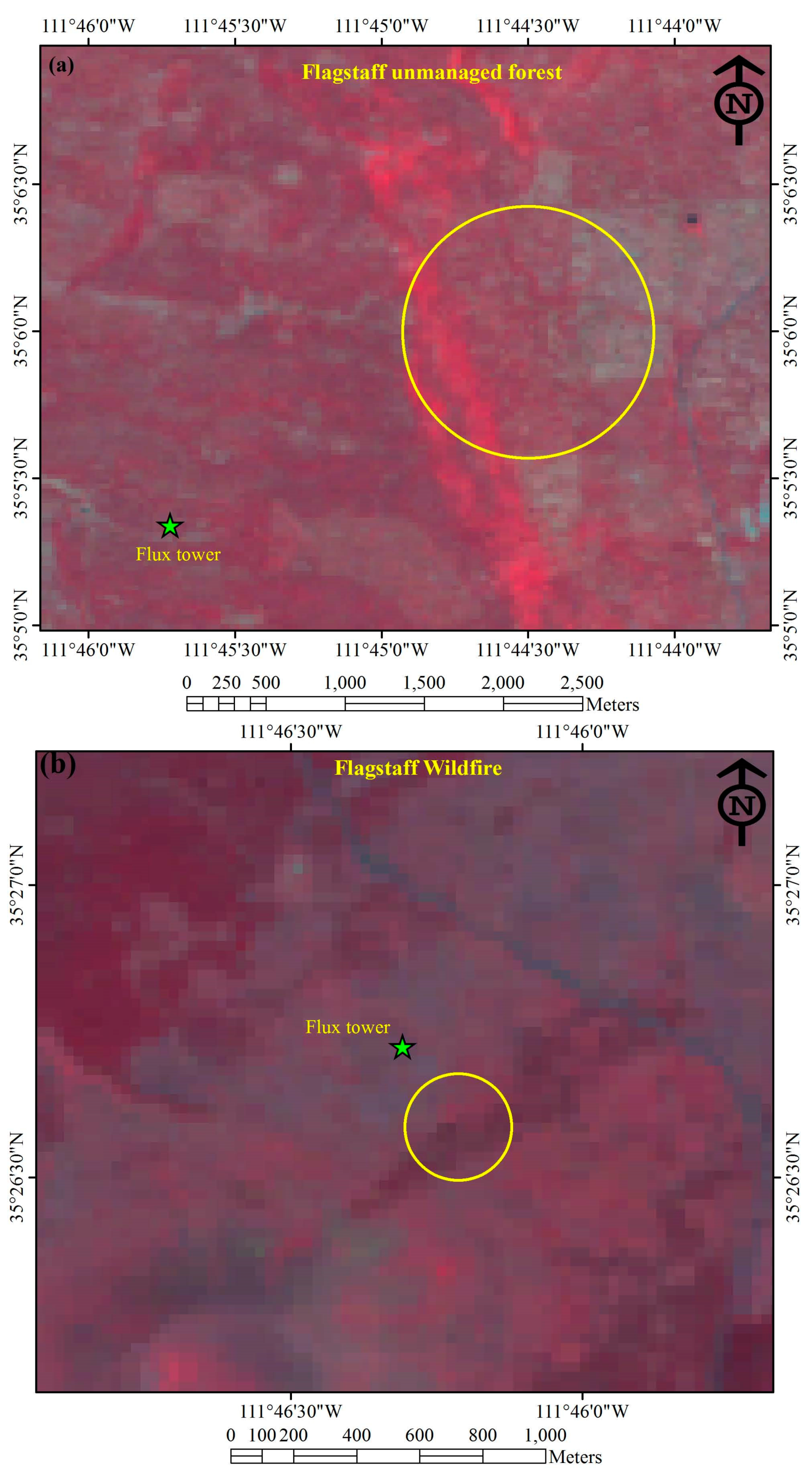
| 2 | Flagstaff unmanaged forest | 35.089 | −111.762 | 2180 | 23 | Ponderosa pine forest | 37/36 | 6 | Dore et al. (2012) [52] |
| 3 | Flagstaff wildfire | 35.4454 | −111.7718 | 2270 | 4 | Ponderosa pine forest | 37/35 | 7 | Dore et al. (2012) [52] |
| 4 | Santa Rita Creosote | 31.9083 | −110.8395 | 991 | 4.25 | Open shrub land | 36/38 | 9 | Kurc and Benton (2010) [ 53] |
| 5 | Santa Rita Mesquite | 31.8214 | −110.8661 | 1120 | 6.4 | Woody Savannas | 36/38 | 9 | Scott et al. (2009) [54] |
| 6 | Kendall Grassland | 31.7365 | −109.9419 | 1531 | 6.4 | Grassland | 35/38 | 7 | Scott et al. (2010) [55] |
| 7 | Charleston Mesquite | 31.6637 | −110.1776 | 1200 | 14 | Riparian woodland | 35/38 | 7 | Scott et al. (2004) [56] |
5.2. Evaluation Using Gridded FLUXNET Data
5.3. Evaluation Using MODIS-Based AET
6. Results and Discussion
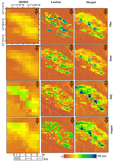
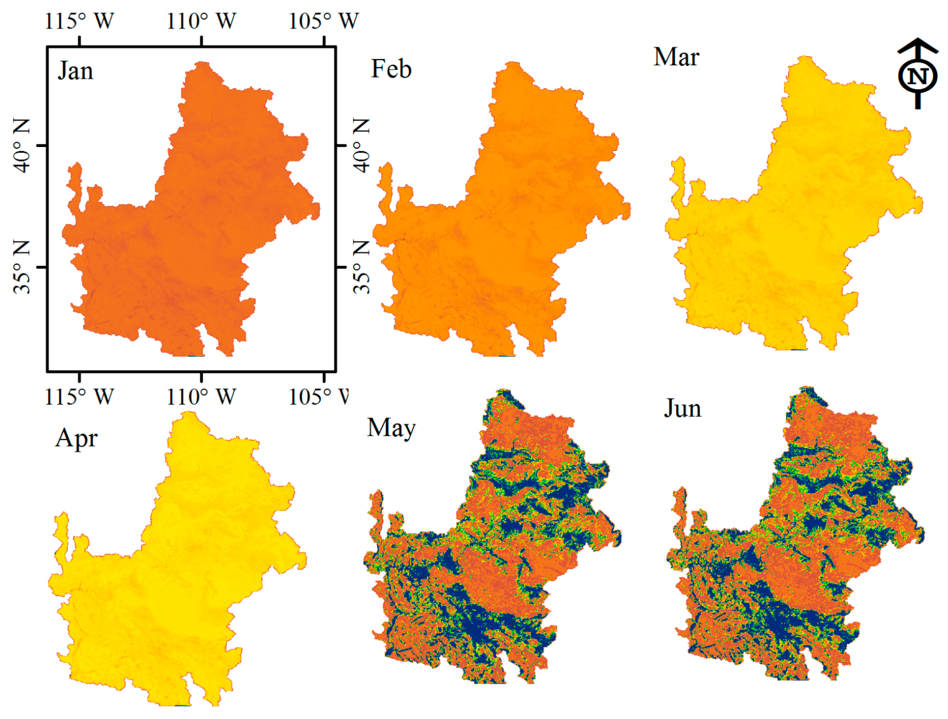
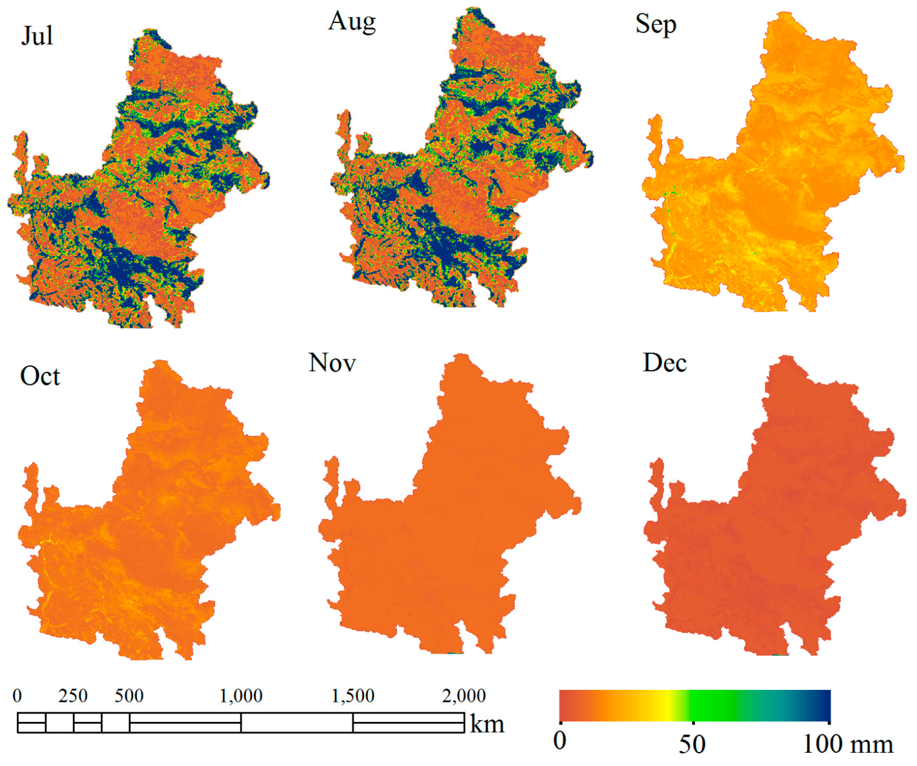
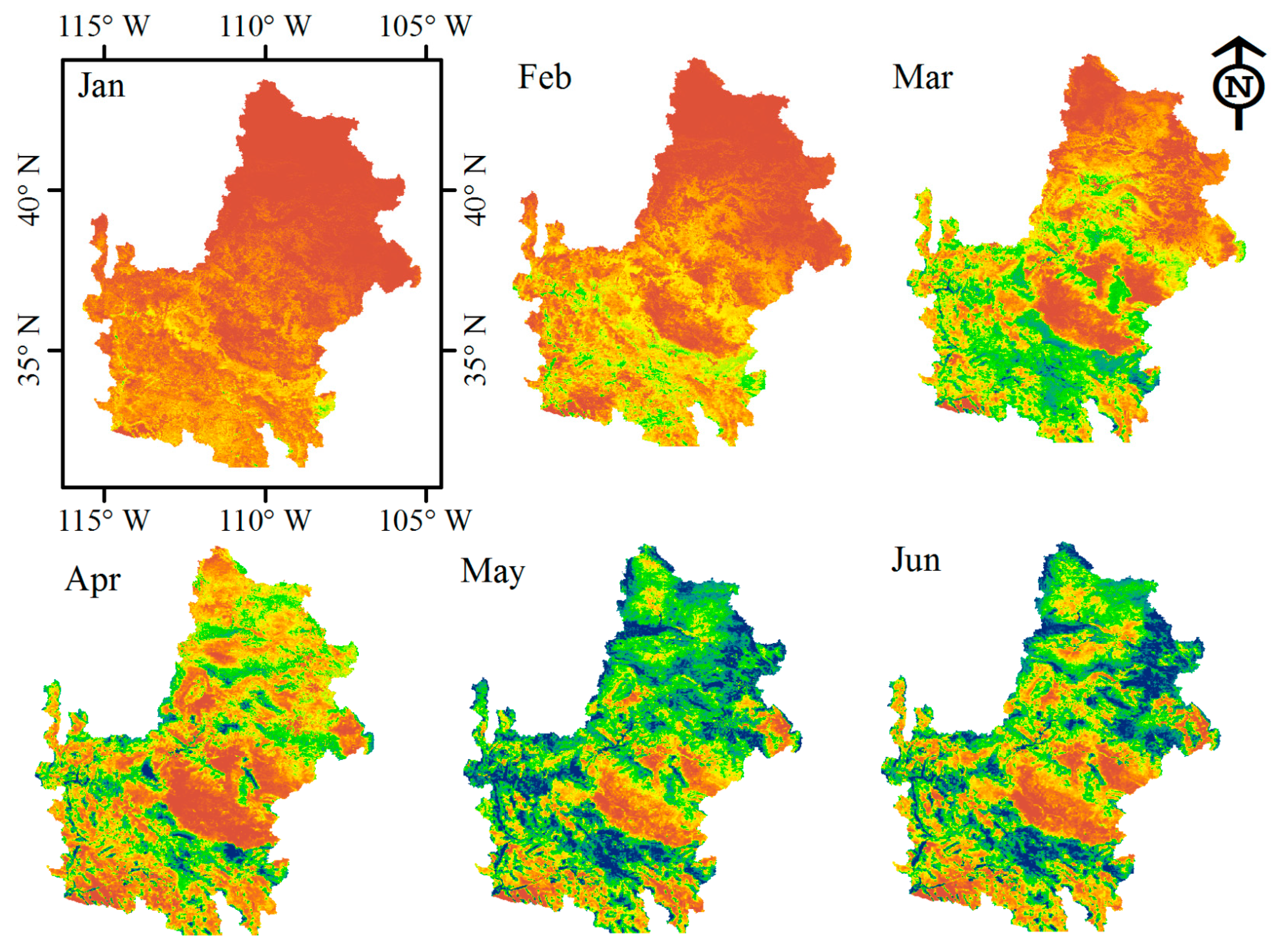
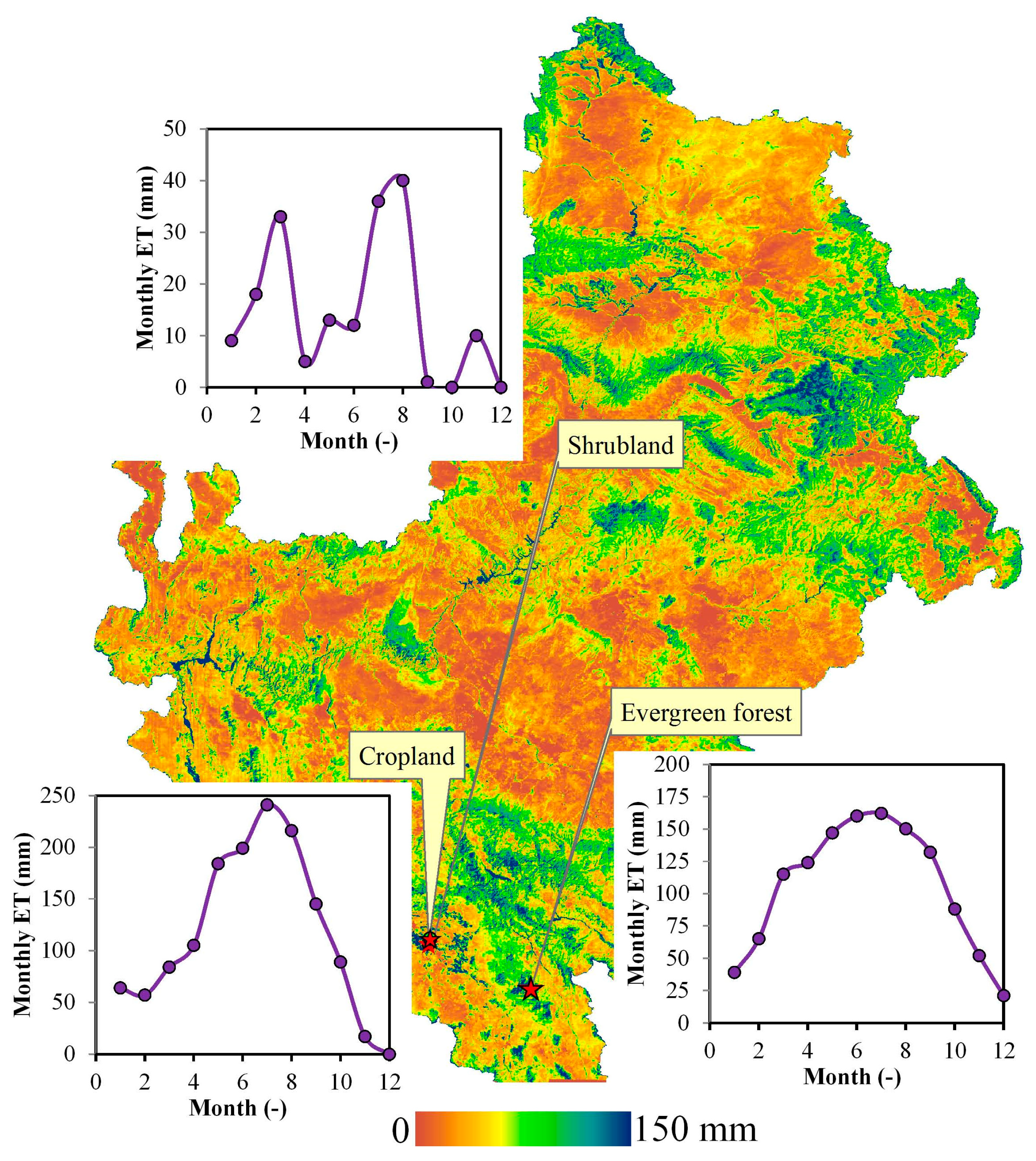
6.1. Monthly Evapotranspiration Using the Regression (Slope-Intercept) Method
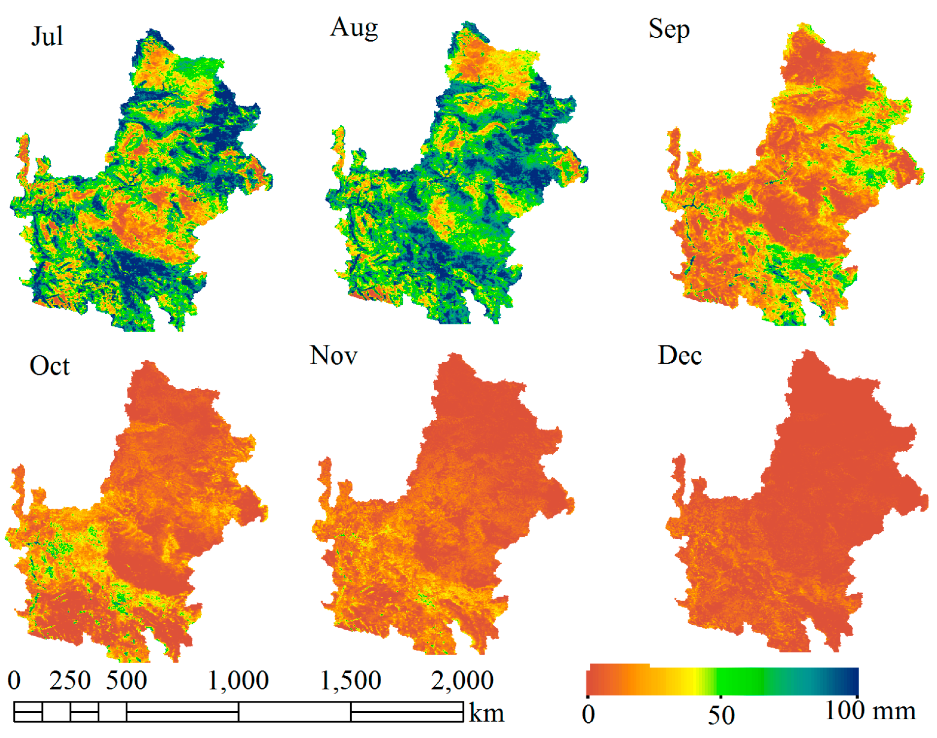
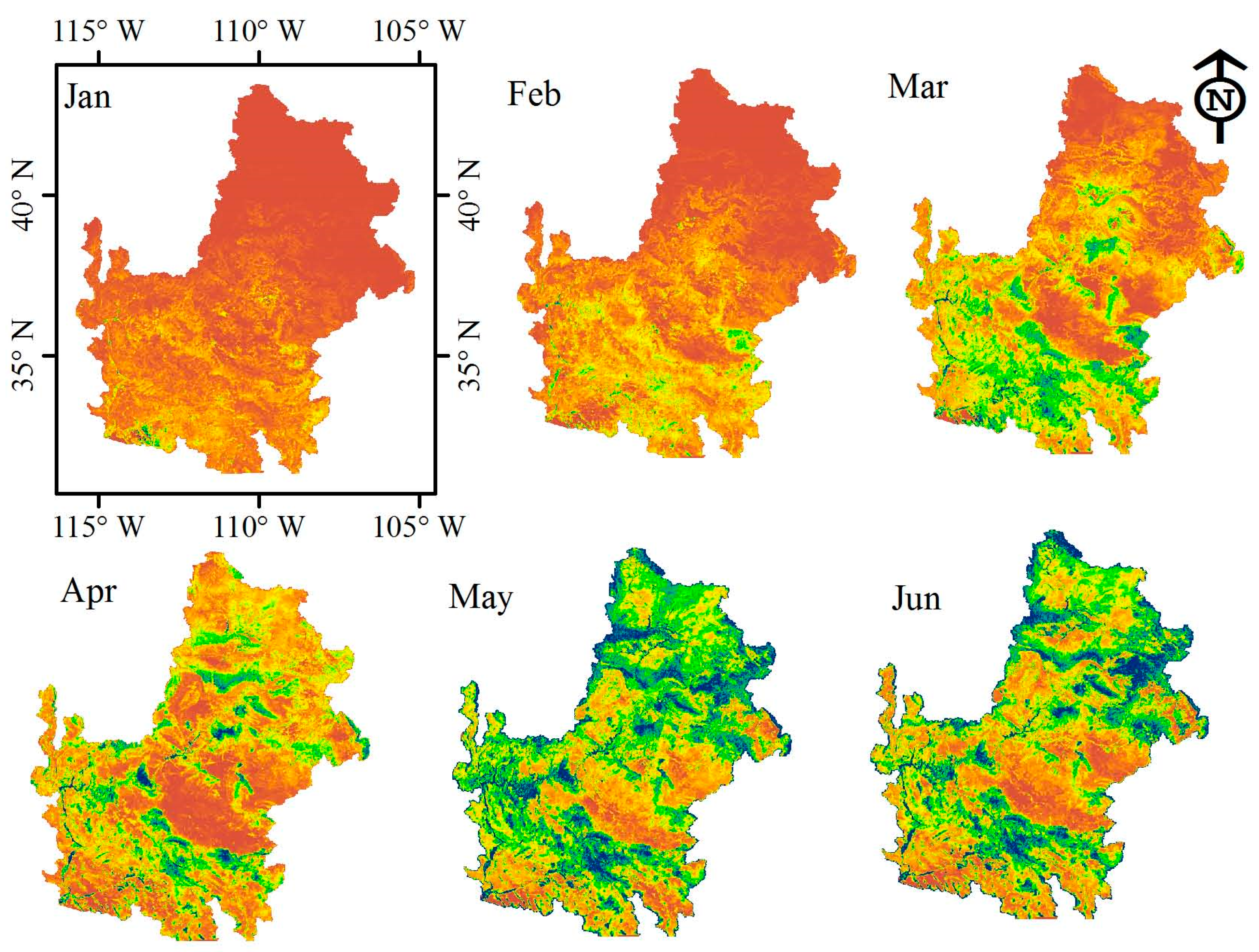
6.2. Monthly Evapotranspiration Using the LinZI Method


| Site | Mean Bias (mm) | RMSE (mm) | R2 |
|---|---|---|---|
| Flagstaff managed forest | −8 | 19 | 0.53 |
| Flagstaff unmanaged forest | 22 | 32 | 0.64 |
| Flagstaff wildfire | −16 | 22 | 0.52 |
| Santa Rita Creosote | 1 | 10 | 0.61 |
| Santa Rita Mesquite | −2 | 12 | 0.72 |
| Kendall Grassland | −9 | 13 | 0.81 |
| Charleston Mesquite | 7 | 20 | 0.88 |
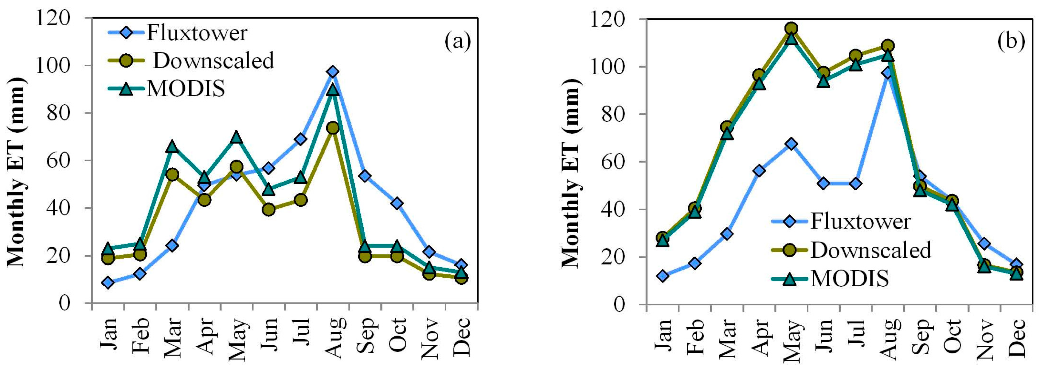
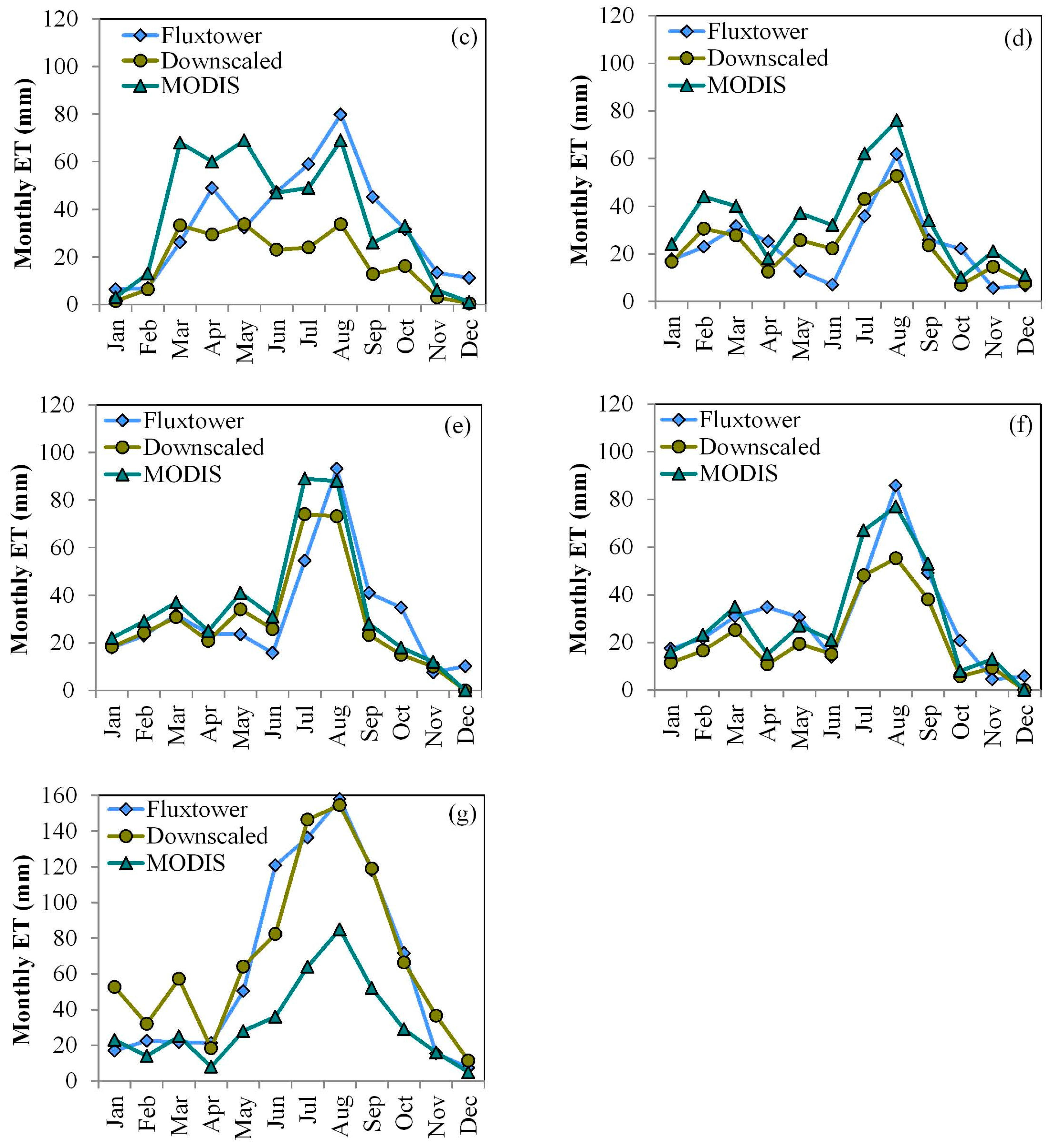
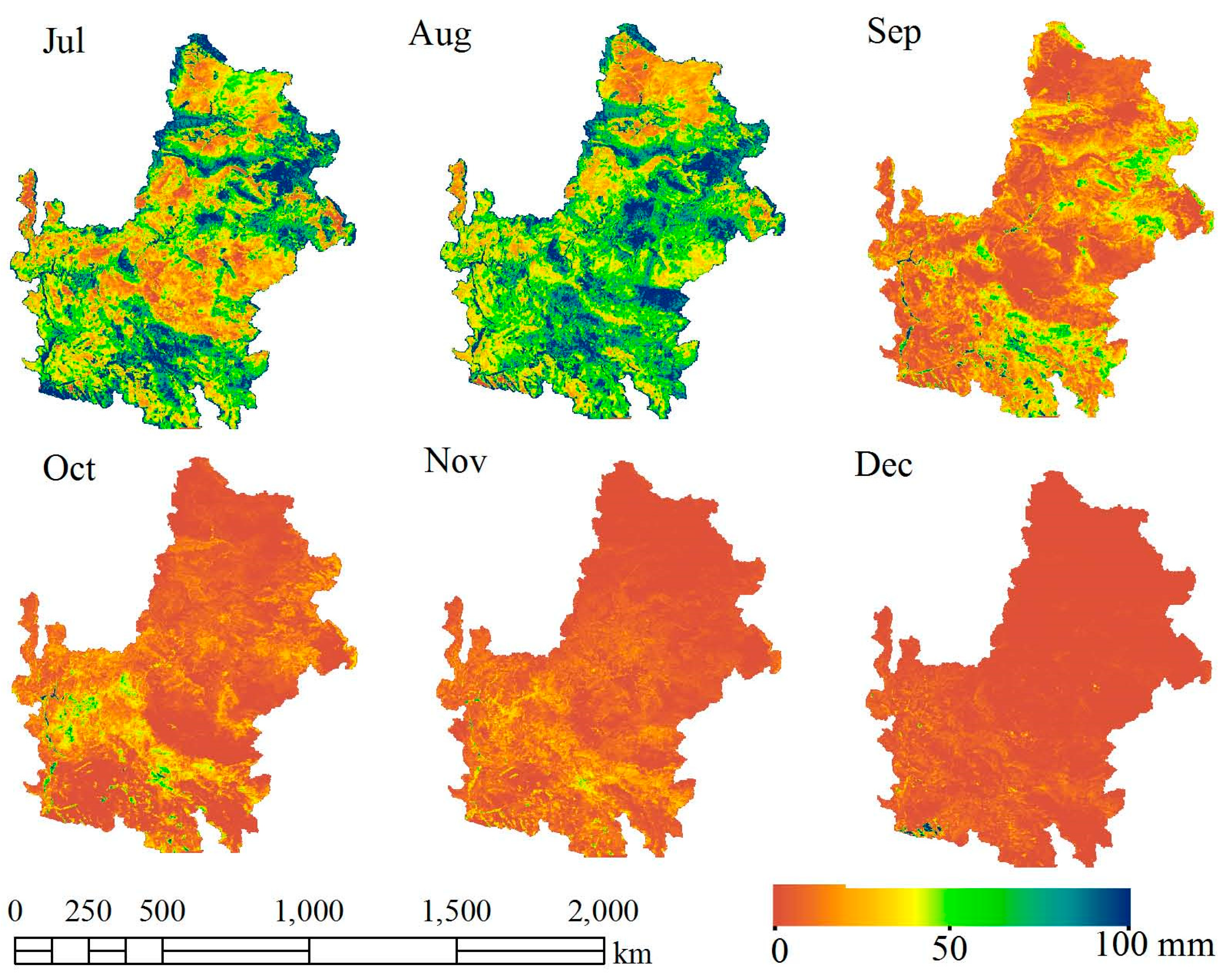
6.3. Comparison of Downscaled Monthly AET Maps with the Eddy Covariance Measurements


6.4. Comparison of Downscaled Monthly AET Maps with the Gridded FLUXNET Dataset
| Month | Slope-Intercept Method | LinZI Method | ||||
|---|---|---|---|---|---|---|
| MB (mm) | RMSE (mm) | R2 (–) | MB (mm) | RMSE (mm) | R2 (–) | |
| January | −3 | 6 | 0.01 | −4 | 6 | 0.75 |
| February | 2 | 5 | 0.01 | 0 | 8 | 0.53 |
| March | 8 | 10 | 0.08 | 4 | 12 | 0.50 |
| April | 6 | 9 | 0.05 | 1 | 9 | 0.34 |
| May | 24 | 44 | 0.14 | 18 | 22 | 0.32 |
| June | 21 | 42 | 0.13 | 10 | 17 | 0.43 |
| July | 13 | 38 | 0.19 | 7 | 20 | 0.23 |
| August | 19 | 40 | 0.24 | 20 | 26 | 0.20 |
| September | −5 | 12 | 0.15 | −8 | 12 | 0.45 |
| October | −8 | 9 | 0.25 | −10 | 12 | 0.08 |
| November | −1 | 3 | 0.02 | −4 | 6 | 0.13 |
| December | −7 | 8 | 0.01 | −9 | 9 | 0.55 |
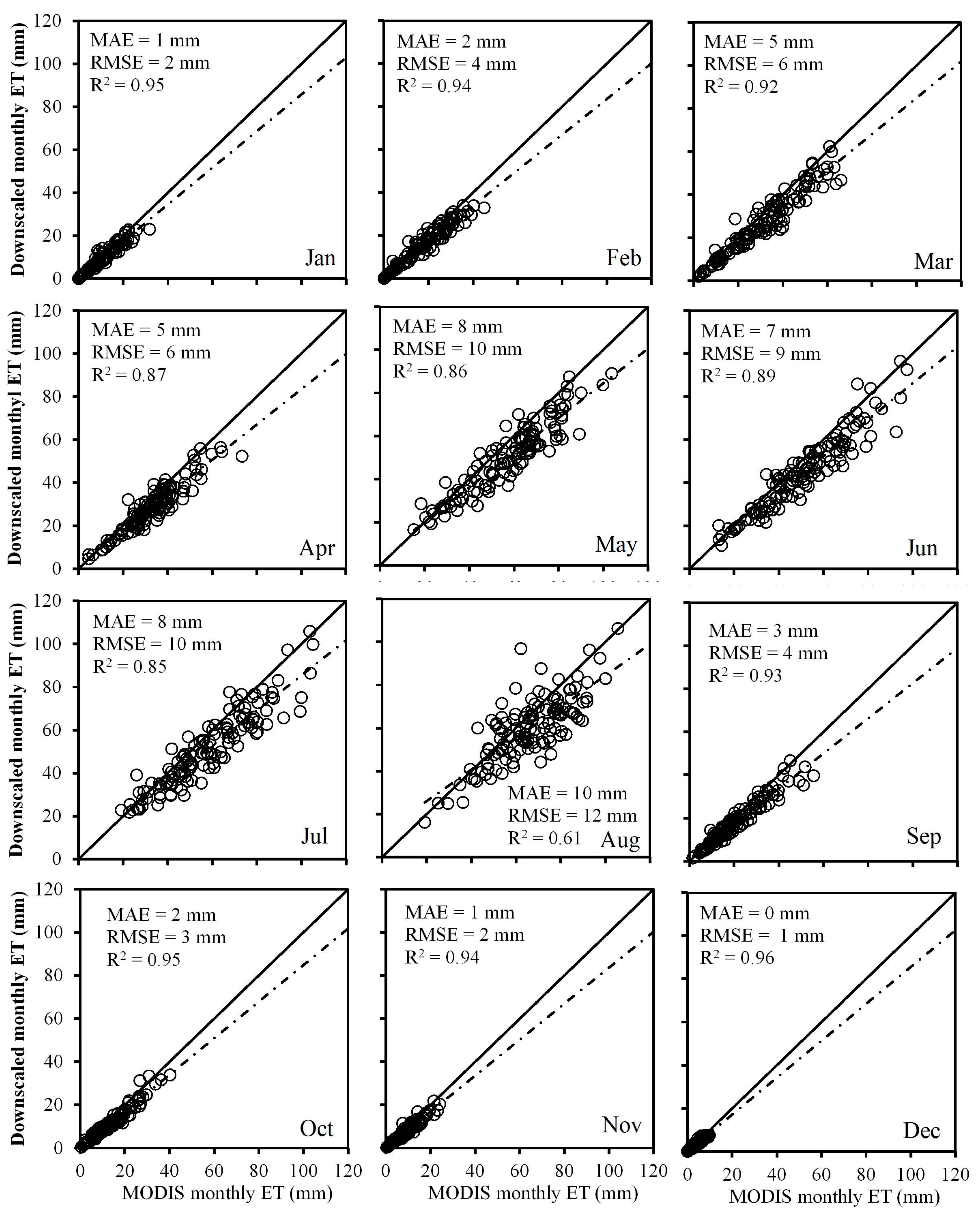
6.5. Comparison of the LinZI Method Monthly Evapotranspiration with Monthly MODIS AET Maps
7. Conclusions
Acronyms and Abbreviations
| AET | Actual evapotranspiration |
| BCM | Billion Cubic Meters |
| CMS | Charleston Mesquite |
| CRB | Colorado River Basin |
| ET | Evapotranspiration |
| ETM+ | Enhanced Thematic Mapper Plus |
| FMF | Flagstaff Managed Forest |
| FUF | Flagstaff Unmanaged Forest |
| FWF | Flagstaff Wildfire |
| HIS | Hue-Intensity-Saturation |
| HPF | High Pass Filter |
| HUC | Hydrologic Unit Code |
| IHS | Intensity-hue-saturation |
| LiDAR | Light Detection And Ranging |
| LinZI | Linear with Zero Intercept |
| LST | Land Surface Temperature |
| MAE | Mean Absolute Error |
| MB | Mean Bias |
| MODIS | Moderate Resolution Imaging Spectroradiometer |
| NASA | National Aeronautics and Space Administration |
| NLCD | National Land Cover Database |
| PALSAR | Phased Array L-band Synthetic Aperture Radar |
| PCA | Principal Component Analysis |
| RMSE | Root Mean Square Error |
| SLC | Scan Line Corrector |
| SPOT | Systeme Pour I’Observation de la Terre |
| SRC | Santa Rita Creosote |
| SRM | Santa Rita Mesquite |
| SSEBop | Operational Simplified Surface Energy Balance |
| STARFM | Spatial and Temporal Adaptive Reflectance Fusion Model |
| TM | Thematic Mapper |
| USA | United States of America |
| USGS | United States Geological Survey |
| WaterSMART | Sustain and Manage America’s Resources for Tomorrow |
| WKG | Kendall Grassland |
Acknowledgments
Author Contributions
Conflicts of Interest
References
- Chavez, P.S.; Sides, S.C.; Anderson, J.A. Comparison of three different methods to merge multiresolution and multispectral data: Landsat TM and SPOT panchromatic. Photogramm. Eng. Remote Sens. 1991, 57, 295–303. [Google Scholar]
- Long, D.; Singh, V.P. Integration of the GG model with SEBAL to produce time series of evapotranspiration of high spatial resolution at watershed scales. J. Geophys. Res.: Atmos. 2010. [Google Scholar] [CrossRef]
- McCabe, M.F.; Wood, E.F. Scale influences on the remote estimation of evapotranspiration using multiple satellite sensors. Remote Sens. Environ. 2006, 105, 271–285. [Google Scholar] [CrossRef]
- Hall, D.L.; Llinas, J. An introduction to multisensor data fusion. Proc. IEEE 1997, 85, 6–23. [Google Scholar] [CrossRef]
- Pohl, C.; van Genderen, J.L. Multisensor image fusion in remote sensing: Concepts, methods and applications. Int. J. Remote Sens. 1998, 19, 823–854. [Google Scholar] [CrossRef]
- Cliche, G.; Bonn, F.; Teillet, P. Integration of the SPOT panchromatic channel into its multispectral mode for image sharpness enhancement. Photogramm. Eng. Remote Sens. 1985, 51, 311–316. [Google Scholar]
- Carper, W.J.; Lillesand, T.M.; Kiefer, R.W. The use of intensity-hue-saturation transformations for merging SPOT panchromatic and multispectral image data. Photogramm. Eng. Remote Sens. 1990, 56, 459–467. [Google Scholar]
- Price, J.C. Combining multispectral data of differing spatial resolution. IEEE Trans. Geosci. Remote Sens. 1999, 37, 1199–1203. [Google Scholar] [CrossRef]
- Wald, L.; Ranchin, T.; Mangolini, M. Fusion of satellite images of different spatial resolutions: Assessing the quality of resulting images. Photogramm. Eng. Remote Sens. 1997, 63, 691–699. [Google Scholar]
- Karathanassi, V.; Kolokousis, P.; Ioannidou, S. A comparison study on fusion methods using evaluation indicators. Int. J. Remote Sens. 2007, 28, 2309–2341. [Google Scholar] [CrossRef]
- Garguet-Duport, B.; Girel, J.; Chassery, J.M.; Pautou, G. The use of multiresolution analysis and wavelets transform for merging SPOT panchromatic and multispectral image data. Photogramm. Eng. Remote Sens. 1996, 62, 1057–1066. [Google Scholar]
- Yocky, D.A. Multiresolution wavelet decomposition image merger of Landsat Thematic Mapper and SPOT panchromatic data. Photogramm. Eng. Remote Sens. 1996, 62, 1067–1074. [Google Scholar]
- Nunez, J.; Otazu, X.; Fors, O.; Prades, A.; Pala, V.; Arbiol, R. Multiresolution-based image fusion with additive wavelet decomposition. IEEE Trans. Geosci. Remote Sens. 1999, 37, 1204–1211. [Google Scholar] [CrossRef]
- Gao, F.; Masek, J.; Schwaller, M.; Hall, F. On the blending of the Landsat and MODIS surface reflectance: Predicting daily Landsat surface reflectance. IEEE Trans. Geosci. Remote Sens. 2006, 44, 2207–2218. [Google Scholar] [CrossRef]
- Roy, D.P.; Ju, J.; Lewis, P.; Schaaf, C.; Gao, F.; Hansen, M.; Lindquist, E. Multi-temporal MODIS-Landsat data fusion for relative radiometric normalization, gap filling, and prediction of Landsat data. Remote Sens. Environ. 2008, 112, 3112–3130. [Google Scholar] [CrossRef]
- Hilker, T.; Wulder, M.A.; Coops, N.C.; Linke, J.; McDermid, G.; Masek, J.G.; Gao, F.; White, J.C. A new data fusion model for high spatial and temporal resolution mapping of forest disturbance based on Landsat and MODIS. Remote Sens. Environ. 2009, 113, 1613–1627. [Google Scholar] [CrossRef]
- Dalponte, M.; Bruzzone, L.; Gianelle, D. Tree species classification in the southern Alps based on the fusion of very high geometrical resolution multispectral/hyperspectral images and LiDAR data. Remote Sens. Environ. 2012, 123, 258–270. [Google Scholar] [CrossRef]
- Wolter, P.T.; Townsend, P.A. Multi-sensor data fusion for estimating forest species composition and abundance in northern Minnesota. Remote Sens. Environ. 2011, 115, 671–691. [Google Scholar] [CrossRef]
- Zhang, Y. Understanding image fusion. Photogramm. Eng. Remote Sens. 2004, 70, 657–661. [Google Scholar]
- Kustas, W.; Norman, J.; Anderson, M.; French, A. Estimating subpixel surface temperatures and energy fluxes from the vegetation index-radiometric temperature relationship. Remote Sens. Environ. 2003, 85, 429–440. [Google Scholar] [CrossRef]
- Norman, J.M.; Anderson, M.C.; Kustas, W.P.; French, A.N.; Mecikalski, J.; Torn, R.; Diak, G.R.; Schmugge, T.J.; Tanner, B.C.W. Remote sensing of surface energy fluxes at 10-m pixel resolutions. Water Resour. Res. 2003. [Google Scholar] [CrossRef]
- Anderson, M.C.; Norman, J.M.; Mecikalski, J.R.; Torn, R.D.; Kustas, W.P.; Basara, J.B. A multiscale remote sensing model for disaggregating regional fluxes to micrometeorological scales. J. Hydrometeorol. 2004, 5, 343–363. [Google Scholar] [CrossRef]
- Kaheil, Y.H.; Rosero, E.; Gill, M.K.; McKee, M.; Bastidas, L.A. Downscaling and forecasting of evapotranspiration using a synthetic model of wavelets and support vector machines. IEEE Trans. Geosci. Remote Sens. 2008, 46, 2692–2707. [Google Scholar] [CrossRef]
- Liu, D.S.; Pu, R.L. Downscaling thermal infrared radiance for subpixel land surface temperature retrieval. Sensors 2008, 8, 2695–2706. [Google Scholar] [CrossRef]
- Stathopoulou, M.; Cartalis, C. Downscaling AVHRR land surface temperatures for improved surface urban heat island intensity estimation. Remote Sens. Environ. 2009, 112, 2592–2605. [Google Scholar] [CrossRef]
- Tom, V.T.; Carlotto, M.J.; Scholten, D.K. Spatial resolution improvement of TM thermal band data. Proc. SPIE 1984. [Google Scholar] [CrossRef]
- Nishii, R.; Kusanobu, S.; Tanaka, S. Enhancement of low spatial resolution image based on high resolution bands. IEEE Trans. Geosci. Remote Sens. 1996, 34, 1151–1158. [Google Scholar] [CrossRef]
- Fasbender, D.; Tuia, D.; Bogaert, P.; Kanevski, M. Support-based implementation of Bayesian data fusion for spatial enhancement: Applications to ASTER thermal images. IEEE Geosci. Remote Sens. Lett. 2008, 5, 598–602. [Google Scholar] [CrossRef]
- Oki, K.; Omasa, K. A technique for mapping thermal infrared radiation variation within land cover. IEEE Trans. Geosci. Remote Sens. 2003, 41, 1521–1524. [Google Scholar] [CrossRef]
- Lemeshewsky, G.P.; Schowengerdt, R.A. Landsat 7 thermal-IR image sharpening using an artificial neural network and sensor model. Proc. SPIE 2001. [Google Scholar] [CrossRef]
- Agam, N.; Kustas, W.P.; Anderson, M.C.; Li, F.Q.; Neale, C.M.U. A vegetation index based technique for spatial sharpening of thermal imagery. Remote Sens. Environ. 2007, 107, 545–558. [Google Scholar] [CrossRef]
- Ha, W.; Gowda, P.H.; Howell, T.A. A review of downscaling methods for remote sensing-based irrigation management: Part I. Irrig. Sci. 2013, 31, 831–850. [Google Scholar] [CrossRef]
- Ha, W.; Gowda, P.H.; Howell, T.A. A review of potential image fusion methods for remote sensing-based irrigation management: Part II. Irrig. Sci. 2013, 31, 851–869. [Google Scholar] [CrossRef]
- Zhan, W.; Chen, Y.; Zhou, J.; Wang, J.; Liu, W.; Voogt, J.; Zhu, X.; Quan, J.; Li, J. Disaggregation of remotely sensed land surface temperature: Literature survey, taxonomy, issues, and caveats. Remote Sens. Environ. 2013, 131, 119–139. [Google Scholar] [CrossRef]
- Kustas, W.P.; Li, F.; Jackson, T.J.; Prueger, J.H.; MacPherson, J.I.; Wolde, M. Effects of remote sensing pixel resolution on modeled energy flux variability of croplands in Iowa. Remote Sens. Environ. 2004, 92, 535–547. [Google Scholar] [CrossRef]
- Hong, S.; Hendrickx, J.M.H.; Borchers, B. Downscaling of SEBAL derived evapotranspiration maps from MODIS (250 m) to Landsat (30 m) scales. Int. J. Remote Sens. 2011, 32, 6457–6477. [Google Scholar] [CrossRef]
- Kim, J.; Hogue, T.S. Evaluation and sensitivity testing of a coupled Landsat-MODIS downscaling method for land surface temperature and vegetation indices in semi-arid regions. J. Appl. Remote Sens. 2012. [Google Scholar] [CrossRef]
- Long, D.; Singh, V.P.; Li, Z.L. How sensitive is SEBAL to changes in input variables, domain size and satellite sensor? J. Geophys. Res.: Atmos. 2011. [Google Scholar] [CrossRef]
- Chavez, J.L.; Neale, C.M.U.; Prueger, J.H.; Kustas, W.P. Daily evapotranspiration estimates from extrapolating instantaneous airborne remote sensing ET values. Irrig. Sci. 2008, 27, 67–81. [Google Scholar] [CrossRef]
- Singh, R.K.; Liu, S.; Tieszen, L.L.; Suyker, A.E.; Verma, S.B. Estimating seasonal evapotranspiration from temporal satellite images. Irrig. Sci. 2012, 30, 303–313. [Google Scholar] [CrossRef]
- Singh, R.K.; Senay, G.B.; Velpuri, N.M.; Bohms, S.; Scott, R.L.; Verdin, J.P. Actual evapotranspiration (water use) assessment of the Colorado River Basin at the Landsat resolution using the Operational Simplified Surface Energy Balance Model. Remote Sens. 2014, 6, 233–256. [Google Scholar] [CrossRef]
- Bastiaanssen, W.G.M.; Noordman, E.J.M.; Pelgrum, H.; Davids, G.; Thoreson, B.P.; Allen, R.G. SEBAL model with remotely sensed data to improve water-resources management under actual field conditions. J. Irrig. Drain. Eng. 2005, 131, 85–93. [Google Scholar] [CrossRef]
- Christensen, N.S.; Wood, A.W.; Voisin, N.; Lettenmaier, D.P.; Palmer, R.N. The effects of climate change on the hydrology and water resources of the Colorado River Basin. Clim. Chang. 2004, 62, 337–363. [Google Scholar] [CrossRef]
- Bruce, B.W. WaterSMART—The Colorado River Basin Focus Area Study; US Geological Survey: Washington, DC, USA, 2012. [Google Scholar]
- Fry, J.; Xian, G.; Jin, S.; Dewitz, J.; Homer, C.; Yang, L.; Barnes, C.; Herold, N.; Wickham, J. Completion of the 2006 national land cover database for the conterminous United States. Photogramm. Eng. Remote Sens. 2011, 77, 858–864. [Google Scholar]
- Kumar, M.; Duffy, C.J. Detecting hydroclimatic change using spatio-temporal analysis of time series in Colorado River Basin. J. Hydrol. 2009, 374, 1–15. [Google Scholar] [CrossRef]
- ASCE-EWRI. The ASCE standardized reference evapotranspiration equation. In Standardization of Reference Evapotranspiration Task Committee Final Report; Reston, V., Ed.; American Society of Civil Engineers (ASCE) Environmental and Water Resources Institute (EWRI): Reston, VA, USA, 2005. [Google Scholar]
- Senay, G.B.; Bohms, S.; Singh, R.K.; Gowda, P.H.; Velpuri, N.M.; Alemu, H.; Verdin, J.P. Operational evapotranspiration mapping using remote sensing and weather datasets: A new parameterization for the SSEB approach. J. Am. Water Resour. Assoc. 2013, 49, 577–591. [Google Scholar] [CrossRef]
- Jung, M.; Reichstein, M.; Bondeau, A. Towards global empirical upscaling of FLUXNET eddy covariance observations: Validation of a model tree ensemble approach using a biosphere model. Biogeosciences 2009, 6, 2001–2013. [Google Scholar] [CrossRef]
- Peters-Lidard, C.D.; Kumar, S.V.; Mocko, D.M.; Tian, Y. Estimating evapotranspiration with land data assimilation systems. Hydrol. Process. 2011, 25, 3979–3992. [Google Scholar] [CrossRef]
- Velpuri, N.M.; Senay, G.B.; Singh, R.K.; Bohms, S.; Verdin, J.P. A comprehensive evaluation of two MODIS evapotranspiration products over the conterminous United States: Using point and gridded FLUXNET and water balance ET. Remote Sens. Environ. 2013, 139, 35–49. [Google Scholar] [CrossRef]
- Dore, S.; Montes-Helu, M.; Hart, S.C.; Hungate, B.A.; Koch, G.W.; Moon, J.B.; Finkral, A.J.; Kolb, T.E. Recovery of ponderosa pine ecosystem carbon and water fluxes from thinning and stand-replacing fire. Glob. Chang. Biol. 2012, 18, 3171–3185. [Google Scholar] [CrossRef]
- Kurc, S.A.; Benton, L.M. Digital image-derived greenness links deep soil moisture to carbon uptake in a creosotebush-dominated shrubland. J. Arid Environ. 2010, 74, 585–594. [Google Scholar] [CrossRef]
- Scott, R.L.; Jenerette, G.D.; Potts, D.L.; Huxman, T.E. Effects of seasonal drought on net carbon dioxide exchange from a woody-plant-encroached semiarid grassland. J. Geophys. Res.: Biogeosci. 2009. [Google Scholar] [CrossRef]
- Scott, R.L.; Hamerlynck, E.P.; Jenerette, G.D.; Moran, M.S.; Barron-Gafford, G. Carbon dioxide exchange in a semidesert grassland through drought-induced vegetation change. J. Geophys. Res.: Biogeosci. 2010. [Google Scholar] [CrossRef]
- Scott, R.L.; Edwards, E.A.; Shuttleworth, W.J.; Huxman, T.E.; Watts, C.; Goodrich, D.C. Interannual and seasonal variation in fluxes of water and carbon dioxide from a riparian woodland ecosystem. Agric. For. Meteorol. 2004, 122, 65–84. [Google Scholar] [CrossRef]
- Baldocchi, D.; Falge, E.; Gu, L.; Olson, R.; Hollinger, D.; Running, S.; Anthoni, P.; Bernhofer, C.; Davis, K.; Evans, R.; et al. FLUXNET: A new tool to study the temporal and spatial variability of ecosystem-scale carbon dioxide, water vapor, and energy flux densities. Bull. Am. Meteorol. Soc. 2001, 82, 2415–2431. [Google Scholar] [CrossRef]
- Leclerc, M.Y.; Thurtell, G.W. Footprint prediction of scalar fluxes using a Markovian analysis. Bound.-Lay. Meteorol. 1990, 52, 247–258. [Google Scholar] [CrossRef]
- Twine, T.E; Kustas, W.P.; Norman, J.M.; Cook, D.R.; Houser, P.R.; Meyers, T.P.; Prueger, J.H.; Starks, P.J.; Wesely, M.L. Correcting eddy covariance flux underestimates over a grassland. Agric. For. Meteorol. 2000, 103, 279–300. [Google Scholar] [CrossRef]
- Wilson, K.; Goldstein, A.; Falge, E.; Aubinet, M.; Baldocchi, D.; Berbigier, P.; Bernhofer, C.; Ceulemans, R.; Dolman, H.; Field, C.; et al. Energy balance closure at FLUXNET sites. Agric. For. Meteorol. 2002, 113, 223–243. [Google Scholar] [CrossRef]
- Hollinger, D.Y.; Richardson, A.D. Uncertainty in eddy covariance measurements and its application to physiological models. Tree Physiol. 2005, 25, 873–885. [Google Scholar] [CrossRef] [PubMed]
- Verma, S.B. Micrometeorological methods for measuring surface fluxes of mass and energy. Remote Sens. Rev. 1990, 5, 99–115. [Google Scholar] [CrossRef]
- Long, D.; Longuevergne, L.; Scanlon, B.R. Uncertainty in evapotranspiration from land surface modeling, remote sensing, and GRACE satellites. Water Resour. Res. 2014, 50, 1131–1151. [Google Scholar] [CrossRef] [Green Version]
- Long, D.; Singh, V.P. Assessing the impact of end-member selection on the accuracy of satellite-based spatial variability models for actual evapotranspiration estimation. Water Resour. Res. 2013, 49, 2601–2618. [Google Scholar] [CrossRef]
- US Department of the Interior (DOI). Fiscal year 2011 the interior budget in brief. In WaterSMART: Departmental Highlights; DOI: Washington, DC, USA, 2010; pp. 19–25. [Google Scholar]
© 2014 by the authors; licensee MDPI, Basel, Switzerland. This article is an open access article distributed under the terms and conditions of the Creative Commons Attribution license (http://creativecommons.org/licenses/by/4.0/).
Share and Cite
Singh, R.K.; Senay, G.B.; Velpuri, N.M.; Bohms, S.; Verdin, J.P. On the Downscaling of Actual Evapotranspiration Maps Based on Combination of MODIS and Landsat-Based Actual Evapotranspiration Estimates. Remote Sens. 2014, 6, 10483-10509. https://doi.org/10.3390/rs61110483
Singh RK, Senay GB, Velpuri NM, Bohms S, Verdin JP. On the Downscaling of Actual Evapotranspiration Maps Based on Combination of MODIS and Landsat-Based Actual Evapotranspiration Estimates. Remote Sensing. 2014; 6(11):10483-10509. https://doi.org/10.3390/rs61110483
Chicago/Turabian StyleSingh, Ramesh K., Gabriel B. Senay, Naga M. Velpuri, Stefanie Bohms, and James P. Verdin. 2014. "On the Downscaling of Actual Evapotranspiration Maps Based on Combination of MODIS and Landsat-Based Actual Evapotranspiration Estimates" Remote Sensing 6, no. 11: 10483-10509. https://doi.org/10.3390/rs61110483