Estimating Spatial and Temporal Variability in Surface Kinematics of the Inylchek Glacier, Central Asia, using TerraSAR–X Data


Abstract
: We use 124 scenes of TerraSAR–X data that were acquired in 2009 and 2010 to analyse the spatial and temporal variability in surface kinematics of the debris-covered Inylchek Glacier, located in the Tien Shan mountain range in Central Asia. By applying the feature tracking method to the intensity information of the radar data and combining the results from the ascending and descending orbits, we derive the surface velocity field of the glaciated area. Analysing the seasonal variations over the upper part of the Southern Inylchek branch, we find a temperature-related increase in velocity from 25 cm/d up to 50 cm/d between spring and summer, with the peak occurring in June. Another prominent velocity peak is observable one month later in the lower part of the Southern Inylchek branch. This area shows generally little motion, with values of approximately 5–10 cm/d over the year, but yields surface kinematics of up to 25 cm/d during the peak period. Comparisons of the dates of annual glacial lake outburst floods (GLOFs) of the proglacial Lake Merzbacher suggest that this lower part is directly influenced by the drainage, leading to the observed mini-surge, which has over twice the normal displacement rate. With regard to the GLOF and the related response of Inylchek Glacier, we conclude that X–band radar systems such as TerraSAR–X have a high potential for detecting and characterising small-scale glacial surface kinematic variations and should be considered for future inter-annual glacial monitoring tasks.1. Introduction
The Tien Shan mountain range, located in Central Asia, contains a large number of high-mountain glacial sites. The ice has a volume of around 1000 km3 and is distributed over an area of approximately 15,000 km2; the water reservoir stored in the ice plays a major role in the supply of freshwater to the surrounding arid and semi-arid environment [1].
Many studies have been conducted to investigate the long-term changes of the Tien Shan glaciers with remote sensing data from e.g., Shuttle Radar Topography Mission (SRTM) and Advanced Spaceborne Thermal Emission and Reflection Radiometer (ASTER) [2], Landsat [3], Advanced Land Observing Satellite (ALOS) [4] or a combination of the former two datasets together with Corona in order to enable multi-year time series analyses [5]. An extensive summary of recent investigations regarding the retreat of Tien Shan glaciers is given by [6]. Those studies consistently show a current decrease of the glaciated area, which has notably accelerated since 1970. Glaciers situated in the Northern Tien Shan range are more affected than those of Central Tien Shan. The observed ablation phenomena are related to an increase of the annual mean temperature, whereas a significant trend in precipitation changes has not yet been detected [2,5].
In contrast to these well documented long-term trends, details about seasonal to inter-annual variability of the glacier velocity or rapid responses to special events are comparatively seldom observed. Most studies only provide information about the annual mean velocity of a glacier gained from a small amount of images. Our study will investigate whether TerraSAR–X data, acquired typically on a regular 11 day basis, is sufficient to reveal details about a glacier’s seasonal surface motion variability. We chose radar data for this investigation due to its high potential for regular monitoring of critical areas like high mountains since it is not adversely affected by the solar illumination conditions or atmospheric effects like cloud cover [7,8].
Our study area is the Inylchek glacier, located in the Central Tien Shan mountain range. We chose this glacier as a test site for two reasons: first, it is the largest glacier in the Tien Shan mountain area, wherefore it is an important freshwater source for people living further downstream [9], and changes in the amount of melt water are likely to have an aftermath on the velocity of the glacier. Second, the glacier site is impacted by an annual glacial lake outburst flood (GLOF), which also has consequences for the glacier’s motion [10]. In this paper, we attempt to assess the seasonal glacier surface velocity variability. Significant differences in the kinematics might give clues about the expectable amount of melt water [11] or the onset of a GLOF [12], which could be used as constrains in dynamic glacier modelling.
Because the application of the Interferometric Synthetic Aperture Radar (InSAR) method is not consistently possible during all seasons due to decorrelation caused by rapid movement of the glacier and surface melting particular during summer time, we apply the feature tracking method [13]to116 image pairs, collected between April and October 2009 and between February and September 2010.
This paper is organised as follows: First, we provide a detailed description of the setting and special conditions of the Inylchek Glacier. In the subsequent section, we outline the feature tracking methodology used to derive surface motion information from the radar observations. Afterwards, we present in detail the spatial and temporal variability of the surface velocity gained from the displacement maps and finally, we discuss the seasonal kinematics from 2009 and 2010 with respect to the air temperature and the yearly GLOF events.
2. Inylchek Glacier
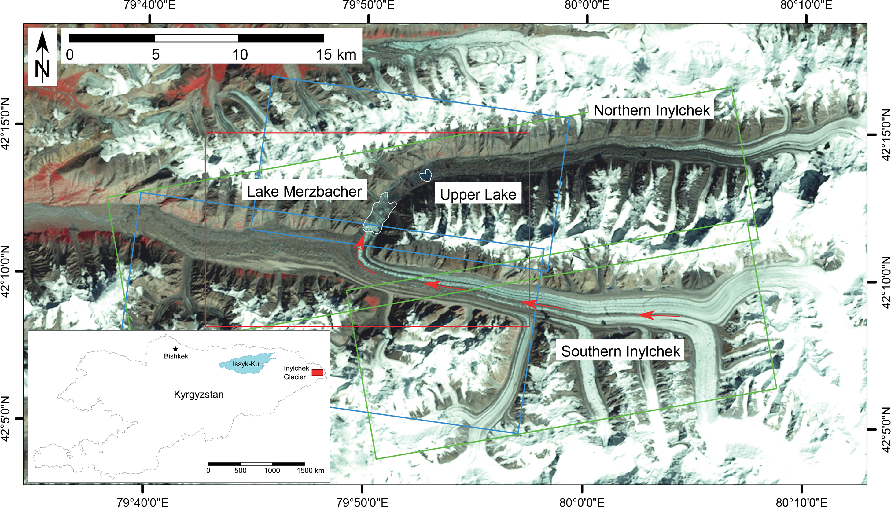
The Inylchek Glacier is located in the central Tien Shan mountain range between 42°4′N, 79°39′E and 42°15′N, 80°12′E. It consists of two heavily debris-covered glacial branches, called the Northern and Southern Inylchek, which flow out of the Podeba–Khan Tengri mountain massif towards the west (Figure 1). The entire system stretches over 60 km and covers an area of approximately 800 km2 [10], at altitudes between 2900 m and 7400 m [14]. Our study focuses on the ablation region of Southern Inylchek, which is rather flat with a mean slope of 2°.
Glacial lakes are located in the valley between the two branches. The larger of them, Lake Merzbacher, covers an area of approximately 5.6 km2 and is prevented from flowing downwards into the Inylchek valley by the Southern Inylchek, which acts as a dam across the lake. The lake drains annually with a glacial lake outburst flood (GLOF), thereby causing a sudden flooding of urban areas in Tarim basin further downstream [15–17].
Previous remote sensing studies based on Environmental Satellite Advanced Synthetic Aperture Radar (ENVISAT ASAR) data [18], ASTER imagery [10], and ASTER as well as Landsat TM scenes [19] indicate surface flow velocities of the upper Southern Inylchek of about 100 m/yr westwards, which corresponds to approximately 27 cm/d. At the confluence of the Northern and Southern Inylchek valleys (Figure 2), a part of the Southern Inylchek branch turns northwards and calves a substantial amount of ice into Lake Merzbacher. The remaining glacier mass continues to flow towards the west and is termed as lower part of Southern Inylchek within this study. This lower area and—even more pronounced—also Northern Inylcheck are rather stagnant and show only slow motions of several m/yr to the west.
In addition to the remote sensing observations, discrete points marked on the glacier surface have been repeatedly surveyed with differential GPS—the Global Positioning Satellite System—during the summer months [10], that generally confirm the annual mean flow characteristics obtained from the satellite data. Moreover, one remotely operated multi-parameter station has been installed directly on the glacier surface close to Lake Merzbacher’s ice dam in summer 2010. This station continuously provides Global Navigation Satellite System (GNSS) data, showing for example a late autumn month surface velocity of around 15 cm/d [20]. Further geodetic and hydrometeorological instruments are installed at the Global Change Observatory “Gottfried Merzbacher” that is located at the confluence of the Northern and Southern Inylchek valleys.
3. Data and Methodology
3.1. TerraSAR–X Data Set
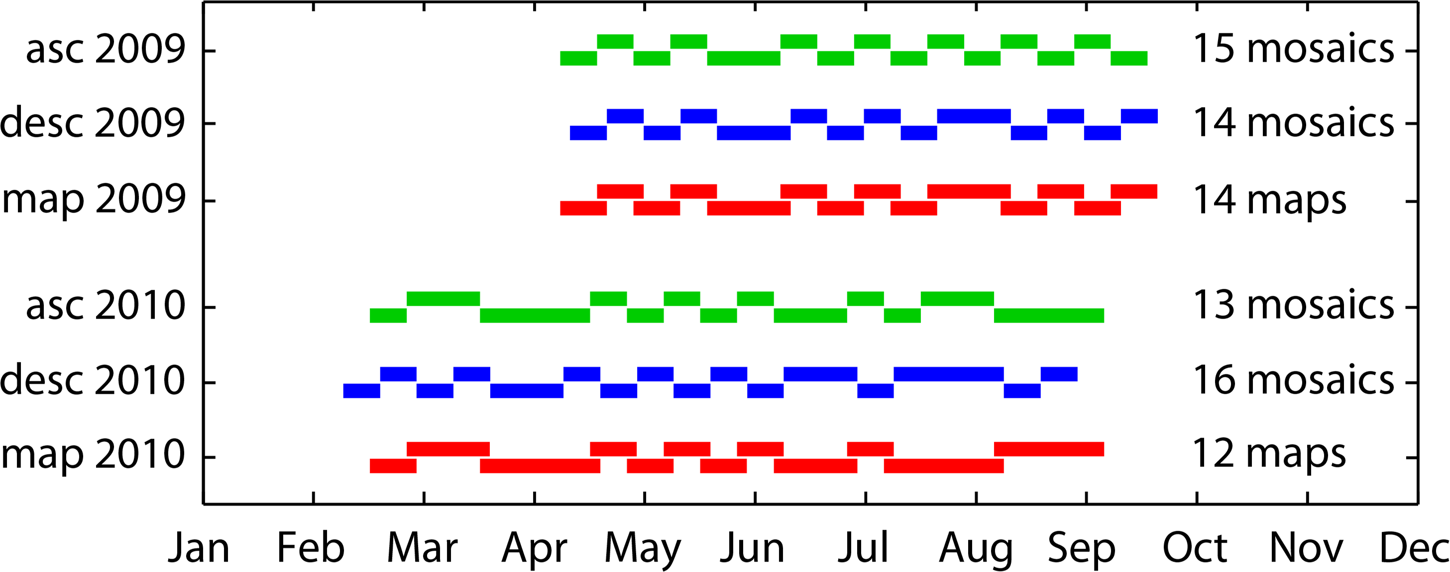
We process 116 image pairs from a total of 124 acquisitions gained in Stripmap mode and single polarisation (HH) from the TerraSAR–X satellite. The data has been taken from both ascending and descending orbits with incident angles of 22° and 35° and satellite heading angles of 350° and 188°, respectively, and covers the spring to autumn seasons of both 2009 and 2010 (Table 1). Pixel spacing is approximately 0.9 m in range and 2.0 m in azimuth direction, except for the descending acquisitions in 2010, where pixel spacing in range direction is only 1.4 m. At each acquisition date, two adjacent scenes have been taken that are mosaiced after performing the feature tracking procedure as outlined in the next section. The temporal baseline between two acquisitions is typically 11 days, with occasionally longer baselines of up to 33 days due to missing acquisitions. Displacements obtained from range and azimuth observations for both orbits are subsequently combined to finally arrive at 3D velocity estimates of the glacier surface (Figure 3).
3.2. Feature Tracking
The InSAR methodology has been commonly applied for investigating surface displacements from satellite radar data [21,22]. Typical application examples besides glacier kinematics [23–25] are earthquakes [26–28], landslides [29–31] or volcanic deformation [32–34]. However, InSAR works only over regions that are not affected by decorrelation due to surface changes between two acquisitions. Regarding our study area, we note that coherence between image pairs is rather poor for fast flowing glaciers as Inylchek, in particular during summer months where also surface melting extensively alters the phase component of the radar signal. We therefore apply the feature tracking method [13], which does not rely on the phase, but only takes the backscattered intensity information of the radar image into account. The method has already been previously applied to derive glacier surface motions [4,35,36]. To process the data, we used the algorithm implemented in the SARscape software package [37].
As a first step, coregistration is performed individually on each image pair, whereas the earlier acquisition always acts as the master image. To gain sub-pixel accuracy, which is a requirement for a precise image comparison [38], the registration is performed in a two-step procedure including coarse and fine coregistration, by which we achieve a final accuracy of 1/10 of a pixel. In the next step, horizontal shifts between intensity backscatters within the image pairs are computed based on identifying the maximum in normalised cross-correlation functions of small image patches, that are additionally oversampled by a factor of 16 for increased spatial resolution. The accuracy of the method is, however, highly dependent on distinguishable features within the intensity data [13].
For our application, we select window shifts of 10 and 12 pixels in range and azimuth, respectively, for all ascending and 2010 descending acquisitions. For descending acquisitions acquired in the year 2009, we use a shift of 15 pixels in range direction, thereby achieving a ground resolution of approximately 25 m in all our results. The size of the small image patch that contributes to the average cross-correlation function is chosen to be 32 pixels in both range and azimuth. To avoid noisy results in areas dominated by features rather indistinguishable in the intensity data, identified maxima with cross-correlations below 0.2 are discarded and set to no data in the offset images.
Offset values are subsequently converted into metric units by applying the associated pixel spacing values, and images are geocoded with the aid of a SRTM digital elevation model (DEM) [39]. The DEM’s original resolution of 90 m has been upsampled to an output resolution of 25 × 25 m which is in line with the selected window shifts applied during the feature tracking. The average amount of the SRTM geocoding error over Asia is specified as ±8.8 m [40] which is about one third of the output resolution and hence does not affect our results. Displacement maps are mosaiced for the two adjacent scenes acquired on the same date, whereas the overlapping region is re-calculated by averaging the corresponding displacements from the upper and lower scene. Finally, averaged daily velocities are calculated by dividing displacement rates by the length of the temporal baseline for each mosaic.
Failure of the cross-correlation leads to erroneous results that contain extreme values. To prevent further processing with the corresponding pixels in the tracking results, those are set to missing values according to a threshold which is calculated from the mean (μ) of all values and the standard deviation (σ) for each individual mosaic. Every value that does not fall within the range μ ± 3σ is rejected. We are aware that the tracking values are not entirely normally distributed due to a systematic difference between stable bedrock and moving glacial areas. However, the 3σ criterion is large enough to preserve all realistic displacements. Still, there remain regions that are affected by shadowing or layover in either the ascending and descending acquisitions. Based on the value of the local incidence angle of the radar beam, a mask has been created, whereas values with negative sign are assumed to be layover areas and values greater than 90° represent shadow areas. Accordingly, regions with local incidence angles that fall either in the layover or shadow range are rejected to prevent interpretation of erroneous displacement estimates.
3.3. Decomposition to 3D Velocities
Since in principle four one-dimensional estimates of displacements are available from range and azimuth images of ascending and descending acquisitions for a given time interval, it is straightforward to combine them into a single estimate of 3D velocities. For a right-looking system like TerraSAR-X the displacements in azimuth dazi are noted as:
The decomposition formula is applied to the offset mosaics that had in advance been trimmed to the same spatial extend. As a result, we gain the 3D information containing vertical and horizontal motion components of the surface glacier flow. In a final processing step, we smooth the images by applying a 5 × 5 boxcar filter.
Since 3D velocities are obtained from combining image pairs from both ascending and descending orbits that are acquired with a minimum delay of 3 days, we note that the 3D velocity estimates presented below must be interpreted as average displacement rates representative for a time-period of 14 days under ideal circumstances. If the temporal baseline of an image pair is longer due to missing acquisitions, the averaging period increases accordingly. Within this study, no differentiating between horizontal and vertical motion components has been undertaken, instead results focus on the absolute value (i.e., the speed) of the derived 3D velocity vector.
4. Results
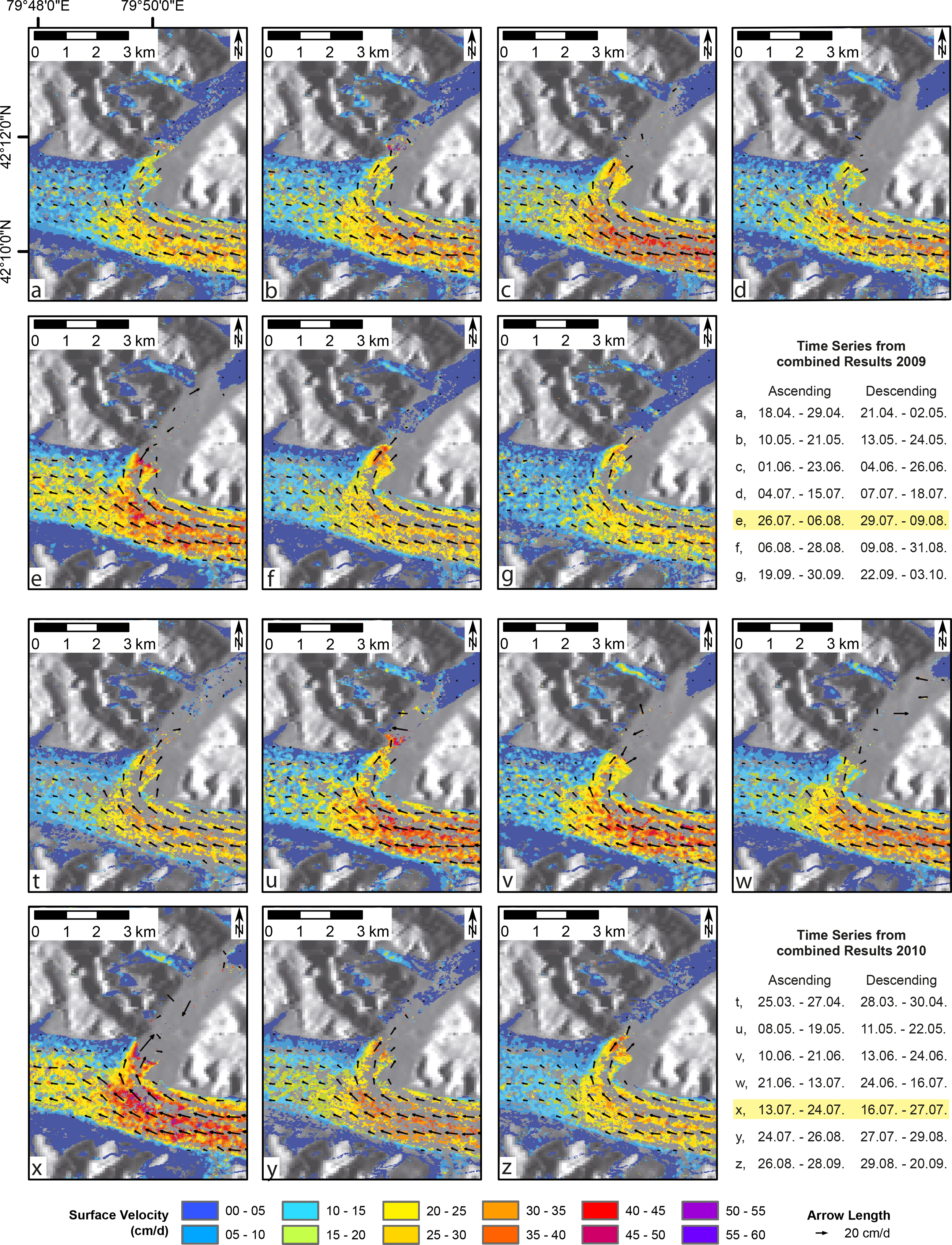
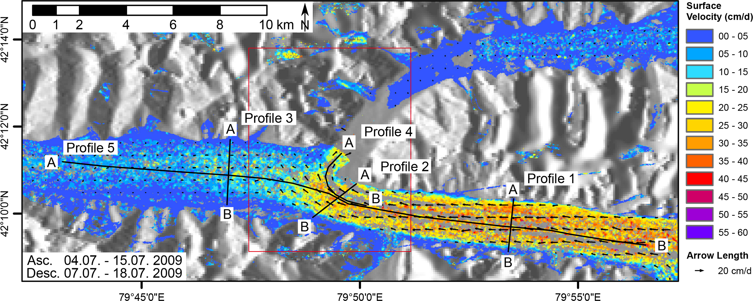
A snap-shot from July 2009 is representative for the flow regime of Inylchek glacier during the summer months (Figure 4). Velocities between 25 to 50 cm/d towards the west are apparent in the upper part of Southern Inylchek, whereas the lower part and Northern Inylchek show substantially smaller surface movements. The bending of the surface flow towards north in the direction of Lake Merzbacher at the confluence of the valleys is clearly visible. Besides those general features, surface velocities vary significantly both across the glacier and also in direction of the mean flow, potentially providing additional high-resolution information of the flow field.
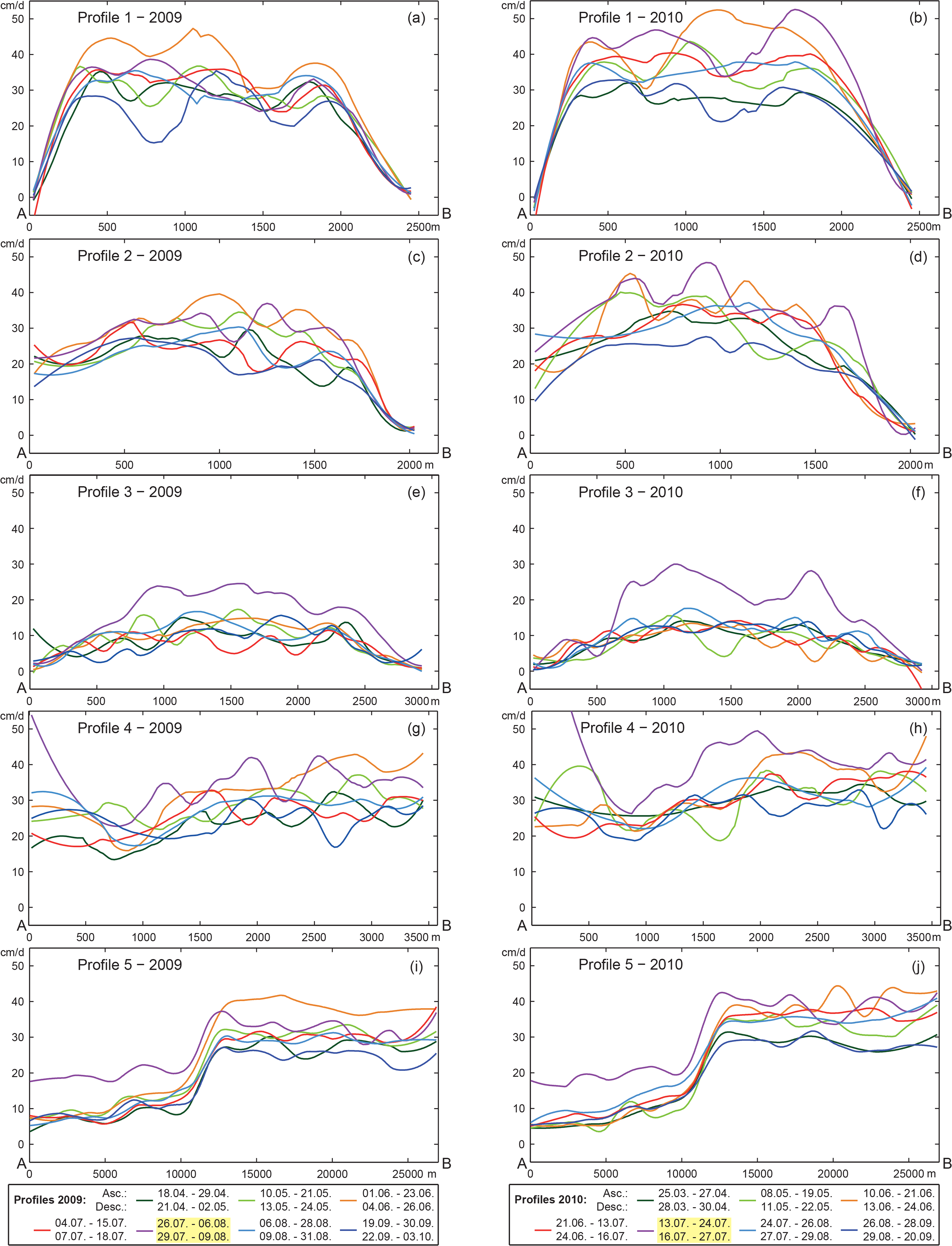
From our time-series of displacement fields and hence surface motions, we present a number of snap-shots for the bending region at the valley confluence, which is presumably the glaciologically most interesting area of the glacier system (Figure 5). Two time-periods with peak velocities are recognisable: one appears in June, as we observe motion rates in the upper part of the glacier at approximately 40 cm/d for both years (Figure 5c,v). The second peak occurs during the summer season with velocity rates of 40 cm/d in July/August 2009 (Figure 5e) and 50 cm/d in July 2010 (Figure 5x). After the occurrence of this major peak in the summer, the glacier slows down substantially, with mean displacement rates of 25 cm/d in September 2009 (Figure 5g) and 2010 (Figure 5z).
To allow for a more quantitative comparison, we present five profiles, that are well distributed over the Southern Inylchek branch (Figure 6). Their locations are marked in Figure 4. Three of the profiles are perpendicular to the main flow direction: profile 1 represents a cross-section of the upper area, profile 2 shows a cross-section in the bending region and profile 3 gives information about the velocity variations in the lower part of the glacier. Two additional profiles oriented parallel to the glacier show the changes of the kinematic behaviour along the flow direction. Profile 4 illustrates the ice flow turning towards the north in the bending area, and profile 5 gives an overview of nearly the entire investigation area of the Southern Inylchek branch, particularly demonstrating the motion variance between the upper and lower parts of the glacier.
In the upper area of Southern Inylchek glacier, the general alignment of the velocity rates perpendicular to the glacier flow shows roughly a typical maximum value close to the center axis of the glacier, with strongly decreased values towards the margins. However, in the broad middle area, many variations are distinguishable, reaching from a minimum of 20 cm/d up to a maximum of 50 cm/d during the seasons (profile 1 in Figure 6a,b). The same profile reveals that besides these variances a rising trend of the surface velocity from spring to summer is observable: spring mean values are at 25 cm/d, whereas the summer mean is found at 35–40 cm/d. Distinct peaks appear in June within both 2009 and 2010 with a maximum of 50 cm/d. Autumn values are again substantially reduced to 25–30 cm/d in both years. Particularly evident are differences at the southern margin of the glacier. In 2009, the maximum in this area is approximately 35 cm/d. In 2010, the surface of the glacier has moved much faster, yielding values of up to 50 cm/d.
At the beginning of the bending area, the incoherent motion pattern of the parallel glacial streams is still apparent, albeit with 20 % lower values (profile 2 in Figure 6c,d). Below the confluence area, the glacier body moves in a more uniform way, as cross-alignment variations are unincisive. The glacier velocity has slowed down and surface displacements do not vary too much during the year: the velocity rates for both 2009 and 2010 are approximately 5–10 cm/d (cp. profile 3 in Figure 6e,f). Nevertheless, the second peak observed in the upper area in the snap-shot images is also apparent in this region, resulting in significantly increased velocity rates of 20–25 cm/d.
The behaviour in the transitional area between the upper and the lower part of the glacier is shown in profile 4 (Figure 6g,h). However, some limitations have to be considered when analysing this part: the bending area is highly affected by layover effects of the nearby mountains. Thus this part of the area is masked out and cannot be interpreted. Still, the profile reveals a distinct decrease of the glacier surface flow velocity, from values of approximately 30–40 cm/d to approximately 20–30 cm/d in the middle of the bending area. On the contrary, an increasing velocity trend is observable after the ice has changed its flow direction, resulting in a faster movement of the glacier towards the lake. The strong velocity increase in summer already seen in profile 3 is also apparent directly at the calving front, where the glacier moves with a sudden rush towards Lake Merzbacher during the time of the second peak (Figure 5e,x, Figure 6g,h).
Profile 5 (Figure 6i,j) finally shows the overall situation, where once again the significant surface velocity drop is apparent below the bending area. It is evident that seasonal changes appear within the upper part of Southern Inylchek glacier, but barely within the lower area except for the time of the second peak. This major event occurring in August 2009 and July 2010 affects the entire region below the confluence area, whereas maximum values in the upper region appear rather earlier during June, which is especially distinctive in 2009.
5. Discussion
5.1. Error Estimation
Before discussing the variations of the surface velocity in detail, an attempt is made to estimate the magnitude of the error in our results. Based on the assumption that a non-glacier area not affected by motion should yield velocity values spanning around zero [4,38], we analysed the kinematic results of the small surface patch between the two lakes. For 2009, the average mean velocity for that region over all scenes is 2.04 cm/d with an average standard deviation of 1.19 cm/d. For 2010, the values are similar, with an average mean of 2.17 cm/d and a corresponding average standard deviation of 1.15 cm/d. Both years independently show comparable mean offset errors that are ten times lower than the calculated glacier velocity, which indicates that all signals larger than a few cm/d are well above the noise level.
Geocoding of the tracking results has been achieved with the help of the SRTM-DEM that had been acquired in 2000. Assuming that similar to the neighbouring Tomur Glacier [43], the Inylchek height was also lowered by approximately 15 m between 1999 and 2009 and neglecting earth curvature, the geocoding error ∊ that is introduced by a DEM height difference δH can be calculated as follows:
Thus, for the incident angles of θa =22° and θd =35° the geocoding error would be 37 m and 21 m, respectively. This roughly corresponds to the final resolution of our images and therefore alters the results only marginally, since it just affects the position of a line-of-sight displacement, but not the displacement vector itself.
5.2. Inter-Annual Kinematics of the Upper Southern Inylchek Glacier Branch
Kinematic variations found perpendicular to the glacier main flow in the upper part of the Southern Inylchek branch indicate independent moving behaviour of adjacent longitudinal streams. The strong velocity increase at the southern margin of the glacier from 2009 to 2010 has been already described in [19] and seems to be related to a decrease in the glacial flow of the adjacent glacier tributary.
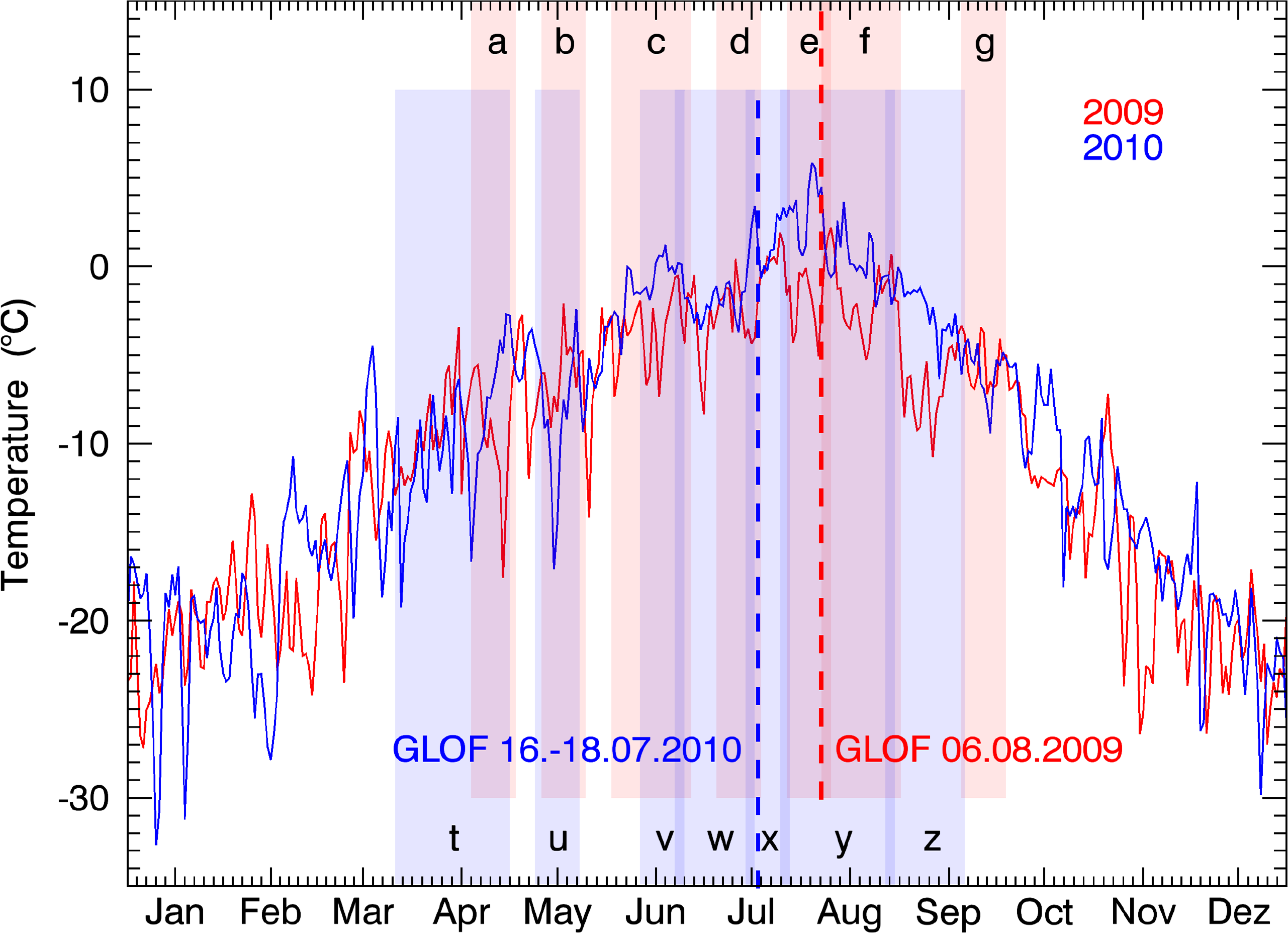
To explain the general surface motion increase from April to June over the upper Southern Inylchek branch, we include air temperature data from the European Centre for Medium-Range Weather Forecasts (ECMWF) global operational analysis (Figure 7). Within the data from the numerical weather prediction model, we observe in both 2009 and 2010 a constant increase of air temperatures beginning in March, reaching peak values in July/August. Together with a simultaneously occurring increase in precipitation (not shown), the air temperature increase intensifies the ablation process on the glacier’s surface [44]. Through the accelerated melting of the snow situated on the surrounding mountains and on the glacier itself, additional water is introduced to the system, which penetrates into the ice by means of crevasses and fractures and drains through subglacial ice tunnels. If the amount of melt water is comparatively high, these passageways are not able to adjust their size quick enough to the water flux. As a consequence, the pressure and the volume of the water at the basal base increases, leading to a reduction of the frictional strength and ultimately to an increase of the basal sliding of the glacier [45–47].
The comparison between averaged daily surface velocities and daily air temperature values provides an explanation for the slightly higher kinematics in 2010 than in 2009 (cp. Profile 5 in Figure 6i,k). At the beginning of the spring season in March/April (cp. Figure 5a,t) velocity values are still approximately the same in both years, although the corresponding time frame is different. In 2010 the spring result covers a time period of 36 days while in 2009 it covers a time period of 14 days, which temporally fall into the later part of the 2010 result. We thus would expect higher surface velocities in 2009 than in 2010. However, by looking at Figure 7, we realise that the corresponding mean air temperatures in both years are approximately the same, which may explain the similar velocities that we observe in spring 2009 and 2010.
In the middle of May, we see distinctive velocity differences in the bending area of the glacier between 2009 and 2010 (Figure 5b,u); in 2009 the glacier surface moves with 30–35 cm/d while in 2010 kinematics speed up to 40 cm/d. However, air temperature values for the same time span appear rather vice versa: the mean temperature value for 2009 is −6 °C while for 2010 we observe a sharp drop in the temperature from −4 °C to −17 °C followed by a quick rise to −3 °C within two weeks. Therefore, we would expect rather lower surface velocity values in 2010. However, as seen in Figure 7, we observe an apparent peak in the air temperature just the week before the corresponding 2010 acquisitions, which lasts for several days and is clearly higher than temperature values for the same time period in 2009. We thus assume that the higher glacier kinematics in May 2010 should be interpreted as an aftermath of this rather warm period.
Figure 5c,v as well as the Profile 5 in Figure 6i,j show for both years surface motion values around 40 cm/d in June. Air temperatures for the corresponding time period do not substantiate this development, since mean values in 2010 are −1 °C, which is clearly higher than the mean of −4 °C in 2009. A possible explanation might be the noticeable difference in the amount of precipitation values that could have a favourable effect on the glacier motion: in 2009 we have accumulated monthly values of 116 mm as compared to only 73 mm in 2010 (not shown here).
From June on, air temperatures are constantly higher in 2010 than in 2009, reaching values even above the freezing point in July and August (maximum: 6 °C), whereas values in 2009 are most of the time just below 0 °C. Air temperatures above the freezing point have a profound effect on surface melting [48], in turn allowing a significant amount of melt water to be introduced into the system in summer 2010. Accordingly, mean summer 2010 velocities are mainly higher than those in 2009: 30 cm/d for July 2009 vs. 37 cm/d for July 2010 and 35 cm/d for August 2009 vs. 40 cm/d for August 2010 (Figure 6i,j). A convergence of the kinematics towards a mean of 25 cm/d is only observable in September again.
In summary, evidence presented above leads to the conclusion that for the upper part of the Southern Inylchek Glacier branch the amount of surface velocity correlates most of the time with air temperature. Especially air temperatures above the freezing point seem to induce an increased glacier flow. A comparable general correlation over the time with precipitation has not been found so far.
5.3. Lake Level Extent and GLOF
Because calm water reflects the radar beam away from the sensor, cross-correlation values over the area of Lake Merzbacher fall below the defined 0.2 threshold. As a consequence, most of the lake area is masked out during the processing. Single features that are still visible are likely to be related to ice bergs floating on the surface. By looking at the boundary of this no-data area in combination with the DEM, it is possible to extract information about the water level of the lake.
After applying the layover/shadow mask, no-data values due to the mask are overlapping those that are related to the missing backscatter information due to the outline of the lake. However, the maximum extent of Lake Merzbacher towards the Northern Inylchek branch is clearly visible. The results from the spring period show just a small no-data area in the study area (Figure 5b,u), which indicates that only a marginal amount of liquid water is present. With time, the outline of this gap increases, reaching its maximum extent in the summer, which correlates with the time of the appearance of the second velocity peak (Figure 5e,x). Along with the strong decline of the glacier surface velocity directly after this peak, backscatter intensities are observed again for the lake area, leading to the conclusion that the water must have drained away (Figure 5f,y). After this point, no apparent changes in the low water level are recognisable during the autumn season.
From in-situ observations collected at the Global Change Observatory “Gottfried Merzbacher”, it is known that GLOF events of Lake Merzbacher took place on both 6 August 2009, and between 16–18 July 2010. Both events coincide well with the increased velocities of the lower part of Southern Inylchek (Figure 6i,j). We assume that at the beginning of the GLOF, the existing drainage tunnels of the Inylchek glacier are not large enough to allow an immediate discharge of the lake water. Thus, the significant increase of the subglacial water pressure lubricates the bed allowing for a basal sliding over large areas [45]. Similar to [49], who monitored a GLOF-induced glacier velocity increase in Iceland, we observe a strong speed-up in the bending area and particularly in the lower area, since these are the regions directly affected by the draining water. Therefore, it can be implied that the GLOF directly influences the glacier’s kinematics by triggering a so-called mini-surge. A mini-surge is characterised by at least a double speed velocity and lasts for a time period of approximately one day [50]. As illustrated in Section 4, the velocity has increased by more than 100% in the lower part of the glacier, from approximately 5–10 cm/d before the GLOF to 25 cm/d during the GLOF. However, it should be noted that these values are only averaged results over an 14-day time period. Thus, we expect an even higher displacement rate during the actual draining period, since the main flooding event occurs only within a couple of days.
By comparing the dates of the GLOF events between 2009 and 2010, we note an earlier draining of the lake for about three weeks in 2010. This is easily explained by the air temperatures above the freezing point in summer 2010. The high temperatures lead to increased snow melting as well as surface melting of the glacier itself. Following on, a large amount of water is introduced to the system, which lets the water level of Lake Merzbacher rise more quickly. As a consequence, the water pressure reaches its critical threshold earlier as in 2009, which finally results in the earlier flooding.
6. Conclusions
In this study, radar data have been used to observe seasonal surface velocity variations of the Inylchek Glacier in Kyrgyzstan. We demonstrated that detailed monitoring of spatial and temporal kinematics variability with TerraSAR–X is feasible due to the satellites’ relatively short repetitive cycle of 11 days and the independence from solar illumination or atmosphere conditions. Another major advantage of using TerraSAR–X data is the high spatial resolution. By using Stripmap images with an original resolution of 3 m, we are able to generate final products with a resolution of 25 m that show not only the general mean velocity of the main glacier but also allows us to detect kinematic differences between individual longitudinal streams. We applied the feature tracking method to calculate the velocity field of the glacier, which yields sufficient information to derive a complete overview of the displacement of the entire glacier surface. By taking into account data from ascending and descending orbits, it is possible to derive 3D information about the kinematics.
For the observed period of 2009 and 2010, the seasonal displacement investigation for the ablation area of Southern Inylchek Glacier shows velocity rates from 25 to 50 cm/d for the active upper part, with small changes in perpendicular flow direction. In general, lowest surface velocity values are found during April and September, whereas in May an increase of the motion rates is observed. A first velocity peak appears for both years in June with a mean of 40 cm/d. Comparison to daily air temperatures reveals a general correlation between temperature and glacier surface flow. In 2010, we observe that summer air temperatures above the freezing point lead to a significant velocity increase: mean values in 2010 are 15% higher than in 2009. In addition, the onset of the annually occurring glacial lake outburst flood (GLOF) of Lake Merzbacher is three weeks earlier in 2010 as compared to 2009.
The motion of the lower region of the Southern Inylchek branch appears homogeneously, with constant velocity rates of 5–10 cm/d over the year. This displacement rate only changes when the branch is affected by the GLOF that is associated with the second velocity peak. During the outburst, the surface kinematics increase with values reaching 25 cm/d, which is more than twice the normal rate and thus is termed as a mini-surge.
As a consequence, we conclude that the drainage of Lake Merzbacher, inducing the water to flow underneath the ice body, has a large impact on the Southern Inylchek’s movement behaviour. The source of the mini-surge is likely to be related to the rise of the water pressure at the glacier’s bottom, reducing the friction between ice and solid ground, leading to an increase of the basal slip and therefore the glacier’s velocity.
Our study gave evidence that in the future, large-scale monitoring of changes in seasonal surface kinematics of glaciers will help to improve the understanding of a glacier’s behaviour. The small and short-time, yet distinctive, velocity change characteristics could be used for example as additional input to improve or validate mass-balance estimation models by for instance applying the vertical velocity component like proposed in [51]. They could also serve as a constraint for estimating ice thickness and glacier bed topography [52] or for modelling the spatial distribution of the surface-to-bed meltwater transfer [53]. Furthermore, information about the speed of glacial lake filling could be used to refine GLOF prediction models, like the one developed by [54] for the Merzbacher Lake.
For the Inylchek area, the relation between glacier alignment, tributary ice input, GLOF event, and hydrometeorological variations, and how each influences the development of the glacier’s motion is not yet fully understood. Close monitoring with high spatial and temporal resolution of the surface kinematics in connection with further hydrometeorological in-situ observations will be a basis to gain further insight into Inylchek’s glacial processes.
Acknowledgments
The authors would like to thank the anonymous reviewers for their helpful comments and suggestions to improve the quality of this paper. This study is supported by the German Federal Ministry of Research and Technology (BMBF) via the project PROGRESS (Potsdam Research Cluster for Georisk Analysis, Environmental Change and Sustainability) and by the Initiative and Networking Fund of the Helmholtz Association in the frame of Helmholtz Alliance “Remote Sensing and Earth System Dynamics”. The TerraSAR–X data are kindly provided by the German Aerospace Center (DLR) under the proposal number HYD0289. The Landsat TM scene is made available from the U.S. Geological Survey.
Author Contributions
Julia Neelmeijer designed the research, processed the remote sensing data and wrote the main part of the manuscript. Mahdi Motagh was responsible for the scientific supervision on the development process and contributed to the manuscript writing. Hans-Ulrich Wetzel contributed to the data analyses and the manuscript writing.
Conflicts of Interest
The authors declare no conflict of interest.
References
- Aizen, V.B.; Aizen, E.M.; Kuzmichonok, V.A. Glaciers and hydrological changes in the Tien Shan: Simulation and prediction. Environ. Res. Lett 2007, 2. [Google Scholar] [CrossRef]
- Aizen, V.B.; Kuzmichenok, V.A.; Surazakov, A.B.; Aizen, E.M. Glacier changes in the Tien Shan as determined from topographic and remotely sensed data. Glob. Planet. Chang 2007, 56, 328–340. [Google Scholar]
- Bolch, T. Climate change and glacier retreat in northern Tien Shan (Kazakhstan/Kyrgyzstan) using remote sensing data. Glob. Planet. Chang 2007, 56, 1–12. [Google Scholar]
- Li, J.; Li, Z.; Zhu, J.; Ding, X.; Wang, C.; Chen, J. Deriving surface motion of mountain glaciers in the Tuomuer-Khan Tengri Mountain Ranges from PALSAR images. Glob. Planet. Chang 2013, 101, 61–71. [Google Scholar]
- Narama, C.; Kääb, A.; Duishonakunov, M.; Abdrakhmatov, K. Spatial variability of recent glacier area changes in the Tien Shan Mountains, Central Asia, using Corona (∼ 1970), Landsat (∼ 2000), and ALOS (∼ 2007) satellite data. Glob. Planet. Chang 2010, 71, 42–54. [Google Scholar]
- Kutuzov, S.; Shahgedanova, M. Glacier retreat and climatic variability in the eastern Terskey-Alatoo, inner Tien Shan between the middle of the 19th century and beginning of the 21st century. Glob. Planet. Chang 2009, 69, 59–70. [Google Scholar]
- Erten, E.; Reigber, A.; Hellwich, O.; Prats, P. Glacier Velocity Monitoring by Maximum Likelihood Texture Tracking. IEEE Trans. Geosci. Remote Sens 2009, 47, 394–405. [Google Scholar]
- Fallourd, R.; Harant, O.; Trouvé, E.; Nicolas, J.-M.; Gay, M.; Walpersdorf, A.; Mugnier, J.-L.; Serafini, J.; Rosu, D.; Bombrun, L.; et al. Monitoring Temperate Glacier Displacement by Multi-Temporal TerraSAR-X Images and Continuous GPS Measurements. IEEE J. Sel. Top. Appl. Earth Obs. Remote Sens 2011, 4, 372–386. [Google Scholar]
- Aizen, V.B.; Aizen, E.M.; Dozier, J.; Melack, J.M.; Sexton, D.D.; Nesterov, V.N. Glacial regime of the highest Tien Shan mountain, Pobeda-Khan Tengry massif. J. Glaciol 1997, 14, 503–512. [Google Scholar]
- Mayer, C.; Lambrecht, A.; Hagg, W.; Helm, A.; Scharrer, K. Post-drainage ice dam response at Lake Merzbacher, Inylchek glacier, Kyrgyzstan. Geogr. Ann. Series A Phys. Geogr 2008, 90, 87–96. [Google Scholar]
- Andersen, M.L.; Larsen, T.B.; Nettles, M.; Elosegui, P.; van As, D.; Hamilton, G.S.; Stearns, L.A.; Davis, J.L.; Ahlstrøm, A.P.; de Juan, J.; et al. Spatial and temporal melt variability at Helheim Glacier, East Greenland, and its effect on ice dynamics. J. Geophys. Res 2010, 115, F04041. [Google Scholar]
- Haemmig, C.; Huss, M.; Keusen, H.; Hess, J.; Wegmüller, U.; Ao, Z.; Kulubayi, W. Hazard assessment of glacial lake outburst floods from Kyagar glacier, Karakoram mountains, China. Ann. Glaciol 2014, 55, 34–44. [Google Scholar]
- Strozzi, T.; Luckman, A.; Murray, T.; Wegmüller, U.; Werner, C.L. Glacier motion estimation using SAR offset-tracking procedures. IEEE Trans. Geosci. Remote Sens 2002, 40, 2384–2391. [Google Scholar]
- Hagg, W.; Mayer, C.; Lambrecht, A.; Helm, A. Sub-debris melt rates on southern Inylchek Glacier, central Tian Shan. Geogr. Ann. Series A Phys. Geogr 2008, 90, 55–63. [Google Scholar]
- Wang, R.; Gao, Q. Preliminary study on flash floods in Tarim River basin. Chin. Geogr. Sci 1997, 7, 53–58. [Google Scholar]
- Jingshi, L.; Fukushima, Y. Recent change and prediction of glacier dammed lake outburst floods from Kunmalik River in southern Tien Shan, China. In Hydrological Extremes: Understanding, Predicting, Mitigating; Gottschalk, L., Olivry, J.-C., Reed, D., Rosbjerg, D., Eds.; IAHS Publisher: Birmingham, UK, 1999; pp. 99–107. [Google Scholar]
- Glazirin, G.E. A century of investigations on outbursts of the ice-dammed Lake Merzbacher (central Tien Shan). Austrian J. Earth Sci 2010, 103, 171–179. [Google Scholar]
- Wetzel, H.-U.; Reigber, A.; Richter, A.; Michajljow, W. Gletschermonitoring und Gletscherseebrüche am Inyltschik (Zentraler Tienshan)—Interpretation mit optischen und Radarsatelliten. In GEO-GOVERNMENT - Wirtschaftliche Innovation durch Geodaten: Vorträge; 25. Wissenschaftlich-Technische Jahrestagung der DGPF; Seyfert, E., Ed.; Publikationen der Deutschen Gesellschaft für Photogrammetrie, Fernerkundung und Geoinformation e.V.: Potsdam, Germany, 2005; pp. 341–350. [Google Scholar]
- Nobakht, M.; Motagh, M.; Wetzel, H.-U.; Roessner, S.; Kaufmann, H. The Inylchek Glacier in Kyrgyzstan, Central Asia: Insight on surface kinematics from optical remote sensing imagery. Remote Sens 2014, 6, 841–856. [Google Scholar]
- Zech, C.; Schöne, T.; Neelmeijer, J.; Zubovich, A.; Galas, R. Geodetic monitoring networks: GNSS-derived glacier surface velocities at the Global Change Observatory Inylchek (Kyrgyzstan). In Proceedings of the 2013 IAG General Assembly, Potsdam, Germany, 1–6 September 2013.
- Bamler, R.; Hartl, P. Synthetic aperture radar interferometry. Inverse Probl 1998, 14, 1–54. [Google Scholar]
- Rosen, P.A.; Hensley, S.; Joughin, I.R.; Li, F.K.; Madsen, S.N.; Rodriguez, E.; Goldstein, R.M. Synthetic aperture radar interferometry. Proc. IEEE 2000, 88, 333–382. [Google Scholar]
- Mohr, J.J.; Reeh, N.; Madsen, S.N. Three-dimensional glacial flow and surface elevation measured with radar interferometry. Nature 1998, 391, 273–276. [Google Scholar]
- Joughin, I.; Smith, B.E.; Abdalati, W. Glaciological advances made with interferometric synthetic aperture radar. J. Glaciol 2010, 56, 1026–1042. [Google Scholar]
- Mouginot, J.; Scheuchl, B.; Rignot, E. Mapping of ice motion in Antarctica using Synthetic-Aperture Radar data. Remote Sens 2012, 4, 2753–2767. [Google Scholar]
- Fialko, Y.; Simons, M.; Agnew, D. The complete (3-D) surface displacement field in the epicentral area of the 1999 MW 7.1 Hector Mine Earthquake, California, from space geodetic observations. Geophys. Res. Lett 2001, 28, 3063–3066. [Google Scholar]
- Satyabala, S.P.; Yang, Z.; Bilham, R. Stick-slip advance of the Kohat Plateau in Pakistan. Nat. Geosci 2012, 5, 147–150. [Google Scholar]
- Motagh, M.; Beavan, J.; Fielding, E.J.; Haghshenas, M. Postseismic ground deformation following the September 2010, Darfield, New Zealand, earthquake from TerraSAR-X, COSMO-SkyMed, and ALOS InSAR. IEEE Geosci. Remote Sens. Lett 2014, 11, 186–190. [Google Scholar]
- Strozzi, T.; Farina, P.; Corsini, A.; Ambrosi, C.; Thüring, M.; Zilger, J.; Wiesmann, A.; Wegmüller, U.; Werner, C. Survey and monitoring of landslide displacements by means of L-band satellite SAR interferometry. Landslides 2005, 2, 193–201. [Google Scholar]
- Akbarimehr, M.; Motagh, M.; Haghshenas-Haghighi, M. Slope stability assessment of the Sarcheshmeh Landslide, Northeast Iran, investigated using InSAR and GPS observations. Remote Sens 2013, 5, 3681–3700. [Google Scholar]
- Motagh, M.; Wetzel, H.-U.; Roessner, S.; Kaufmann, H. A TerraSAR-X InSAR study of landslides in southern Kyrgyzstan, Central Asia. Remote Sens. Lett 2013, 4, 657–666. [Google Scholar]
- Lu, Z.; Wicks, C.; Dzurisin, D.; Thatcher, W.; Freymueller, J.T.; McNutt, S.R.; Mann, D. Aseismic inflation of Westdahl Volcano, Alaska, revealed by satellite radar interferometry. Geophys. Res. Lett 2000, 27, 1567–1570. [Google Scholar]
- Lundgren, P.; Berardino, P.; Coltelli, M.; Fornaro, G.; Lanari, R.; Puglisi, G.; Sansosti, E.; Tesauro, M. Coupled magma chamber inflation and sector collapse slip observed with synthetic aperture radar interferometry on Mt. Etna volcano. J. Geophys. Res 2003, 108. [Google Scholar] [CrossRef]
- Anderssohn, J.; Motagh, M.; Walter, T.R.; Rosenau, M.; Kaufmann, H.; Oncken, O. Surface deformation time series and source modeling for a volcanic complex system based on satellite wide swath and image mode interferometry: The Lazufre system, central Andes. Remote Sens. Environ 2009, 113, 2062–2075. [Google Scholar]
- Quincey, D.J.; Copland, L.; Mayer, C.; Bishop, M.; Luckman, A.; Belò, M. Ice velocity and climate variations for Baltoro Glacier, Pakistan. J. Glaciol 2009, 55, 1061–1071. [Google Scholar]
- Paul, F.; Bolch, T.; Kääb, A.; Nagler, T.; Nuth, C.; Scharrer, K.; Shepherd, A.; Strozzi, T.; Ticconi, F.; Bhambri, R.; et al. The glaciers climate change initiative: Methods for creating glacier area, elevation change and velocity products. Remote Sens. Environ 2013. [Google Scholar] [CrossRef]
- Sarmap. Available online: http://www.sarmap.ch (accessed on 17 February 2014).
- Luckman, A.; Quincey, D.; Bevan, S. The potential of satellite radar interferometry and feature tracking for monitoring flow rates of Himalayan glaciers. Remote Sens. Environ 2007, 111, 172–181. [Google Scholar]
- Jarvis, A.; Reuter, H.I.; Nelson, A.; Guevara, E. Hole-Filled Seamless SRTM Data V4, 2008. Available online: http://srtm.csi.cgiar.org (accessed on 23 May 2014).
- Farr, T.G.; Rosen, P.A.; Caro, E.; Crippen, R.; Duren, R.; Hensley, S.; Kobrick, M.; Paller, M.; Rodriguez, E.; Roth, L.; et al. The shuttle radar topography mission. Rev. Geophys 2007, 45. [Google Scholar] [CrossRef]
- Nagler, T.; Rott, H.; Hetzenecker, M.; Scharrer, K.; Magnússon, E.; Floricioiu, D.; Notarnicola, C. Retrieval of 3D-glacier movement by high resolution X-band SAR data. In Proceedings of the 2012 IEEE International Geoscience and Remote Sensing Symposium (IGARSS), Munich, Germany, 22–27 July 2012; pp. 3233–3236.
- Muto, M.; Furuya, M. Surface velocities and ice-front positions of eight major glaciers in the Southern Patagonian Ice Field, South America, from 2002 to 2011. Remote Sens. Environ 2013, 139, 50–59. [Google Scholar]
- Pieczonka, T.; Bolch, T.; Wei, J.; Liu, S. Heterogeneous mass loss of glaciers in the Aksu-Tarim Catchment (Central Tien Shan) revealed by 1976 KH-9 Hexagon and 2009 SPOT-5 stereo imagery. Remote Sens. Environ 2013, 130, 233–244. [Google Scholar]
- Aizen, V.B.; Aizen, E.M.; Melack, J.M. Climate, snow cover, glaciers, and runoff in the Tien Shan, Central Asia. J. Am. Water Resour. Assoc 1995, 31, 1113–1129. [Google Scholar]
- Björnsson, H. Hydrological characteristics of the drainage system beneath a surging glacier. Nature 1998, 395, 771–774. [Google Scholar]
- Clarke, G.K.C. Subglacial processes. Annu. Rev. Earth Planet. Sci 2005, 33, 247–276. [Google Scholar]
- Cuffey, K.M.; Paterson, W.S.B. The Physics of Glaciers, 4th ed; Butterworth-Heinemann /Elsevier: Burlington, MA, USA, 2010. [Google Scholar]
- Sugiyama, S.; Skvarca, P.; Naito, N.; Enomoto, H.; Tsutaki, S.; Tone, K.; Marinsek, S.; Aniya, M. Ice speed of a calving glacier modulated by small fluctuations in basal water pressure. Nat. Geosci 2011, 4, 597–600. [Google Scholar]
- Magnússon, E.; Rott, H.; Björnsson, H.; Pálsson, F. The impact of jökulhlaups on basal sliding observed by SAR interferometry on Vatnajökull, Iceland. J. Glaciol 2007, 53, 232–240. [Google Scholar]
- Humphrey, N.; Raymond, C.; Harrison, W. Discharges of turbid water during mini-surges of Variegated Glacier, Alaska, USA. J. Glaciol 1986, 32, 195–207. [Google Scholar]
- Strozzi, T.; Gudmundsson, G.H.; Wegmüller, U. Estimation of the surface displacement of Swiss alpine glaciers using satellite radar interferometry. EARSeL eProc 2003, 2, 3–7. [Google Scholar]
- Mcnabb, R.W.; Hock, R.; O’Neel, S.; Rasmussen, L.A.; Ahn, Y.; Braun, M.; Conway, H.; Herreid, S.; Joughin, I.; Pfeffer, W.T.; et al. Using surface velocities to calculate ice thickness and bed topography: A case study at Columbia Glacier, Alaska, USA. J. Glaciol 2012, 58, 1151–1164. [Google Scholar]
- Clason, C.; Mair, D.W.F.; Burgess, D.O.; Nienow, P.W. Modelling the delivery of supraglacial meltwater to the ice/bed interface: application to southwest Devon Ice Cap, Nunavut, Canada. J. Glaciol 2012, 58, 361–374. [Google Scholar]
- Ng, F.; Liu, S. Temporal dynamics of a jökulhlaup system. J. Glaciol 2009, 55, 651–665. [Google Scholar]


| Ascending 2009 | Descending 2009 | Ascending 2010 | Descending 2010 |
|---|---|---|---|
| - | - | - | 12.02.2010 |
| - | - | 20.02.2010 | 23.02.2010 |
| - | - | 03.03.2010 | 06.03.2010 |
| - | - | - | 17.03.2010 |
| - | - | 25.03.2010 | 28.03.2010 |
| - | - | - | - |
| 18.04.2009 | 21.04.2009 | - | 19.04.2010 |
| 29.04.2009 | 02.05.2009 | 27.04.2010 | 30.04.2010 |
| 10.05.2009 | 13.05.2009 | 08.05.2010 | 11.05.2010 |
| 21.05.2009 | 24.05.2009 | 19.05.2010 | 22.05.2010 |
| 01.06.2009 | 04.06.2009 | 30.05.2010 | 02.06.2010 |
| - | - | 10.06.2010 | 13.06.2010 |
| 23.06.2009 | 26.06.2009 | 21.06.2010 | 24.06.2010 |
| 04.07.2009 | 07.07.2009 | - | - |
| 15.07.2009 | 18.07.2009 | 13.07.2010 | 16.07.2010 |
| 26.07.2009 | 29.07.2009 | 24.07.2010 | 27.07.2010 |
| 06.08.2009 | 09.08.2009 | 04.08.2010 | - |
| 17.08.2009 | - | - | - |
| 28.08.2009 | 31.08.2009 | 26.08.2010 | 29.08.2010 |
| 08.09.2009 | 11.09.2009 | - | 09.09.2010 |
| 19.09.2009 | 22.09.2009 | - | 20.09.2010 |
| 30.09.2009 | 03.10.2009 | 28.09.2010 | - |
| 11.10.2009 | 14.10.2009 | - | - |
© 2014 by the authors; licensee MDPI, Basel, Switzerland This article is an open access article distributed under the terms and conditions of the Creative Commons Attribution license (http://creativecommons.org/licenses/by/4.0/).
Share and Cite
Neelmeijer, J.; Motagh, M.; Wetzel, H.-U. Estimating Spatial and Temporal Variability in Surface Kinematics of the Inylchek Glacier, Central Asia, using TerraSAR–X Data. Remote Sens. 2014, 6, 9239-9259. https://doi.org/10.3390/rs6109239
Neelmeijer J, Motagh M, Wetzel H-U. Estimating Spatial and Temporal Variability in Surface Kinematics of the Inylchek Glacier, Central Asia, using TerraSAR–X Data. Remote Sensing. 2014; 6(10):9239-9259. https://doi.org/10.3390/rs6109239
Chicago/Turabian StyleNeelmeijer, Julia, Mahdi Motagh, and Hans-Ulrich Wetzel. 2014. "Estimating Spatial and Temporal Variability in Surface Kinematics of the Inylchek Glacier, Central Asia, using TerraSAR–X Data" Remote Sensing 6, no. 10: 9239-9259. https://doi.org/10.3390/rs6109239
APA StyleNeelmeijer, J., Motagh, M., & Wetzel, H.-U. (2014). Estimating Spatial and Temporal Variability in Surface Kinematics of the Inylchek Glacier, Central Asia, using TerraSAR–X Data. Remote Sensing, 6(10), 9239-9259. https://doi.org/10.3390/rs6109239