A New Spaceborne Burst Synthetic Aperture Radar Imaging Mode for Wide Swath Coverage

Abstract

This paper presents a new spaceborne synthetic aperture radar (SAR) burst mode named “Extended Terrain Observation by Progressive Scans (ETOPS)” for wide swath imaged coverage. This scheme extends the imaging performance of the conventional Terrain Observation by Progressive Scans (TOPS) mode with a very limited azimuth beam steering capability. Compared with the TOPS mode with the same azimuth beam steering range for the same swath width, a finer azimuth resolution could be obtained. With the same system parameters, examples of four burst SAR imaging modes named ScanSAR, TOPS, inverse TOPS (ITOPS) and ETOPS are given, and their corresponding system performances are analyzed and compared. Simulation results show that the proposed ETOPS mode could obtain a better high-resolution wide-swath imaging performance under the same conditions.

1. Introduction

Wide unambiguous swath coverage is one of most important aims for future spaceborne synthetic aperture radar (SAR) missions [1]. The burst mode is a sophisticated imaging scheme which can achieve very wide swath coverage by periodically switching the antenna elevation beam to multiple sub-swaths [1–4]. ScanSAR is a conventional burst mode for wide swath coverage, which reduces the burst duration to less than the synthetic aperture time in order to illuminate other range sub-swaths. Wide swath coverage makes ScanSAR quite attractive, particularly for its wide swath interferometry application. ScanSAR interferometry made it possible to map 80% of the earth’s landmass during the 11-day Shuttle Radar Topography Mission [4,5]. In addition to the impaired azimuth resolution, targets are illuminated by different parts of the azimuth antenna pattern (AAP) depending on their azimuth locations in the ScanSAR burst. This scheme leads to azimuth variant ambiguity to signal ratio (ASR) and signal to noise ratio (SNR), known as scalloping effect, all of which impair the SAR image quality or affect the follow on image processing, especially for the subsequent interferometric evaluation [6].

The Terrain Observation by Progressive Scans (TOPS) mode is a novel burst imaging mode for wide swath coverage [6–9]. It achieves wide swath coverage by periodically switching the antenna beam from sub-swath to sub-swath, similar to conventional ScanSAR. In azimuth, the antenna beam is actively steered from aft to fore with the opposite direction to the spotlight case during the burst duration interval. Consequently, targets with different azimuth locations are illuminated by the completed azimuth antenna pattern (AAP). The primary drawbacks in conventional ScanSAR images are obviously reduced and overcome [6,9]. The TOPS mode was first demonstrated by the TerraSAR-X satellite and has been chosen as the default mode for the European Space Agency (ESA)’s Sentinel-1 system for interferometric wide swath imaging [9–11].

In TOPS, the azimuth beam is usually electronically scanned from aft to fore during the whole acquisition interval. However, the finite azimuth beam steering capacity in the recent spaceborne SAR missions, for example, ±0.75° in the TerraSAR-X and ±0.7° in the Sentinel-1case [9–11], reduces the obtained azimuth resolution. To improve the azimuth resolution in the case of the limited azimuth steering capacity, a novel extended TOPS (ETOPS) mode is proposed in this paper. Based on the same azimuth beam scanning capacity, an improved azimuth resolution can be designed in the proposed ETOPS mode, since the azimuth beam pointing direction is fixed during part of the burst acquisition time. With the same system parameters, four imaging modes (ScanSAR, TOPS, inverse TOPS and ETOPS) are designed, and their corresponding system performances are analyzed and compared.

This paper is arranged as follows. Section 2 briefly reviews the TOPS mode, while the residual scalloping effect and other slightly azimuth variant system performances are analyzed and compared with conventional ScanSAR. A novel spaceborne ETOPS mode is proposed in Section 3. With the same system parameters, four different burst imaging modes are designed and compared in Section 4. Finally, some conclusions are reported in Section 5.

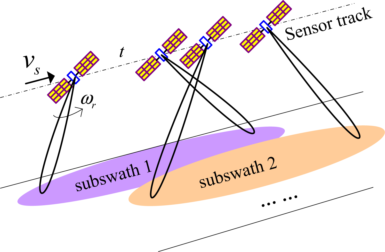
2. TOPS Imaging Mode

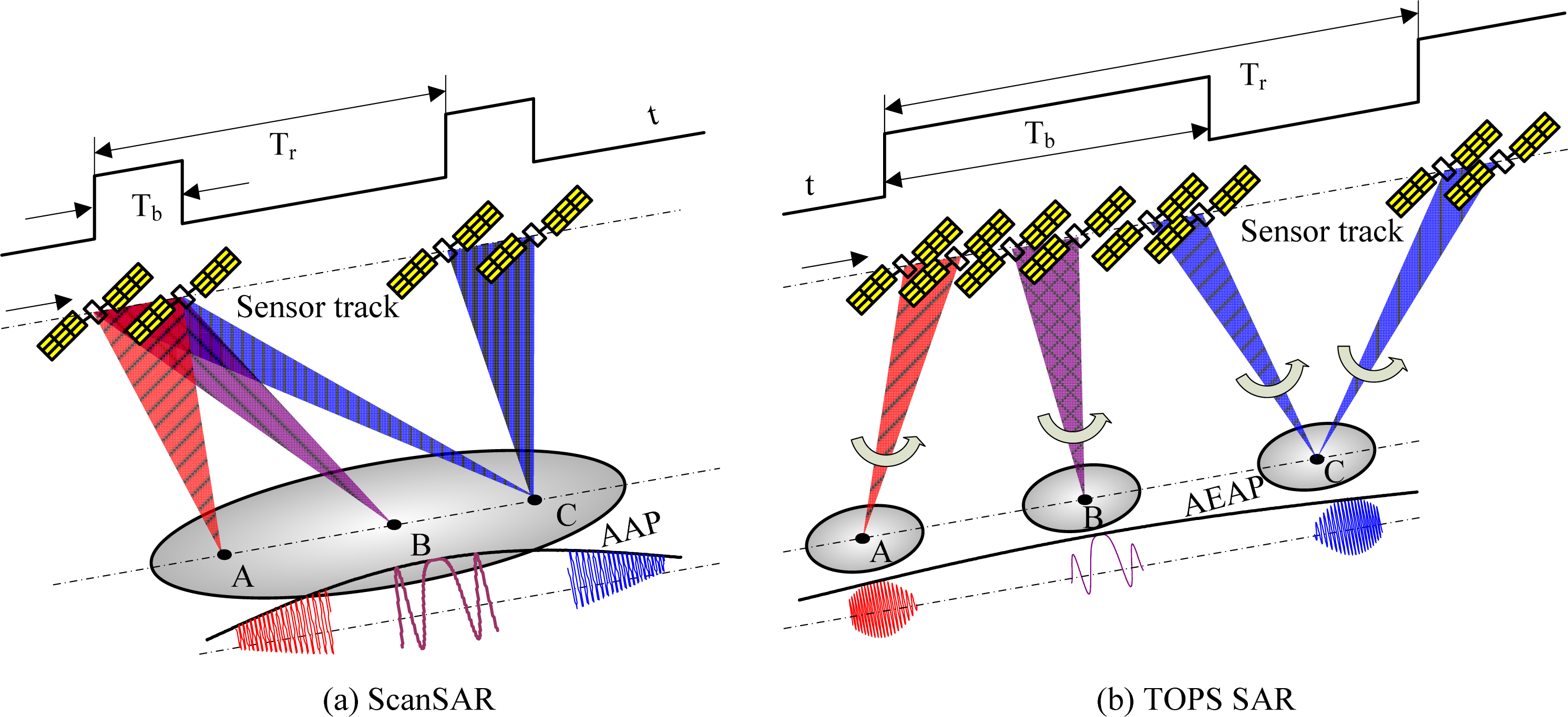
2.1. TOPS Mode Review

The TOPS mode requires the sensor antenna beam to be steered in both elevation and azimuth. In elevation, the antenna beam scans cyclically from sub-swath to sub-swath, using the burst mode similar to ScanSAR; in azimuth, the azimuth antenna beam is swept from aft to fore to shrink the target illumination time, as shown in Figure 1. In Figure 1, t defines the slow time axis (in azimuth), ω_r is the azimuth beam rotation rate, v_s is the velocity of the satellite. By taking the azimuth beam rotation into account, echoes of each target are weighted by a reduced AAP. The new AAP can be regarded as [2]:

$$G_{\mathit{TOPS}}(t)\approx G_0\cdot {\text{sinc}}^2\left[\frac{L_a}{\lambda }\frac{v_{g}t}{r}\left(1+\frac{{\omega }_{r}r}{v_g}\right)\right]$$

(1)

where G₀ is a constant representing the gain of the AAP, L_a represents the length of the azimuth antenna, v_g is the velocity of the footprint without taking azimuth beam steering into account, r is the slant range. G_TOPS(t) can be equivalent to the AAP of a fixed antenna in the classical stripmap mode, but shrunk by a factor A:

$$A(r)=1+{\omega }_{r}r/v_g$$

(2)

This factor shrinks the target illumination time and is responsible for the coarser azimuth resolution [2]. As each target experiences the completed AAP weighting in TOPS, azimuth varying system performances in conventional ScanSAR are overcome.

Since the AAP is symmetrical, the shrunk AAP can also be obtained by steering the azimuth beam from fore to aft, the same direction as the spotlight mode, but with a higher beam rotation rate. This scheme is named as the inverse TOPS (ITOPS) mode. With the same antenna, in order to obtain the same azimuth resolution, the azimuth beam rotation rate ω_ir in the ITOPS mode is expressed as follows:

$${\omega }_{\mathit{ir}}=-\left(\frac{2v_g}{r}+{\omega }_r\right)$$

(3)

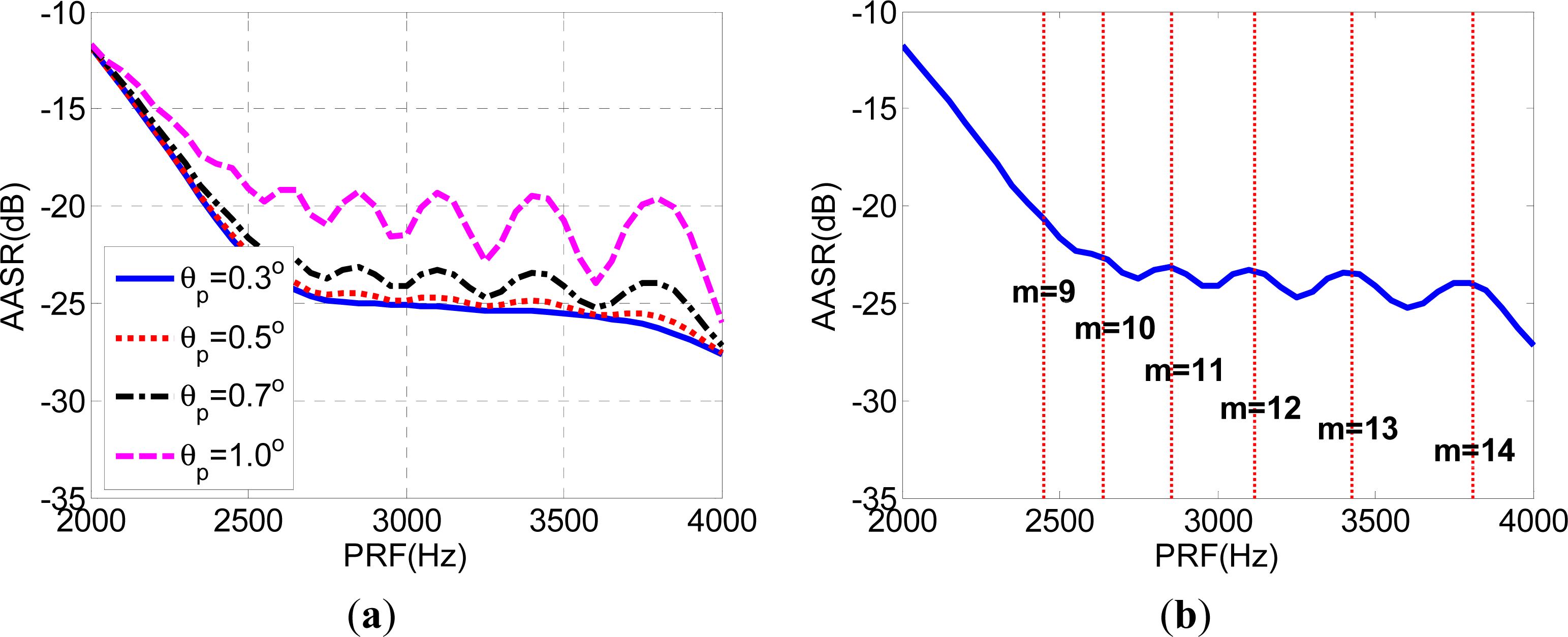
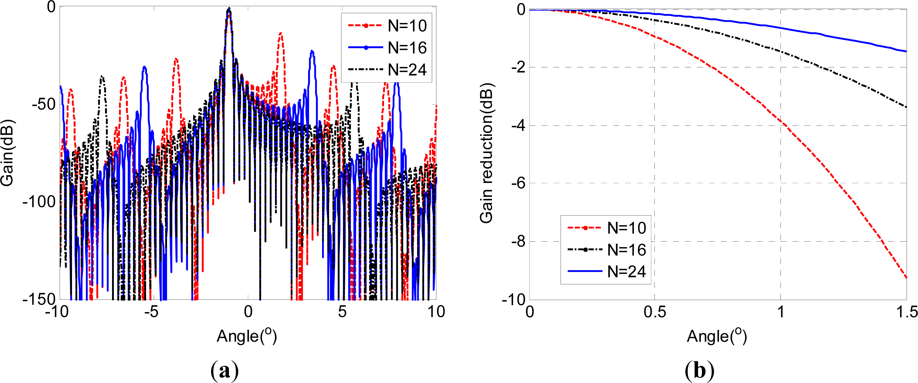
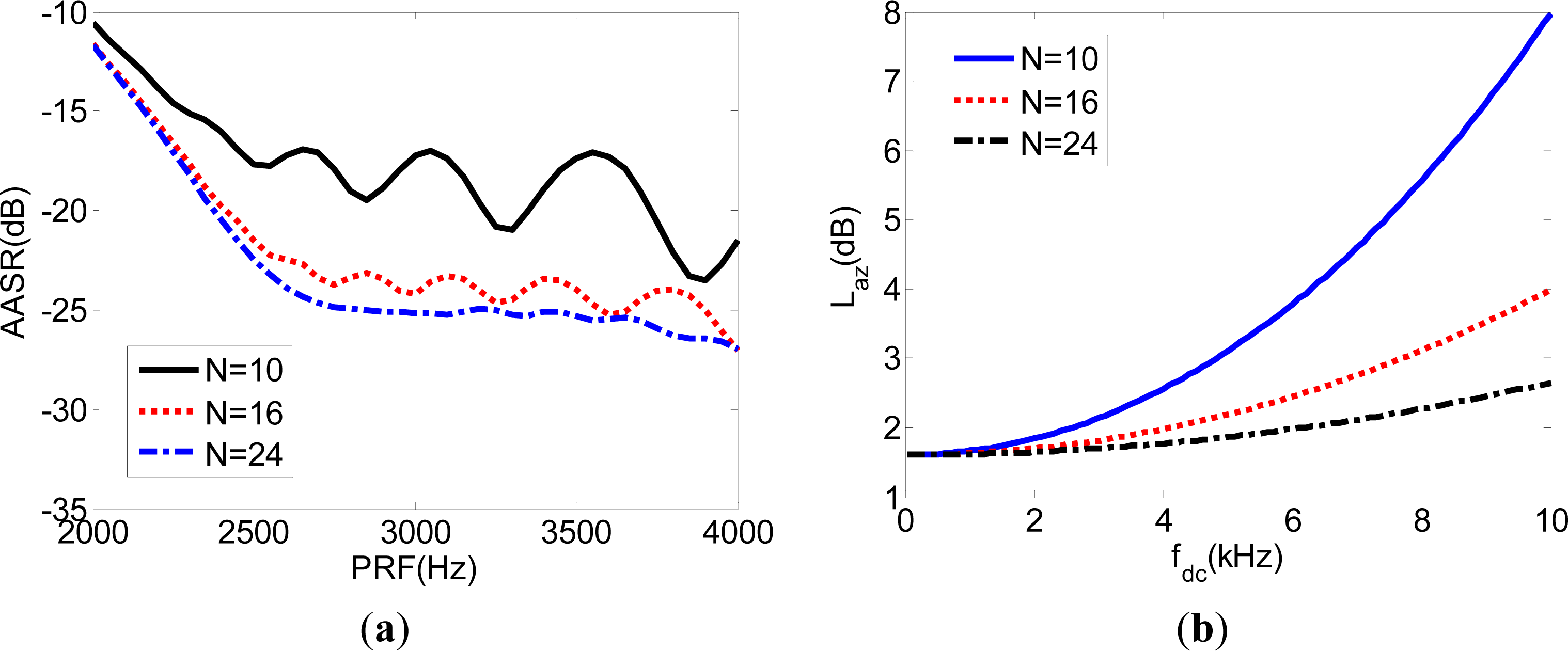
2.2. Performance Analysis in Azimuth

To implement progressive beam scanning in both azimuth and elevation, a two-dimensional (2D) planar phased array antenna is usually adopted for the spaceborne SAR missions. The two-way azimuth antenna pattern of the phased array antenna can be written as follows: [12,13]:

$$G(\theta ,t)=G_e(\theta )\cdot \left|\frac{1}{N}\sum _{k=0}^{N-1}{C}_{k,T}(t)\text{exp}\left(j\frac{2\pi k}{\lambda }{L}_{\mathit{ae}}\text{sin}\theta \right)\right|\cdot \left|\frac{1}{N}\sum _{k=0}^{N-1}{C}_{k,R}(t-\mathrm{\Delta }t)\text{exp}\left(j\frac{2\pi k}{\lambda }{L}_{ae}\text{sin}\theta \right)\right|$$

(4)

with

$$G_e(\theta )=G_0\cdot {\text{sinc}}^2\left(\frac{L_{\mathit{ae}}}{\lambda }\text{sin}\theta \right)$$

(5)

$$C_{k,T}(t)=a_{k,T}\cdot \text{exp}\left[j\frac{2\pi k}{\lambda }{L}_{\mathit{ae}}\text{sin}({\theta }_p(t))\right]$$

(6)

$$C_{k,R}(t)=a_{k,R}\cdot \text{exp}\left[j\frac{2\pi k}{\lambda }{L}_{\mathit{ae}}\text{sin}({\theta }_p(t-\mathrm{\Delta }t))\right]$$

(7)

where G_e(θ) is the antenna pattern of the antenna element, N is the number of Transmit/Receive (T/R) modules in azimuth, L_ae is the length of one antenna element, C_k,T(t) and C_k,R(t) are the excitation coefficients of the transmit and receive azimuth beam steering law, respectively, a_k,T and a_k,R are transmit and receive excitation coefficients amplitudes, respectively, Δt is the delay time for the radar echo reception, and θ_p(t) = ω_rt is the steering angle, which varies with the slow time t. Figure 2 shows the array antenna pattern, and it indicates that the grating lobe energy is increased and the main lobe gain is reduced during the antenna beam steering, when the element antenna length is longer than the wavelength. In this simulation, the frequency carrier is 9.65 GHz, and the antenna length is 6.4 m. With the increased steering angle, the grating lobes arise and the main lobe gain reduces. This shows that the azimuth beam steering capacity is limited for spaceborne SAR systems, and it is the reason for a small scalloping effect, as well as the slight azimuth variation of signal to noise (SNR) and ambiguity to signal ratio (ASR) in TOPS [14].

As azimuth burst working principles of ScanSAR and TOPS are quite different as shown in Figure 3, the two modes share different system performances. In ScanSAR, the whole synthetic aperture time of the stripmap case is divided into multiple segments to illuminate different sub-swaths; the whole synthetic aperture time of the stripmap case is compressed via steering the azimuth beam from aft to fore in TOPS. Echoes of targets at different azimuth locations are weighted by different parts of the AAP in ScanSAR, while echoes of all targets in TOPS share the complete AAP and the small difference is caused by the azimuth element antenna pattern (AEAP) as shown in Figure 3b.

The k-th grating lobe is located at angles:

$$\phi -{\phi }_0=\pm k\lambda /L_{\mathit{ae}}$$

(8)

where φ₀ is the azimuth squint angle. As signal and ambiguity energy are integrated in the focusing angular interval, the system AASR can be computed as follows [12]:

$$\text{AASR}=\frac{\sum _{m\ne 0}{\int }_{-{\vartheta }_0/2}^{{\vartheta }_0/2}{G}^2(\phi -m\cdot {\vartheta }_{\mathit{amb}})d\phi }{{\int }_{-{\vartheta }_0/2}^{{\vartheta }_0/2}{G}^2(\phi )d\phi }$$

(9)

where ϑ₀ is the focusing angular interval, ϑ_amb is the interval angle between two ambiguity directions and is described as:

$${\vartheta }_{\mathit{amb}}=\frac{\lambda \cdot \text{PRF}}{2v_s}$$

(10)

The main azimuth ambiguity energy will be introduced by the grating lobe and the AASR will become worse, if the system PRF is selected as follows:

$$\text{PRF}=\frac{2\mathit{kv}}{m{L}_{\mathit{ae}}},\hspace{0.17em}\hspace{0.17em}\hspace{0.17em}\hspace{0.17em}\hspace{0.17em}\hspace{0.17em}\hspace{0.17em}\hspace{0.17em}k,m\in \{1,2,3,\dots ,N\}$$

(11)

Since the first pair of grating lobes has the highest energy power, the case of k = 1 should be considered during the TOPS mode system design. Figure 4 shows simulation results of AASR varying with the PRF, the squint angle of Figure 4b is 0.7° and the azimuth antenna is 6.4 m consisting of 16 elements. For the increased squint angle grating lobes arise, and Figure 4 illustrates their impact on the AASR.

In addition to the impact of grating lobes on the AASR, the effect of main lobe gain reduction on the SNR should be considered during the system design. The effect can be expressed by the azimuth loss L_az given as:

$$L_{\mathit{az}}=\frac{{\int }_{-B_d/2+f_{\mathit{DC}}}^{B_d/2+f_{\mathit{DC}}}{\left|H_p(f_a)\right|}^2{\mathit{df}}_a}{{\int }_{-B_d/2+f_{\mathit{DC}}}^{B_d/2+f_{\mathit{DC}}}{\left|G_a(f_a)\right|}^2\cdot {\left|H_p(f_a)\right|}^2{\mathit{df}}_a}$$

(12)

where H_p(f_a) is the transfer function of the azimuth processing filter, B_d is the target Doppler bandwidth, f_DC is the target Doppler centroid, G_a(f_a) is the joint Tx-Rx azimuth antenna pattern function which is weighting the Doppler spectrum.

From Equations (9) and (12), it can be seen that the AAP will affect the system performances AASR and the azimuth loss, and Figure 5 demonstrates this effect. If more antenna elements are adopted for a fixed antenna length, the effect on grating lobes and main lobe reduction will be reduced. This results in a better system performance.

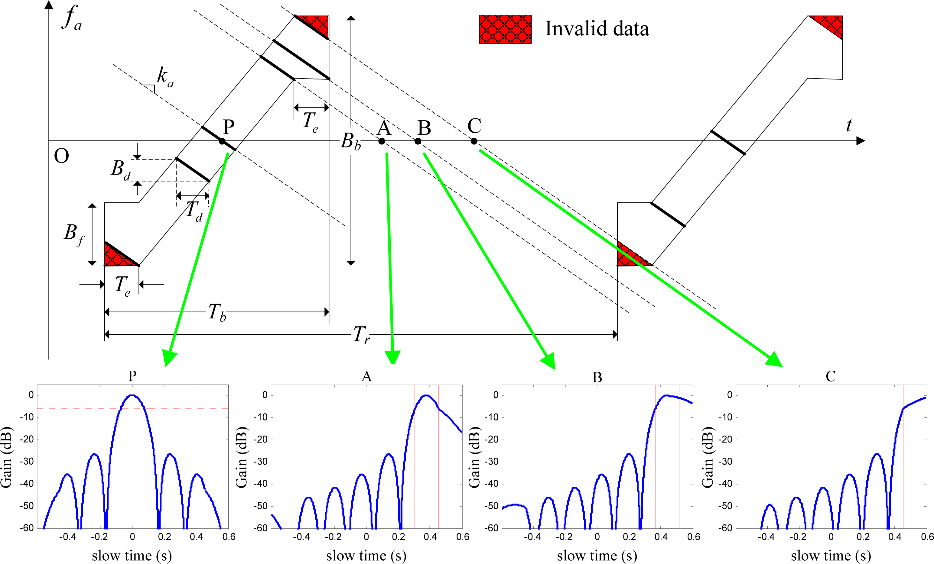
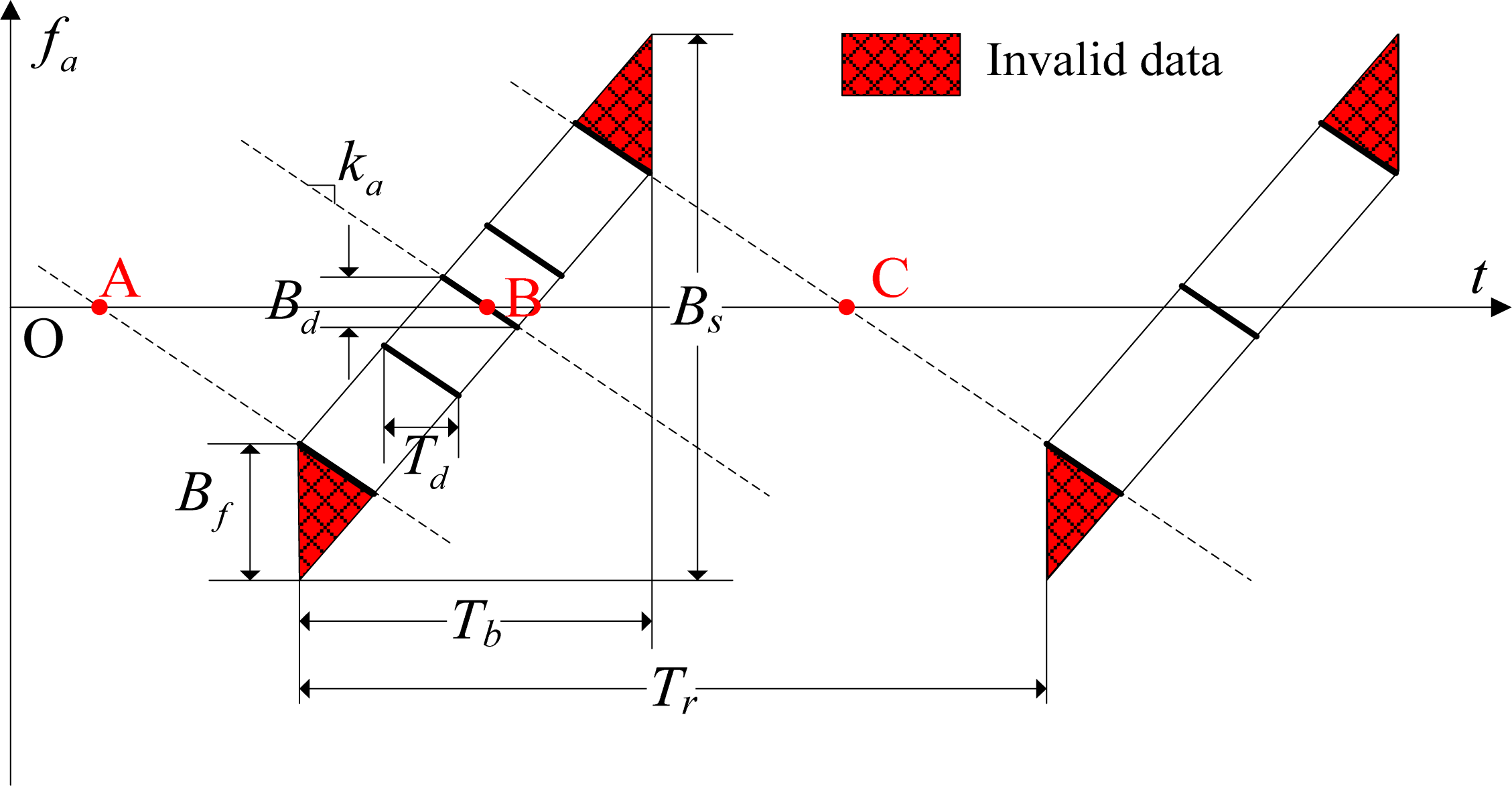
2.3. Timeline Design in TOPS

For burst imaging schemes, different sub-swaths are periodically illuminated in elevation, and the timeline design becomes very important to keep the imaged area continuous in both azimuth and elevation. After computing the azimuth beam steering rate in the i-th sub-swath, the TOPS timeline could be derived. The constraint of the TOPS timeline results in a set of n linear equations as follows [6,9]:

$$({\omega }_{r\_i}{T}_{b\_i}-{\vartheta }_0)R_i+v_g{T}_{b\_i}=(1+\epsilon )v_g\sum _i^N{T}_{b\_i}=(1+\epsilon )v_g{T}_r$$

(13)

where T_{b_i} is the burst duration of the i-th sub-swath, ϑ₀ is the azimuth beam interval exploited for focusing, R_i is the closest slant range, ε is the overlap ratio between two adjacent imaged areas in azimuth, and T_r is the cycle time. Figure 6 shows the proper TOPS timeline in the azimuth time-frequency diagram for keeping the imaged area continuous in azimuth, while A and C are targets at the edge of the imaged area of a burst. In Figure 6, k_a is the azimuth signal modulation rate, T_d is the target dwell time, B_f, B_d and B_s are bandwidths of the azimuth beam, a point target and the burst, respectively. The shadow areas of the TOPS time-frequency diagram (TFD) represent raw data of partly illuminated targets, which are usually considered as invalid data and will be canceled during TOPS SAR focusing.

According to Equation (13) and the system parameters listed in

Table 1. Simulation parameters.

Parameters	Value
Height of satellite H (km)	630
Satellite velocity vs (m/s)	7,554
Carrier frequency f0 (GHz)	9.65
Look angle (°)	15∼45
Transmitted pulse width τp (μs)	40
Azimuth antenna length La (m)	6.4
Elevation antenna height Lr (m)	0.60
Number of Transmit/Receive (T/R) modules	16 × 20
Transmit peak power (W)	2,560
Swath width (km)	≥120
Azimuth resolution ρaz (m)	≤15
Azimuth Ambiguity to Signal Ratio (AASR) (dB)	≤−20
Overlap ratio	5%

, Figure 7 shows the relationship between the cycle time and the azimuth resolution. It can be seen that a better azimuth resolution needs a larger cycle time, and this indicates that a stronger azimuth beam steering capability is required for a better azimuth resolution in TOPS. However, the azimuth beam steering capability is very limited in recent spaceborne SAR systems, e.g., ±0.75° in the TerraSAR-X and ±0.7° in the Sentinel-1 case.

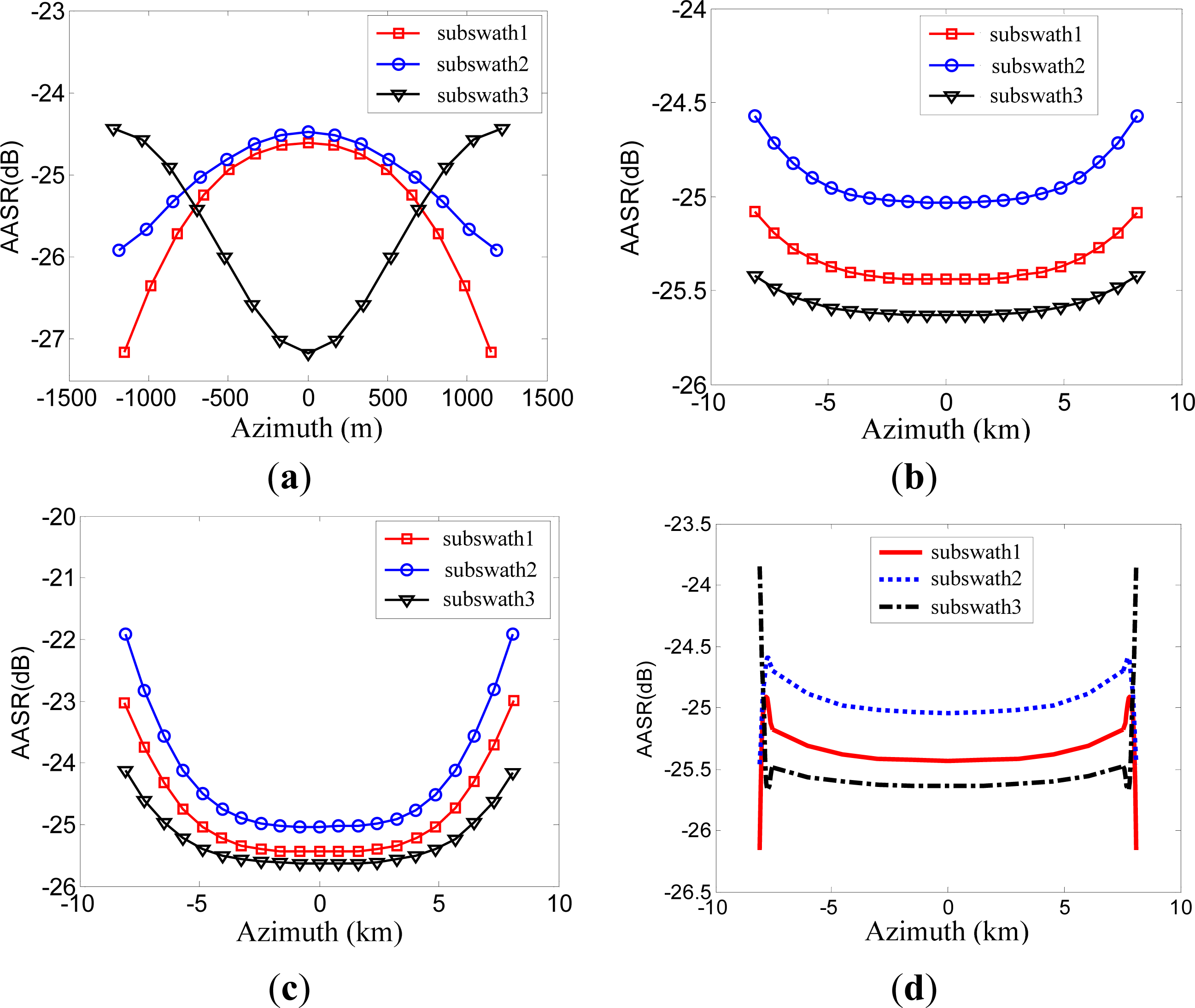
3. ETOPS Imaging Mode

To improve the azimuth resolution for spaceborne SAR systems with a limited azimuth beam steering capability, a new burst imaging mode named ETOPS is proposed. The only difference between TOPS and ETOPS modes is that two short extended burst durations are added before and after the conventional TOPS burst duration, respectively. During the extended burst duration, the azimuth beam pointing direction is kept fixed at the center steering angles. The extended burst duration T_e is computed as follows:

$$T_e=\frac{B_d}{\left|k_a\right|}=\frac{{\rho }_a}{\left|k_a\right|v_g}$$

(14)

where ρ_a is the desired azimuth resolution.

Figure 8 demonstrates the ETOPS timeline in the azimuth time-frequency diagram to keep the imaged area continuous in azimuth, and the bottom of Figure 8 shows AAPs seen by point targets with different azimuth positions. The effective azimuth extension L_{eff_ETOPS} of the imaged area for a burst in ETOPS can be expressed as follows:

$$L_{\mathit{eff}\_\mathit{ETOPS}}\approx ({\omega }_{r}R+v_g)\cdot (T_b-2T_e)+{\vartheta }_{0}R=({\omega }_{r}R+v_g)\cdot T_b-{\vartheta }_{0}R$$

(15)

Therefore, the constraint of the ETOPS timeline results in a set of n linear equations as follows:

$$({\omega }_{r\_i}{R}_i+v_g)\cdot T_{b\_i}-{\vartheta }_0{R}_i=(1+\epsilon )v_g\sum _i^N{T}_{b\_i}=(1+\epsilon )v_g{T}_r$$

(16)

Compared with Equation (13), the cycle time T_r of the ETOPS mode is the same as the one of the TOPS mode. Different from the conventional TOPS mode, the whole burst duration T_b includes three parts in the ETOPS mode as shown in Figure 8. The azimuth time interval for azimuth beam steering is just T_b − 2·T_e. Moreover, the azimuth beam is not steered at the burst edges in ETOPS, and the SAR system is working in the squinted stripmap mode. This explains why a smaller azimuth beam scanning capability is required in ETOPS for the same azimuth resolution and range swath width in TOPS.

In Figure 8, point targets A, B and C could not be fully imaged in the conventional TOPS mode, while they would be focused well in ETOPS with the same azimuth beam steering capability. Furthermore, compared to Figure 6, the ratio between the raw data of partly illuminated targets and the whole raw data in ETOPS is obviously lower than the ratio in TOPS. With parameters of sub-swath 1 in TOPS and ETOPS listed in

Table 2. Parameters of different sub-swaths in ScanSAR.

Sub-Swath	Sub-Swath-1	Sub-Swath-2	Sub-Swath-3
Parameters
Burst duration (s)	0.103	0.106	0.109
Echoes per burst	340	297	385
Target dwell time Td (s)	0.103	0.106	0.109
Target bandwidth Bd (Hz)	489.78	489.62	489.58
Burst bandwidth Bb (kHz)	2.088	2.088	2.088
Azimuth extension Leff (km)	2.296	2.365	2.434
Azimuth resolution ρa (m)	14	14	14

Table 3. Parameters of different sub-swaths in Terrain Observation by Progressive Scans (TOPS).

Sub-Swath	Sub-Swath-1	Sub-Swath-2	Sub-Swath-3
Parameters
Burst duration Tb (s)	0.748	0.751	0.755
Echoes per burst	2474	2110	2671
Target dwell time Td (s)	0.117	0.120	0.124
Beam steering rate ωr (°/s)	1.550	1.505	1.462
Max steering angle θmax(°)	0.579	0.565	0.552
Target bandwidth Bd (Hz)	571.4	571.2	571.2
Burst bandwidth Bb (kHz)	11.009	10.787	10.579
Azimuth extension Leff (km)	16.222	16.217	16.216
Azimuth resolution ρa (m)	12	12	12

Table 4. Parameters of different sub-swaths in inverse TOPS (ITOPS).

Sub-Swath	Sub-Swath-1	Sub-Swath-2	Sub-Swath-3
Parameters
Burst duration Tb (s)	0.748	0.751	0.755
Echoes per burst	2474	2110	2671
Target dwell time Td (s)	0.117	0.120	0.124
Beam steering rate ωr (°/s)	2.677	2.599	2.526
Max steering angle θmax (°)	1.001	0.976	0.953
Target bandwidth Bd (Hz)	571.4	571.2	571.2
Burst bandwidth Bb (kHz)	17.496	17.113	16.754
Azimuth extension Leff (km)	16.222	16.217	16.216
Azimuth resolution ρa (m)	12	12	12

and

Table 5. Parameters of different sub-swaths in Extended Terrain Observation by Progressive Scans (ETOPS).

Sub-Swath	Sub-Swath-1	Sub-Swath-2	Sub-Swath-3
Parameters
Burst duration Tb (s)	0.748	0.751	0.755
Echoes per burst	2474	2110	2671
Extended burst duration Te (s)	0.117	0.120	0.124
Target dwell time Td (s)	0.117	0.120	0.124
Beam steering rate ωr (°/s)	1.550	1.505	1.462
Max steering angle θmax (°)	0.398	0.385	0.371
Target bandwidth Bd (Hz)	571.4	571.2	571.2
Burst bandwidth Bb (kHz)	9.123	8.888	8.652
Azimuth extension Leff (km)	16.222	16.217	16.216
Azimuth resolution ρa (m)	12	12	12

, the ratio in TOPS is 0.156, while the ratio in ETOPS is 0.063. The bottom of Figure 8 shows the resulting antenna pattern as seen by the point targets at the different azimuth locations.

The proposed ETOPS mode in this paper is inspired from another extended TOPS mode named as TOPSPOT [13]. The TOPSPOT is actually a combination of a TOPS SAR and a SPOTSAR scanning, while the proposed ETOPS mode is actually a combination of a TOPS SAR mode and a stripmap mode. The same principle of the TOPSPOT mode and the ETOPS mode is that two short extended burst durations are added before and after the conventional TOPS SAR burst duration. The major difference between the TOPSPOT mode and the ETOPS mode is that the SAR system works in the spotlight mode and the azimuth beam requires being steered during the whole extended burst duration in the TOPSPOT mode, while the SAR system works in the stripmap mode and the azimuth beam pointing direction is fixed during the whole extended burst duration in the ETOPS mode. As a result, the AAP illumination of the ETOPS mode for different targets is different from the TOPSPOT mode as shown in Figure 8. Compared with the TOPSPOT mode, targets at the edge of the imaged area in azimuth will be better illuminated.

4. System Design

To validate the proposed imaging mode for wide swath coverage, four imaging modes for wide swath coverage with the same system parameters are first designed and their corresponding system performances are analyzed and compared. The major system parameters and system performance requirements are listed in Table 1.

First, a timing analysis is performed. The length of the whole swath consisting of three sub-swaths is 130 km as shown in Figure 9. With the same timing diagram selection result and system parameters listed in Table 1, four wide width imaging modes (ScanSAR, TOPS, ITOPS and ETOPS) are designed. The parameters of the different sub-swaths for the different modes are computed and summarized in Tables 2 and 5.

With the same system parameters, the obtained azimuth resolution is 14 m in ScanSAR, while the obtained azimuth resolution of the other modes is 12 m. This phenomenon is caused by different imaging principles to keep the imaged area continuous in azimuth. For the same desired azimuth resolution, the maximum azimuth steering angle in TOPS, ITOPS and ETOPS are 0.579°, 1.001° and 0.398°, respectively, and the ETOPS mode requires a lower azimuth beam steering angle than the other two modes.

Figure 10 shows the azimuth ambiguity to signal ratio (AASR) of the different imaging modes a function of the target along-track position. The azimuth variant AASR is the most obvious in ScanSAR, since echoes of different targets are weighted by different parts of the AAP depending on the target’s azimuth locations. The slight AASR variation along the azimuth direction in TOPS and ITOPS is caused by the increased grating lobes and the main lobe reduction during azimuth beam steering. This effect is more obvious in ITOPS than in TOPS, since a higher steering angle is required for a desired azimuth resolution. As the azimuth beam pointing direction is fixed during the extended burst duration in ETOPS, the azimuth variant AASR is obvious at the edge of the imaged area in azimuth, but it is less obvious than ScanSAR as shown in Figure 10d.

Noise-equivalent sigma zero (NESZ) is also a function of the target along-track position. In ScanSAR, this variation exceeds 3 dB as shown in Figure 11a, since echoes of targets with different azimuth locations are weighted by different parts of the AAP. This variation is less than 0.3 dB in TOPS and less than 1.2 dB in ITOPS, since it is caused by the antenna gain reduction during azimuth beam steering. In ETOPS, the NESZ variation in azimuth is about 2 dB and better than that of ScanSAR.

Performance analysis results as shown in Figures 10 and 11 validate the proposed ETOPS mode. The azimuth performance variation in ETOPS is better than in ScanSAR. Furthermore, for the same azimuth resolution, the ETOPS mode requires a smaller azimuth beam steering angle than the TOPS and ITOPS modes, which also means that a better azimuth resolution could be obtained in ETOPS for a limited azimuth beam steering capability.

5. Conclusions

Burst imaging schemes are usually adopted for wide swath coverage. This paper proposes a new burst imaging scheme named ETOPS. Performance (AASR and NESZ) of the ETOPS are better than ScanSAR, but little worse than the TOPS mode. However, with a limited azimuth beam scanning capability, the ETOPS mode could implement a better azimuth resolution than the TOPS mode. Furthermore, the ratio between the raw data of partly illuminated targets and the whole raw data in ETOPS is obviously lower than the ratio in TOPS. Four different burst imaging modes for wide swath coverage have been designed with the same system parameters, and their corresponding performances are analyzed and compared. Simulation results validate the proposed ETOPS mode for wide swath coverage.

References

1. Currie, A.; Brown, M.A. Wide-swath SA. Proc. Inst. Elect. Eng. F 1992, 139, 123–135. [Google Scholar]
2. Moore, R.K.; Claassen, J.P.; Lin, Y.H. Scanning spaceborne synthetic aperture radar with integrated radiometer. IEEE Trans. Aerosp. Electron. Syst 1981, 17, 410–420. [Google Scholar]
3. Guarnieri, A.M.; Prati, C. ScanSAR focussing and interferometry. IEEE Trans. Geosci. Remote Sens 1996, 34, 1029–1038. [Google Scholar]
4. Holzner, J.; Bamler, R. Burst-Mode and ScanSAR Interferometry. IEEE Trans. Geosci. Remote Sens 2002, 40, 1917–1934. [Google Scholar]
5. Rosen, P.; Hensley, S.; Joughin, I.R.; Li, F.K.; Madsen, S.; Rodríguez, E.; Goldstein, R. Synthetic aperture radar interferometry. Proc. IEEE 2000, 88, 333–382. [Google Scholar]
6. Zan, F.D.; Guarnieri, A.M. TOPSAR: Terrain observation by progressive scans. IEEE Trans. Geosci. Remote Sens 2006, 44, 2352–2360. [Google Scholar]
7. Xu, W.; Huang, P.-P.; Deng, Y.-K. TOPSAR data focusing based on azimuth scaling preprocessing. Adv. Space Res 2011, 48, 270–277. [Google Scholar]
8. Xu, W.; Huang, P.-P.; Deng, Y.-K.; Sun, J.-T.; Shang, X.-Q. An efficient imaging approach with scaling factors for TOPS mode SAR data focusing. IEEE Geosci. Remote Sens. Lett 2011, 8, 929–933. [Google Scholar]
9. Meta, A.; Mittermayer, J.; Prats, P.; Scheiber, R.; Steinbrecher, U. TOPS imaging with TerraSAR-X: Mode design and perfomance analysis. IEEE Trans. Geosci. Remote Sens 2010, 48, 759–769. [Google Scholar]
10. Meta, A.; Prats, P.; Steinbrecher, U.; Mittermayer, J.; Scheiber, R. TerraSAR-X TOPS and ScanSAR Comparison. Proceedings of the 7th European Conference on Synthetic Aperture Radar (EUSAR), Friedrichshafen, Germany, 2–5 June 2008.
11. Attema, E.; Davidson, M.; Floury, N.; Levrini, G.; Rosich, B.; Rommen, B.; Snoeij, P. Sentinel-1 ESA’s New European Radar Observatory. Proceedings of the 7th European Conference on Synthetic Aperture Radar (EUSAR), Friedrichshafen, Germany, 2–5 June 2008; 2, pp. 179–182.
12. Xu, W.; Deng, Y.K. Investigation on electronic azimuth beam steering in the spaceborne SAR imaging modes. J. Electromagn. Wave. Appl 2011, 25, 2076–2088. [Google Scholar]
13. D’Aria, D.; de Zan, F.; Giudici, D.; Guarnieri, A.M.; Rocca, F. Burst-mode SARs for wide-swath surveys. Can. J. Remote Sens 2007, 33, 27–38. [Google Scholar]
14. Wollstadt, S.; Prats, P.; Bachmann, M.; Mittermayer, J.; Scheiber, R. Scalloping correction in TOPS imaging mode SAR data. IEEE Geosci. Remote Sens. Lett 2012, 9, 614–618. [Google Scholar]
Figure 1. Terrain Observation by Progressive Scans (TOPS) mode acquisition geometry.
Remotesensing 06 00801f1
Figure 2. Antenna beam steering. (a) Grating lobes; (b) Main lobe reduction.
Remotesensing 06 00801f2
Figure 3. Different azimuth burst imaging schemes in ScanSAR and TOPS. (a) ScanSAR; (b) TOPS SAR. (SAR = synthetic aperture radar)
Remotesensing 06 00801f3
Figure 4. Azimuth ambiguity to signal ratio (AASR) varying with the pulse repetition frequency (PRF). (a) With different steering angles; (b) With a steering angle of 0.7°.
Remotesensing 06 00801f4
Figure 5. The impact of the azimuth antenna pattern (AAP) on the AASR and the azimuth loss Laz. (a) AASR; (b) Azimuth loss Laz.
Remotesensing 06 00801f5
Figure 6. The TOPS timeline in the azimuth time-frequency diagram.
Remotesensing 06 00801f6
Figure 7. The relationship between cycle time and azimuth resolution.
Remotesensing 06 00801f7
Figure 8. The Extended Terrain Observation by Progressive Scans (ETOPS) timeline in the azimuth time-frequency diagram.
Remotesensing 06 00801f8
Figure 9. The timing diagram for wide-swath imaging with three-sub-swaths according to Table 1.
Remotesensing 06 00801f9
Figure 10. AASR of different imaging modes. (a) ScanSAR; (b) TOPS; (c) ITOPS; (d) ETOPS.
Remotesensing 06 00801f10
Figure 11. Noise-equivalent sigma zero (NESZ) of different imaging modes. (a) ScanSAR; (b) TOPS; (c) ITOPS; (d) ETOPS.
Remotesensing 06 00801f11