Cloud and Cloud-Shadow Detection in SPOT5 HRG Imagery with Automated Morphological Feature Extraction

Abstract

Detecting clouds in satellite imagery is becoming more important with increasing data availability, however many earth observation sensors are not designed for this task. In Satellite pour l’Observation de la Terre 5 (SPOT5) High Resolution Geometrical (HRG) imagery, the reflectance properties of clouds are very similar to common features on the earth’s surface, in the four available bands (green, red, near-infrared and shortwave-infrared). The method presented here, called SPOTCASM (SPOT cloud and shadow masking), deals with this problem by using a series of novel image processing steps, and is the first cloud masking method to be developed specifically for SPOT5 HRG imagery. It firstly detects marker pixels using image specific threshold values, and secondly grows segments from these markers using the watershed-from-markers transform. The threshold values are defined as lines in a 2-dimensional histogram of the image surface reflectance values, calculated from two bands. Sun and satellite angles, and the similarity between the area of cloud and shadow objects are used to test their validity. SPOTCASM was tested on an archive of 313 cloudy images from across New South Wales (NSW), Australia, with 95% of images having an overall accuracy greater than 85%. Commission errors due to false clouds (such as highly reflective ground), and false shadows (such as a dark water body) can be high, as can omission errors due to thin cloud that is very similar to the underlying ground surface. These errors can be quickly reduced through manual editing, which is the current method being employed in the operational environment in which SPOTCASM is implemented. The method is being used to mask clouds and shadows from an expanding archive of imagery across NSW, facilitating environmental change detection.

1. Introduction

Clouds and their shadows are often a significant problem when conducting remote sensing of the earth’s surface as they can locally obscure surface features and alter reflectance. Their masking, and exclusion from analysis, is an important pre-processing step in many applications. Automating the masking is especially important in multi-temporal studies over large areas where hundreds or thousands of images require processing. The research into cloud masking presented here was conducted to facilitate large area vegetation monitoring by the Office of Environment and Heritage (OEH) in New South Wales (NSW), Australia. OEH has been monitoring woody vegetation change, such as tree removal, with Satellite pour l’Observation de la Terre 5 (SPOT5) High Resolution Geometrical (HRG) data for a number of years, and now has over 2,000 SPOT5 HRG images. At the time of this research, the archive contained 313 SPOT5 HRG images contaminated by cloud acquired between 2004 and 2012. All images are assessed for cloud contamination by a visual quality control process, and their locations are shown on Figure 1.

Some recently developed automated methods for cloud and shadow masking of Landsat-5 Thematic Mapper (TM) and Landsat-7 Enhanced Thematic Mapper (ETM+) imagery have greatly facilitated large area studies [1,2]. As the spectral and spatial resolution of a sensor affects the methods employed to detect clouds, the existing methods described above cannot be employed for SPOT5 HRG data. For example, methods that exploit clouds as being highly reflective in visible wavelengths and with lower temperatures than the ground surface [1,3], cannot be used on data from sensors that do not measure infrared (IR) wavelengths emitted by the earth’s surface. Spatial resolution is also important in detecting clouds, as highly reflective surface features that have similar spectral characteristics to clouds become more common as pixel size is reduced. For example, statistical classification methods that work well for images with 1–3 km pixels [4], and even 250 m pixels [5,6] produce poor results for images with 10 m pixels, as at this higher spatial resolution many small features such as bare ground and buildings can all have spectral reflectance values indistinguishable from cloud.

SPOT5 HRG data has a 10 m pixel size that allows it to be used for environmental monitoring of features too small to be visible in the commonly used 30 m Landsat TM/ETM+ data. It also lacks a thermal IR band, having only four spectral bands in the green (0.49–0.61 μm), red (0.61–0.68 μm), near-IR (NIR) (0.78–0.89 μm) and shortwave-IR (SWIR) (1.58–1.75 μm). It is similar to SPOT4 High Resolution Visible IR (HRVIR) imagery, for which two novel cloud and cloud-shadow masking methods have been developed. The first exploits the parallax between panchromatic and multispectral sensors on the satellites but was difficult to implement and did not significantly improve on simpler spectral-based classifications [7]. The second, developed by le Hégarat-Mascle and André [8], identifies cloud and cloud shadows by identifying the relationships between the two objects. This method achieved good results when applied to 39 SPOT4 HRVIR images from semi-arid West Africa, with a median commission and omission error rate for cloud pixels of 8%.

The research presented here has two aims. The first was to review the existing approach of le Hégarat-Mascle and André [8], applied to SPOT5 HRG imagery in NSW, Australia, to identify its limitations. The second aim was to adapt this method and develop a new method, to be used in an operational environmental monitoring program.

2. Existing Cloud Masking Methods for SPOT Imagery

The le Hégarat-Mascle and André [8] method involved the following steps: identifying potential clouds with an image-specific threshold-line on a 2-dimensional scatter-plot of pixels (using the green and SWIR bands); identifying potential shadows as dark areas in the SWIR band at the correct angle from the clouds; and, discarding cloud and shadow pairs if they had significantly different shapes, based on the area of overlap between a translated cloud and its assumed shadow. Comparing results with manual classifications gave both a producer’s and user’s accuracy for cloud of 92% [9]. While the method performed well for the 20 m resolution SPOT4 HRVIR images from West Africa, our trial of the method on 10 m resolution SPOT5 HRG images over NSW, Australia, highlighted several problems.

Firstly, water bodies and snow were found to contain pixels that were confused with cloud, as they had green and SWIR reflectance properties that placed them above the cloud threshold line. Water pixels were also confused with cloud-shadows, as they often had lower SWIR reflectance than cloud-shadows. An example of the similarity between water and cloud-shadow pixels for image 8 is shown in Figure 2. If these water pixels are not removed, it is possible to validate a false cloud by a false shadow. In particular, small water bodies like farm dams were often detected in the expected shadow positions

Secondly, many high reflectance features, such as buildings, were being confused as clouds. Features such as buildings, bare-ground and rock that may only be 1–2 pixels in size were above the cloud threshold line. An example of the similarity between buildings and cloud pixels for image 8 is shown in Figure 2. Further complications arose when the expected shadow position was covered with other small false positive clouds.

Thirdly, areas of high topographic relief caused problems as topographic shadows were identified as cloud-shadows, and the distorted shape of cloud-shadows in high relief areas does not match the cloud shape. While topographic shadows are spectrally identical to cloud-shadows and will always be a problem for cloud-shadow masking methods, the way cloud-shadows are found needed altering for images with high topographic relief. In particular, searching for the darkest object as a shadow can preferentially find a topographic shadow, even when a cloud-shadow clearly exists. Also, the le Hégarat-Mascle and André [8] method used hysteresis thresholding to grow cloud-shadow segments from the darkest area, which can result in cloud-shadows growing into topographic shadows.

3. Method

The cloud and cloud-shadow masking method described here, called SPOTCASM (SPOT Cloud and Shadow Masking), is based on the method of le Hégarat-Mascle and André [8], but also includes the following new components: masking water bodies from images before searching for clouds and shadows; limiting the shadow search area by assuming that clouds are at similar heights; filtering possible clouds to remove very small objects; and, using the watershed-from-markers transform to grow cloud and cloud-shadow segments from marker pixels [10]. These last two ideas use morphological image processing techniques often used for extracting features from images [11]. Parts of the le Hégarat-Mascle and André [8] method that were adapted include: identifying linear threshold lines in 2-dimensional space based on the distribution of pixels; limiting the search for cloud-shadows to the appropriate direction from possible clouds; and, comparing the possible cloud and shadow pairs to determine which are valid.

SPOTCASM is implemented with a script written in the Python programming language, using functions from the standard Python library [12,13], as well as from the following freely-available open-source Python modules: Numpy [14], Scipy [15], GDAL [16], Pymorph [11,17] and Mahotas [18]. The program is open-source and available online under the GNU General Public License, Version 3 [19]. As many components of the method make use of morphological image processing, it is appropriate to describe this first.

3.1. Morphological Image Processing

Morphological image processing is based on exploiting the geometric structures within images, and can be used to design algorithms for automatic object recognition or feature extraction. The following section describes some of the fundamental components of the technique that are used in the new cloud and shadow masking method, summarized from the work of Dougherty and Lotufu (2003) [11]. The fundamental idea of morphological image processing is erosion, which is to probe an image with a structuring element, and observe where the element fits and where it does not (a structuring element, similar to a filter kernel, is defined by its size, shape, pixel values, and the position of its origin). This concept is straightforward for binary images, where a structuring element can fit or not fit at different pixel locations, resulting in the features in an image shrinking, or being eroded. Applying the concept to grayscale images is more complex, but it can be simplified if only flat (binary) structuring elements are considered, resulting in the erosion of an image by the structuring element g being the same as applying a moving-minimum filter with a kernel g: it removes isolated pixels with large values (bright pixels) and erodes image features that are collections of bright pixels. The opposite of morphological erosion is dilation, which is the same as a moving-maximum filter, and has the effect of removing isolated pixels with small values (dark pixels) and erodes image features that are collections of dark pixels.

Many useful morphological image processing methods have been developed by combining erosion and dilation. For example, morphological opening (erosion followed by dilation) removes bright features smaller than the structuring element, while maintaining bright features larger than the structuring element. Morphological closing (dilation followed by erosion) removes small dark features while maintaining larger dark features. If an image contains noise consisting of both bright and dark features, they can be removed by applying an opening followed by a closing. Furthermore, if the noisy features are a mixture of different spatial sizes, it can be useful to repeat the opening-closing with structuring elements of increasing size, termed an alternating sequential filter (ASF). This removes high frequencies within image objects that are larger than the largest structuring element used, while maintaining the edges of these objects, and is used in the SPOTCASM method.

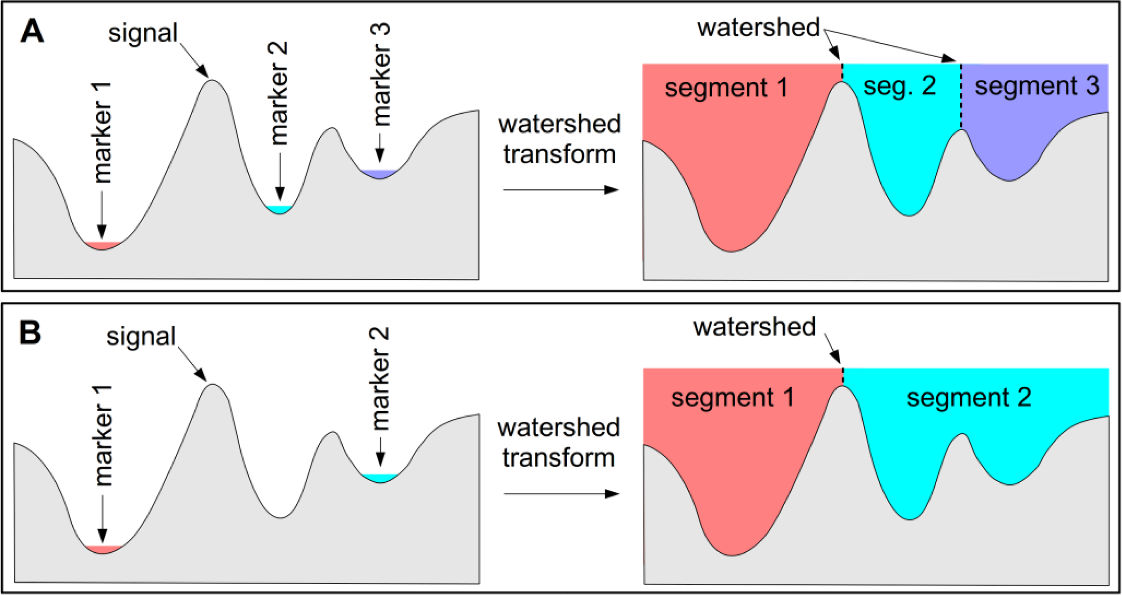
The watershed transform is a more complex morphological technique for image segmentation or feature extraction that can also be used for identifying peaks and troughs in one-dimensional signals. It is best explained by considering the flooding simulation of a signal, where holes are punched in each minima or trough and the signal is flooded by gradually immersing it in water (Figure 3A). The watershed lines are the points at which the waters from different basins meet. When applying the watershed transform to an image it is common to apply it to the morphological gradient (dilation minus erosion) of the image, which is a form of edge detection used to define potential watershed lines between image features. When the morphological gradient of an image is viewed as a topographic surface flooded from the minima, an image is commonly over-segmented due to minima from image noise. While this can be somewhat improved through filtering, the best improvement is gained when a set of minima are selected to act as markers. Applying the watershed-from-markers transform greatly reduces over-segmentation, though it makes it necessary to identify marker pixels for each image object (Figure 3B). In the case of feature extraction, it is necessary to identify internal markers for the features, and also external markers for the background pixels against which the features sit. The watershed-from-markers transform is used in several steps of the SPOTCASM method.

3.2. Image Selection and Pre-Processing

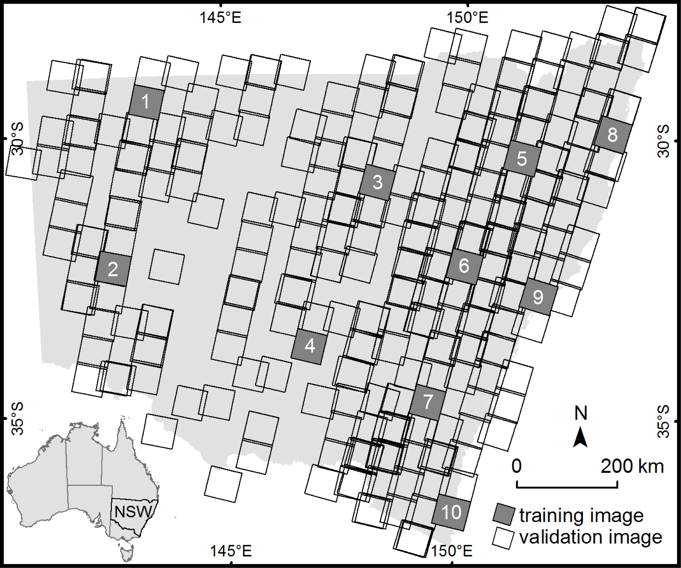
SPOTCASM was developed primarily for the OEH SPOT5 HRG image archive. Over 300 SPOT5 HRG images are required to cover NSW, an area of over 800,000 km² that has a large variety of landcover types including subtropical rainforest, alpine herbfields and arid shrublands. Acquisition of imagery is generally in the southern hemisphere summer, to enhance the discrimination between tree canopy foliage and herbaceous or understory foliage.

SPOTCASM uses as input a SPOT5 HRG image, converted to surface reflectance [20], and the image metadata file that contains the sun and satellite angles at the time of acquisition. The surface reflectance images were corrected for variations in atmospheric conditions, sensor location, and sun elevation, but were not corrected for topography to avoid changing the reflectance of clouds to conform to the ground elevation. It was convenient to use surface reflectance imagery rather than top of atmosphere reflectance as surface reflectance is a standard product for all OEH SPOT5 HRG imagery. It also has the advantage of normalizing the reflectance of surface features, allowing reflectance values to be compared over large areas and times. Although the atmospheric correction makes the assumption that features are at the ground surface, which is incorrect for cloud pixels, the effect is relatively minor.

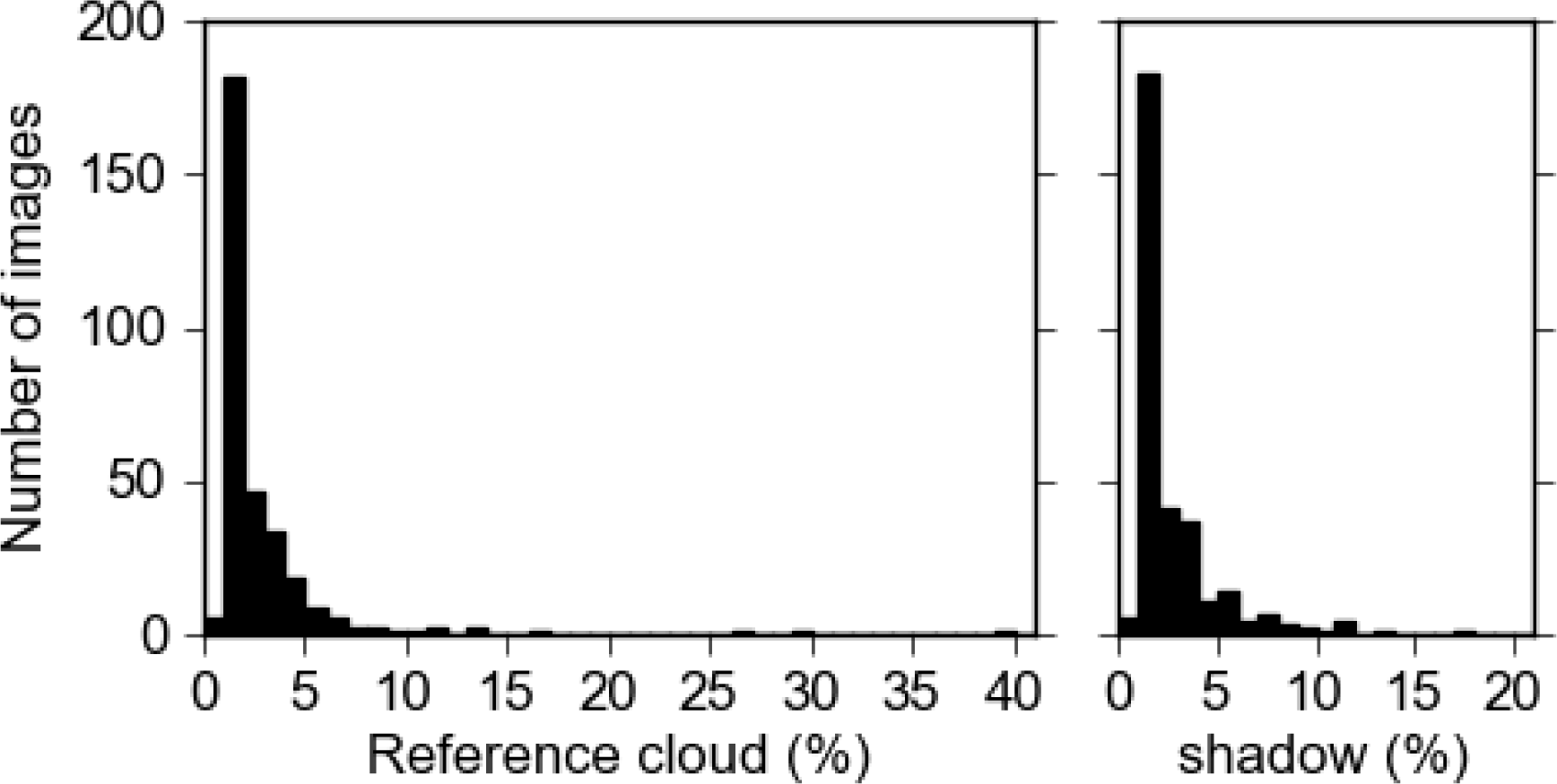
Cloud and cloud-shadow masks have been generated for each of the 313 archived images through manual editing. As OEH require a single summer image coverage for NSW they choose images with no or low cloud cover, resulting in 60% of the 313 cloudy images having less than 1% cloud and 1% shadow (Figure 4).

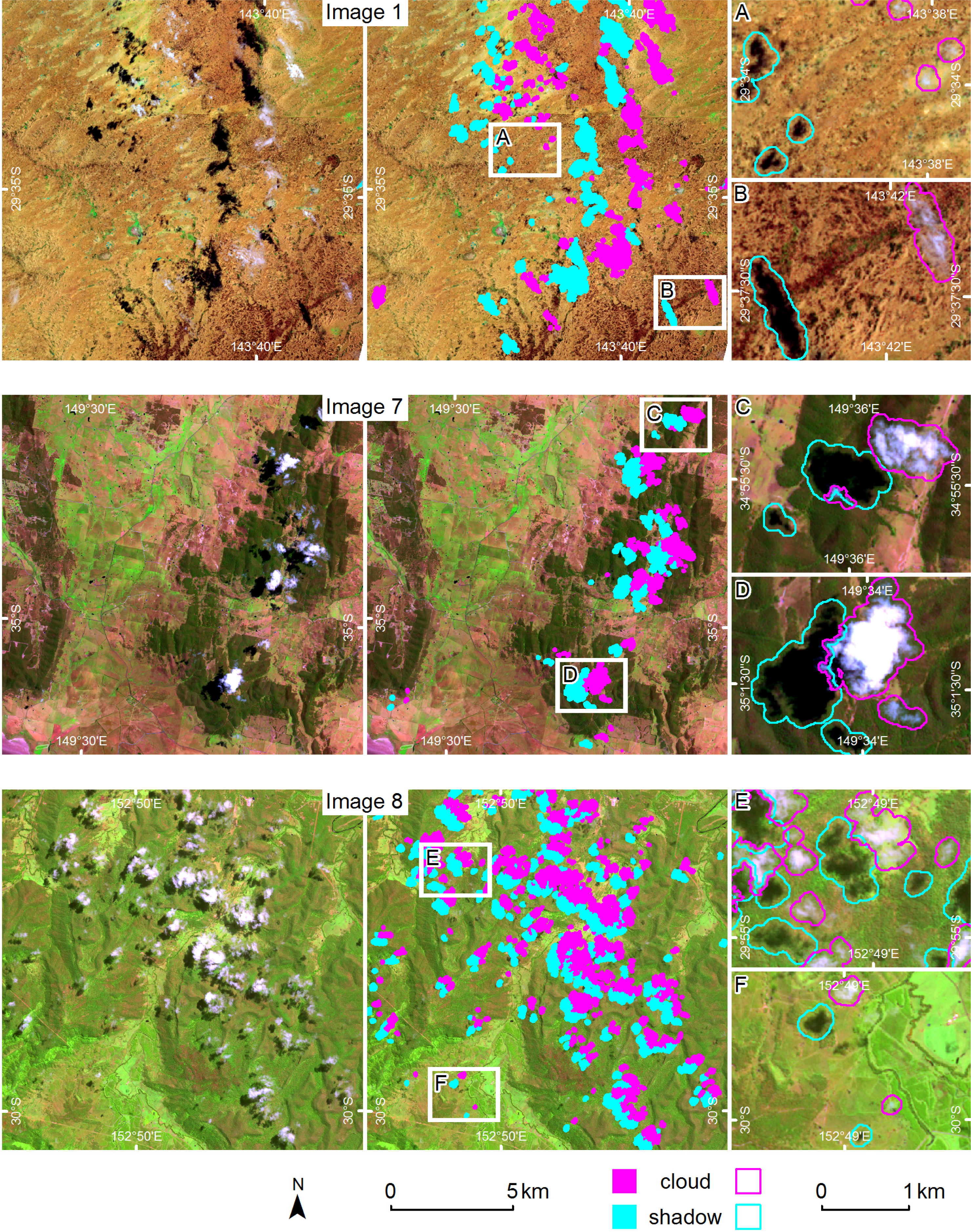
Ten of the cloudy images were selected to train SPOTCASM, due to restrictions in available time and computing resources. They were chosen to represent the variety of land cover conditions across NSW, with more images selected from the eastern part of the state, which was more often cloudy (Figure 1). They were used to test the method as it developed, through visual inspection of results at each stage. Although the manually edited masks were useful in checking the results, they could not effectively be used to optimize the methods parameters, as the manually defined edges and buffering of clouds (especially thin clouds), meant that the reference masks contained many non-cloud pixels.

3.3. Algorithm Overview

The method has several processing steps, illustrated in Figure 5, and described in the following sections. The main steps are: (1) water pixels are masked, by defining internal and external marker pixels with thresholds in green-SWIR space and growing segments; (2) vegetation pixels are masked with a threshold defined in red-NIR space; (3) possible clouds are identified by defining internal and external marker pixels with thresholds in green-SWIR space and growing segments; (4) possible shadows are identified by projecting the clouds in the required direction, searching for areas of low reflectance NIR pixels, defining internal and external markers and growing segments; and, (5) the cloud and shadow segments are refined by comparing the size of cloud and cloud-shadow pairs.

3.4. Masking Water

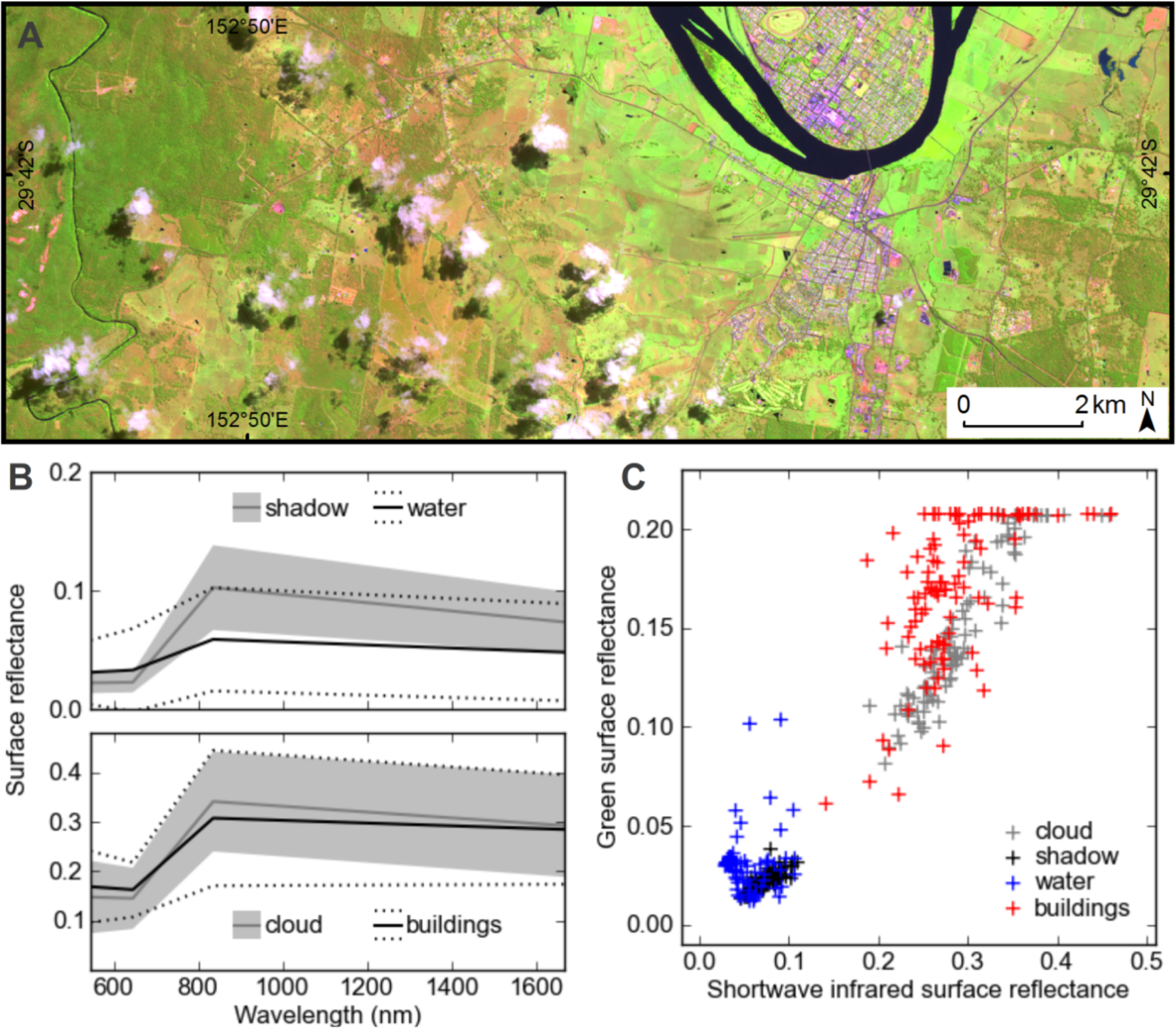
As most water pixels in SPOT5 HRG data are spectrally similar to cloud-shadows, and others are spectrally similar to clouds that are in shadow, a method to identify the majority of water pixels and remove them from further processing, without removing cloud or cloud-shadow pixels, was developed. 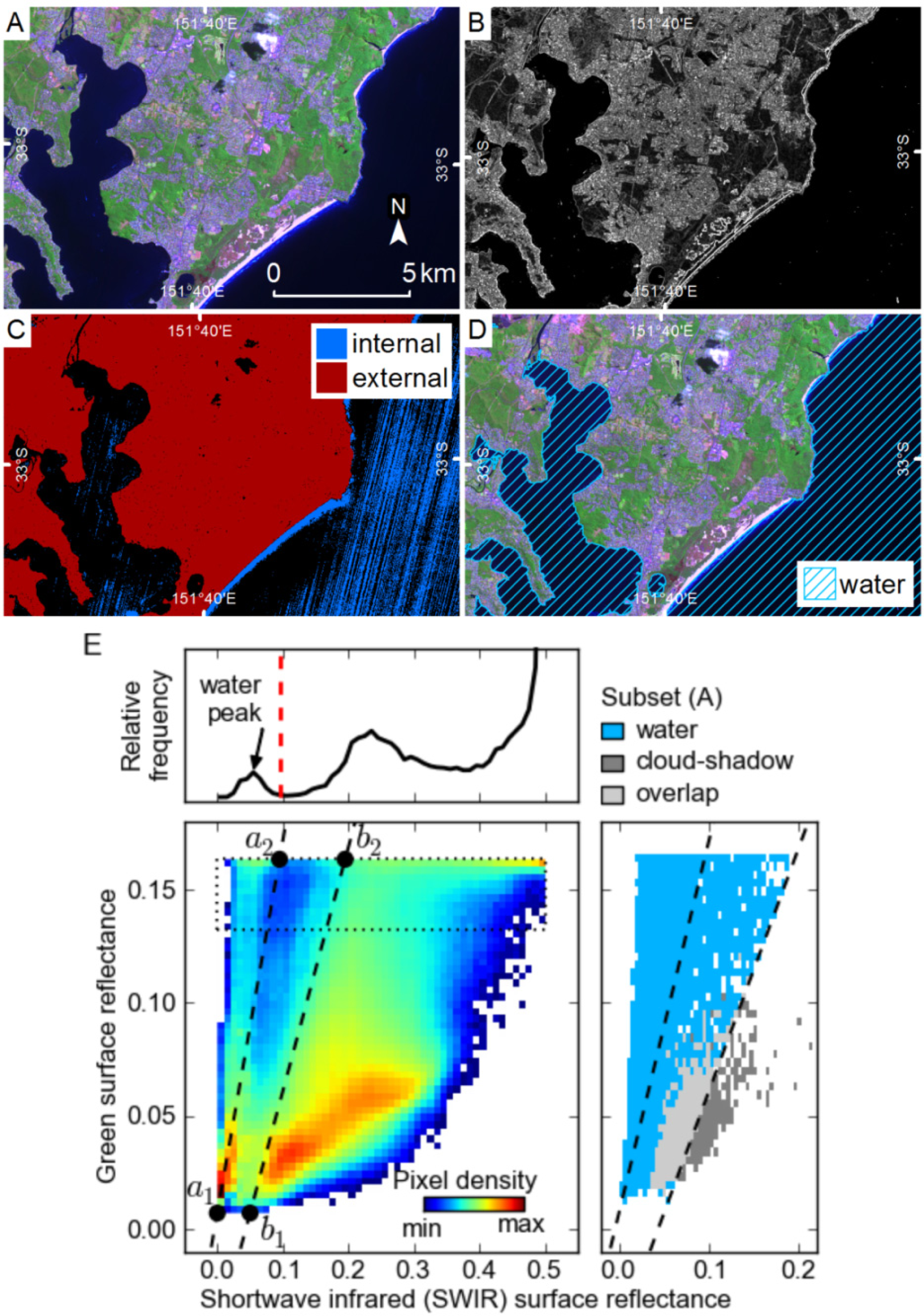Existing methods of water masking could not be used, as they have difficulty in distinguishing water from cloud-shadows [21]. Pixels in the water mask are also used as external markers when growing cloud and shadow segments with the watershed transform. For each image this method defines linear thresholds in green-SWIR space based on features in the 2-dimensional (2D) histogram constructed from those image bands. 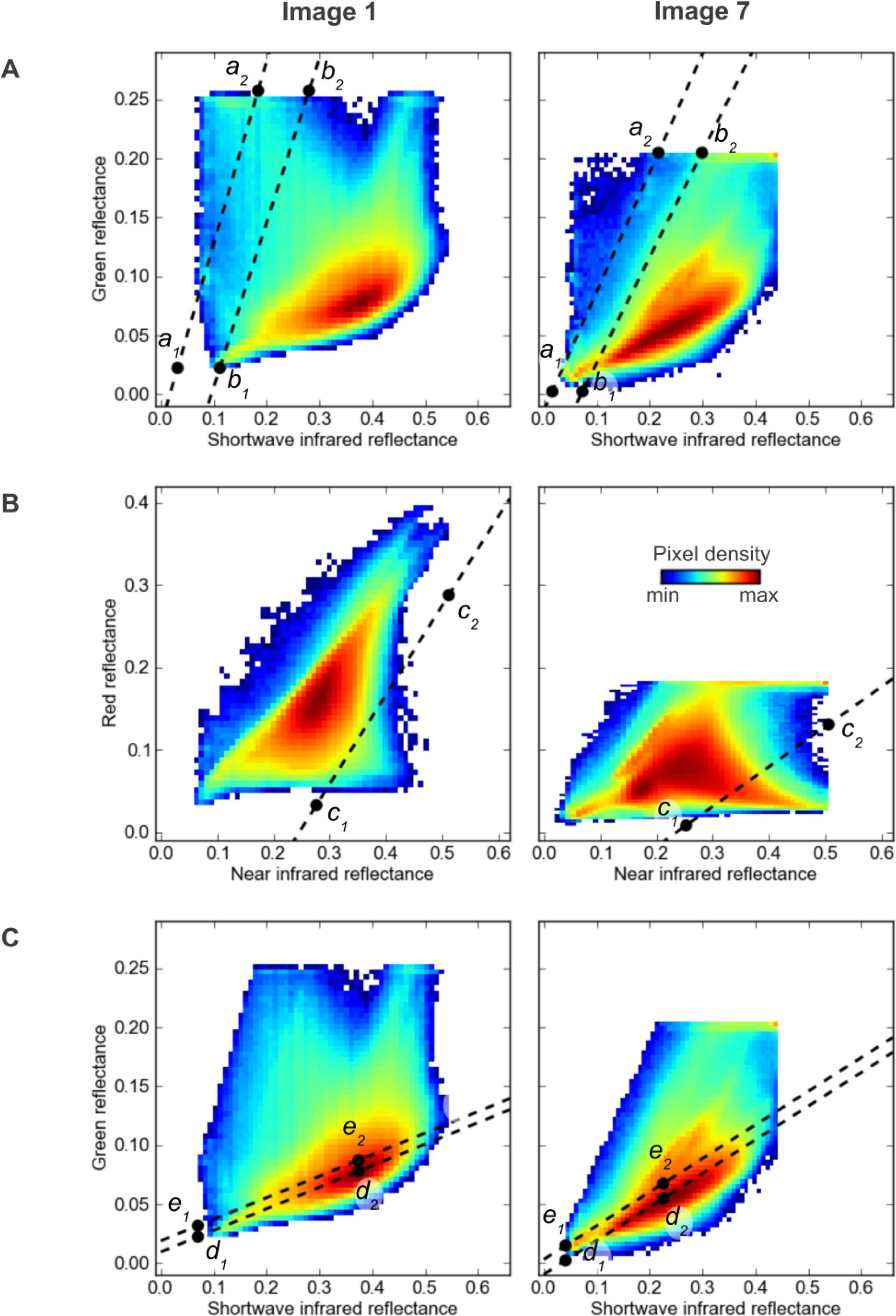An example of this method for image 9 is shown in Figure 6, and two further examples of the thresholds and 2D histograms from images 1 and 7 are shown in Figure 7A.

Firstly, a threshold is defined as line a (a₁−a₂) where pixels above a are used as internal markers for water. The second threshold is line b (b₁−b₂) where pixels below line b are external markers for water. Identifying thresholds in this way allows them to vary slightly between images that have different reflectance characteristics, examples of which are shown in Figures 6E and 7A. The points a₁, a₂, b₁ and b₂ are determined by analysis of the 2D histogram according to the following criteria: a₁ is positioned at half the minimum SWIR reflectance, and the minimum green reflectance; a₂ is defined by the location of the left edge of the rightmost peak in the top 20% of the 2D histogram, and the maximum green reflectance; b₁ and b₂ are a₁, a₂ offset in the SWIR dimension, such that b₁ is positioned at the minimum SWIR plus 10% of the maximum SWIR reflectance, and b₂ is positioned at a₂ plus 20% of the maximum SWIR reflectance. Line a is positioned to threshold all pixels with a high ratio of green to SWIR reflectance, which includes most water and snow. The position of a₁ ensures that shadow pixels with very low reflectance values are not included; while the position of a₂ ensures that clouds with lower than normal SWIR reflectance (e.g., clouds in shadow) are not included.

The markers defined by these thresholds are then used in a watershed-from-markers transform to generate a mask of water segments, based on the sum of the morphological gradient of the four bands. This approach grows segments from pixels that are definitely water, to the edge of the water features, and does not include omission errors that would result from attempting to define all water pixels with a threshold (Figure 6). The position of b₁ and b₂ is not highly critical to the end result as the morphological gradient at the edge of water bodies is usually quite prominent, and the external markers are only needed as a guide. The resulting water mask does omit some water pixels that have very low reflectance similar to shadows, but it identifies most large water bodies relatively well.

3.5. Masking Vegetation

Vegetation pixels are identified to be used as external markers when growing cloud and shadow segments with the watershed transform. These are pixels that have low red and high NIR reflectance, and they are masked by defining a threshold for each image in red-NIR space based on features in the 2D histogram constructed from those image bands (Figure 7B). This is a simple threshold defined by the line c (c₁−c₂), where pixels below c are masked as vegetation. The location of c₁ is half the range of NIR reflectance and the minimum of red reflectance; while c₂ is located at the maximum NIR reflectance and 0.7 times the range of red reflectance. The position of these points ensures that no cloud or cloud-shadow pixels are included in the mask. The approach is similar to defining a threshold on the normalized difference vegetation index (NDVI), but was preferred as some clouds were observed to have high NDVI values similar to vegetation. The segment growing approach used for the water mask was not employed for the vegetation mask as vegetation pixels are not always within discrete image objects with distinct edges. The resulting vegetation mask does not include all vegetation pixels, but it does remove the most obvious, and it provides external markers for the watershed algorithm during the growing of cloud and shadow segments.

3.6. Identifying Possible Clouds

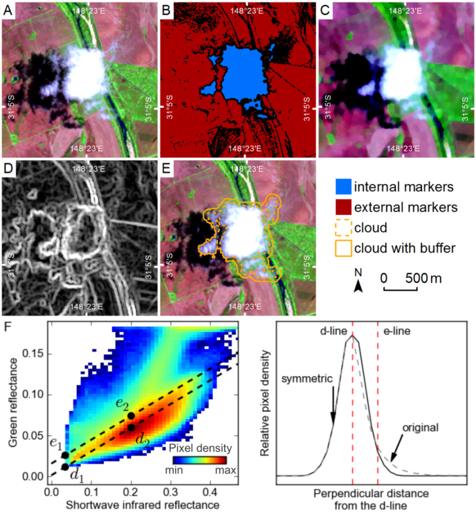
Marker pixels for clouds are defined by a threshold for each image in green-SWIR space based on features in the 2D histogram constructed from those image bands (Figures 7C and 8F), using a modified version of the method described by le Hégarat-Mascle and André [8]. The threshold is defined by the following steps. Firstly, d is identified as the line through the points d₁ and d₂, where d₁ is the minimum mid-IR and minimum green reflectance, and d₂ is the position of greatest density in the 2D histogram, after the lower 20% of values in each dimension are masked to remove the influence of shadows (Figure 8F). Line d is an approximation of the “soil line” identified by le Hégarat-Mascle and André [8]. Secondly, the 2D histogram is rotated by the slope of the line d, and the 1D signal perpendicular to the line is extracted (Figure 8F). The left-hand side of the peak in this signal (the side with greater SWIR reflectance) is not influenced by clouds, while the right-hand side of the peak contains the cloud pixels (Figure 8F). The right-hand side of the peak is discarded, and replaced by a reversed copy of the left-hand side, which makes the peak symmetric (Figure 8F). This modified histogram is then analyzed to calculate the position where 95% of the histogram is to the right. The distance from the peak to this position is used to offset points d₁ and d₂ to points e₁ and e₂ (Figure 8F). Internal marker pixels for clouds are then defined as those that have reflectance values above line e. To avoid pixels with very low reflectance being included as cloud markers, a second threshold is applied where pixels with green reflectance values less than the mean green reflectance for the whole image are removed from the cloud markers.

The threshold defined by the line e may include many other highly reflective features, such as urban structures. As many of these features are small they can be removed through morphological erosion with a 5 by 5 pixel disk-shaped structuring element. This introduces a detection limit for clouds by removing valid marker pixel objects smaller than the structuring element (50 m by 50 m).

External markers for clouds are a combination of the water and vegetation mask pixels; pixels below line d in 2D green-SWIR space, pixels with green reflectance values less than the mean green reflectance for the whole image, and pixels more than 500 m from internal marker pixels (this limits cloud growth over reflective ground that might lack external markers). Cloud segments are grown from the internal and external markers (Figure 8B) using the watershed transform on the sum of the morphological gradient for each band (Figure 8D), after an ASF has been applied (Figure 8C). The ASF removes image noise due to small objects, and enhances the edges of larger objects, while summing the morphological gradient for all bands means object edges in any band influence the segments produced by the watershed transform.

3.7. Identifying Possible Cloud-Shadows

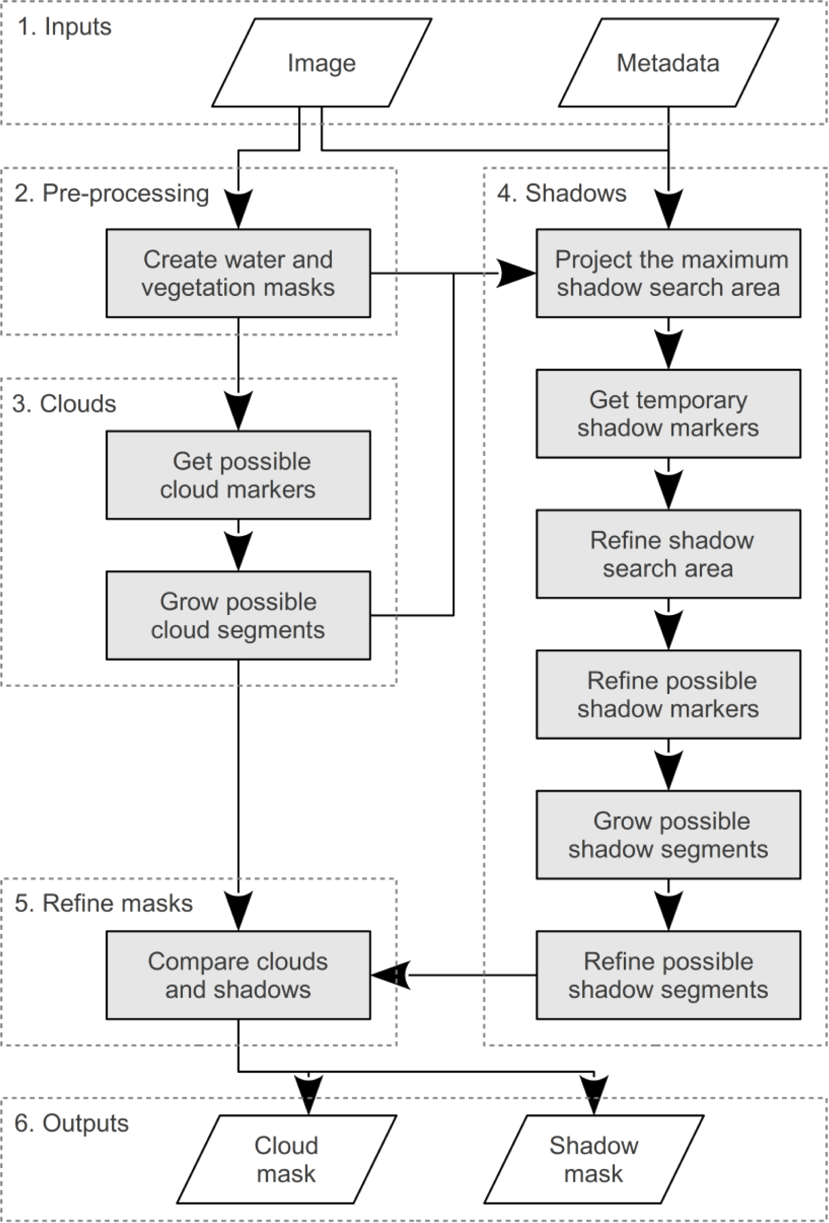
The following six steps (Figure 4) are used to identify possible cloud-shadows, each of which is described in more detail below: (1) The maximum shadow search area is calculated using the possible cloud pixels and the sun and sensor angles; (2) Temporary shadow markers are identified as all dark objects in the maximum shadow search area; (3) The maximum shadow search area is reduced by determining the optimum cloud-shadow offset distance, through comparing the possible cloud pixels and temporary shadow markers, and assuming that all clouds are at a similar height; (4) New shadow markers are defined for each of the refined shadow search areas; (5) Possible shadow segments are grown with the watershed transform using the new markers; and (6) Some of the possible shadow segments are discarded if they are too small or if they are not sufficiently darker than neighboring pixels.

The maximum cloud-shadow search area is defined by the location of the possible cloud pixels, the apparent solar azimuth and a range of possible cloud heights, in an approach similar to other methods [6,8]. Apparent solar azimuth (ϕ_a) is calculated using Equation (1).

$${\varphi }_a=\pi +\text{arctan}\left(\frac{\text{sin}{\varphi }_s\text{tan}{\theta }_s-\text{sin}{\varphi }_v\text{tan}{\theta }_v}{\text{cos}{\varphi }_s\text{tan}{\theta }_s-\text{cos}{\varphi }_v\text{tan}{\theta }_v}\right)$$

(1)

where ϕ_s is the solar azimuth, θ_s is the solar zenith, ϕ_v is the viewer (sensor) azimuth, and θ_v is the viewer zenith. Each of these inputs is taken from the image metadata file, with the approximation at the scene center used to simplify calculations. This approximation does not affect results, as other assumptions regarding flat ground and flat cloud surfaces have a greater influence on shadow location than within scene variation in sun and sensor view angles. The maximum horizontal distance between clouds and shadows is calculated using Equation (2).

$$d^2=h^2({(\text{sin}{\varphi }_s\text{tan}{\theta }_s-\text{sin}{\varphi }_v\text{tan}{\theta }_v)}^2+{(\text{cos}{\varphi }_s\text{tan}{\theta }_s-\text{cos}{\varphi }_v\text{tan}{\theta }_v)}^2)$$

(2)

where h is maximum cloud height, and d is the maximum horizontal distance between a cloud and its shadow. A maximum cloud height of 12 km was used, based on previous work [6,20], and observations of maximum cloud-shadow offsets in imagery from NSW. This may need to be increased to 18 km if processing images from the tropics [6,22]. A minimum cloud-height of zero was used, allowing for the case where cloud and shadow pixels are adjacent. The maximum shadow search area was buffered by 100 m by dilating with a disk-shaped structuring element, merging closely spaced areas into regions, and ensuring that shadow identification is not limited by the angle approximations and the assumption of flat ground and flat cloud surfaces.

Temporary shadow marker pixels are identified for each continuous region in the maximum shadow search area. They are defined using a NIR threshold, calculated by comparing the 1-dimensional histogram of NIR values from within a region with that from the surrounding pixels within a 500 m buffer. The NIR band is used as cloud shadows appeared to be consistently dark in this band compared to a variety of landcover types. As the surrounding pixels do not contain any cloud-shadows, the difference between the two histograms represents the NIR values of the shadow pixels, and an initial threshold is defined as the median value of the difference between the histograms. In regions that have generally low NIR reflectance, this initial threshold performs well in defining cloud-shadow pixels. In highly reflective regions however, the initial threshold should ideally be increased to capture more shadow pixels. These cases are identified by the presence of a distinct trough between the shadow peak and the main peak when the two histograms are added. Where this trough is identified, the initial threshold is increased to the value at the location of the trough instead of the median value of the difference.

The temporary shadow marker pixels contain any dark pixels that are in the maximum shadow search area, which can include false positives such as topographic shadow or dark patches of vegetation. By making the assumption that all clouds within an image are at approximately the same height, these errors can be reduced by using the temporary markers to calculate an optimum cloud-shadow horizontal offset, which is then used to calculate a refined shadow search area. This is implemented by iteratively shifting cloud marker pixels in the shadow direction, and for each shift calculating the percentage of cloud marker pixels that are coincident with shadow marker pixels. The position at which this percentage is at a maximum is the optimum cloud-shadow offset distance. To allow for some variation in cloud height and surface relief, this best-fit value is assigned an uncertainty of ±40 m.

New shadow markers are then determined for each possible cloud by calculating a NIR threshold for the pixels in its refined shadow search area, according to the following steps. Firstly, the percentage of pixels in the search area expected to be shadow is calculated as the number of cloud pixels divided by the number of search area pixels multiplied by 100. If the search area includes pixels off the image edge, the percentage is reduced by multiplying by the number of valid search area pixels divided by the total number of search area pixels. Secondly, a NIR threshold is calculated, such that half the expected percentage of pixels in the search area have values less than the threshold. Halving the expected percentage creates a threshold that includes only the darkest pixels as internal markers, and reduces false positives.

External markers for shadows are a combination of the pixels defined by the water and vegetation masks, and extra pixels based on local thresholds for pixels neighboring the internal markers according to the following steps. Internal markers for shadows are buffered by 500 m through dilating with a disk shaped structuring element. Local thresholds are calculated as half way between the maximum reflectance for internal marker pixels and the median reflectance for all other pixels in the buffered region, for both band 3 (NIR) and band 4 (SWIR). All pixels with reflectance values greater than these thresholds are external markers for shadows. The SWIR threshold was necessary to remove some non-shadow objects that were not sufficiently dark in the NIR alone.

Possible shadow segments are grown from the internal and external markers using the watershed transform on the sum of the morphological gradient for each band, after an ASF has been applied, following the method used for clouds. The segments are refined by size, with all segments less than 4 pixels in size removed to reduce commission of false positives from small shadows cast by tall buildings and trees, and from small water bodies that were missed by the water mask. They are further refined by only including shadows that are darker than the surrounding pixels. Shadows are deemed sufficiently dark if the mean reflectance of band 3 (NIR) for shadow pixels is at least 20% less than the mean for pixels in a 5 pixel buffer around that shadow. The value of 20% was determined by examining the reflectance of shadows and their surrounding pixels in the 10 training images. It was set to screen out obvious non-shadows without resulting in omission of real shadows.

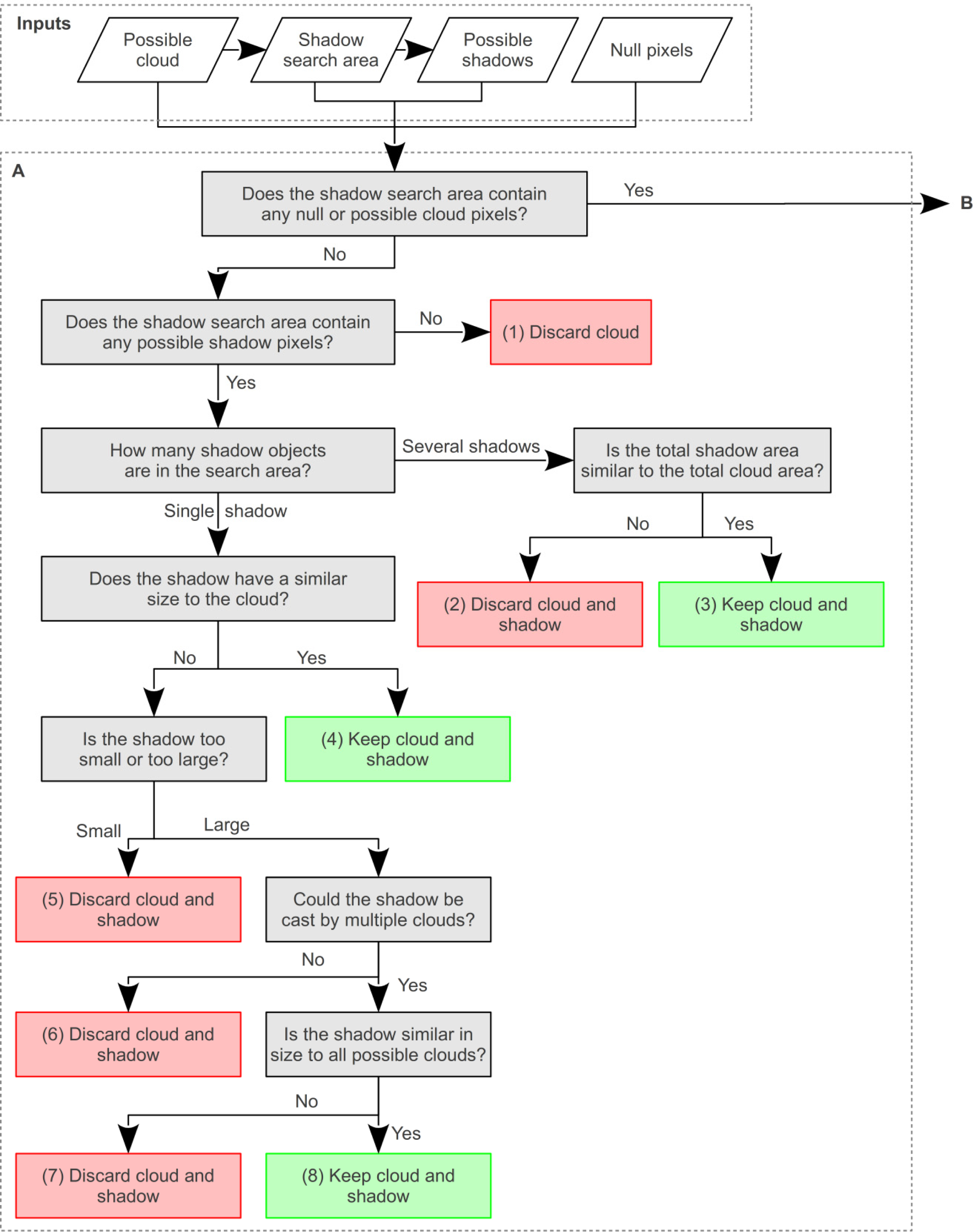
3.8. Refining Clouds and Shadows

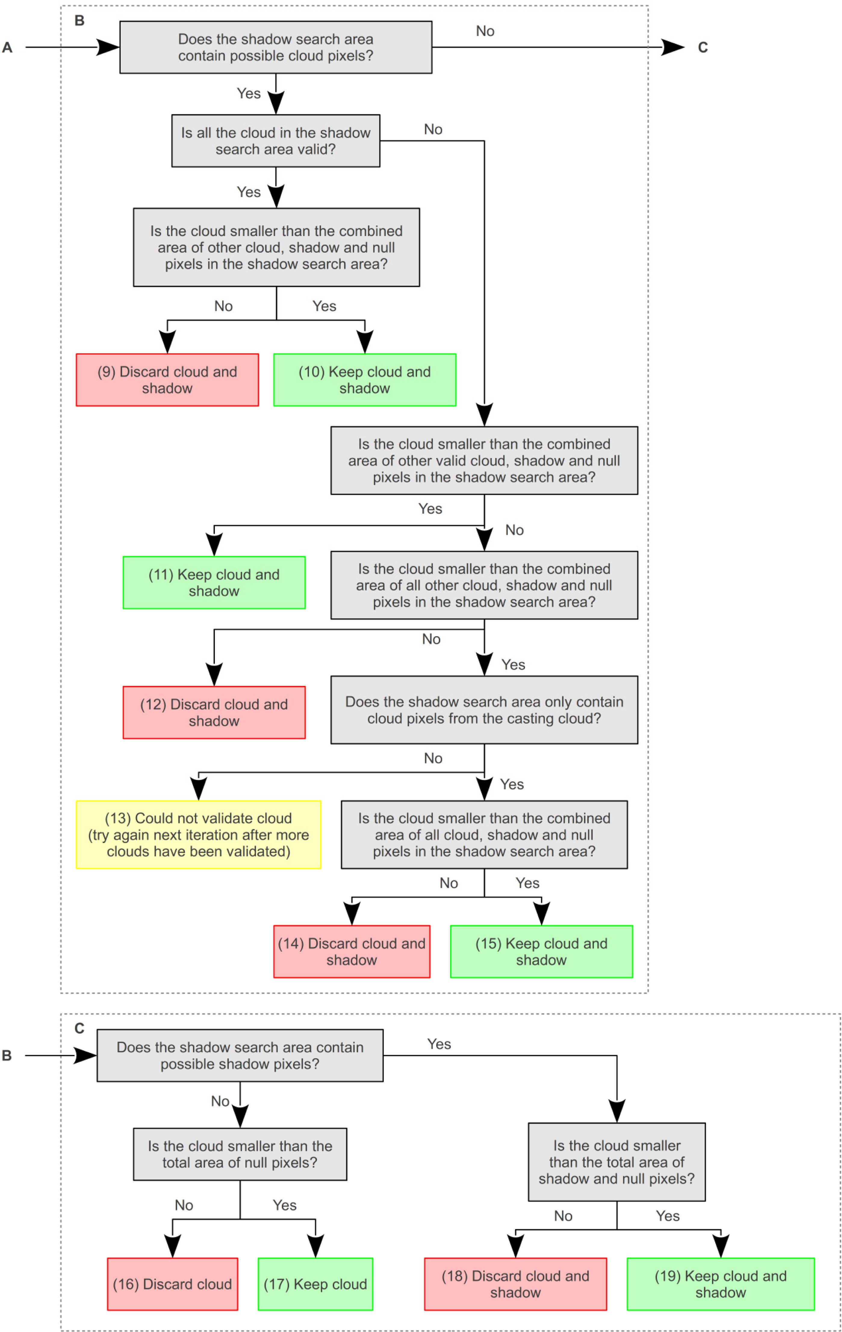
Possible cloud and shadow segments are refined through iteratively checking that each cloud object has a similar number of possible shadow pixels within the expected area, defined by the apparent solar azimuth and the best-fit cloud-shadow offset distance. This process is complicated by numerous factors, such as: the presence of possible cloud objects within the shadow search area; shadow search areas that extend off the image edge; single cloud objects that cast multiple shadow objects; and, single shadow objects that are cast by multiple cloud objects. A decision tree is used to identify whether these complicating factors are relevant to a particular cloud, before rules are applied to determine if a cloud or shadow is valid (Figure 9).

A degree of uncertainty is incorporated into any comparison of cloud and shadow size, by including a tolerance factor. When a possible cloud object has a single possible shadow object in the expected area, and no complicating factors, the cloud is considered valid if Equations (3) and (4) are true.

$$C\ge S÷t$$

(3)

$$C\le S\times t$$

(4)

where C is the size of the possible cloud (pixels), S is the size of the possible shadow (pixels) and t is the tolerance factor. After experimentation across the training images, t was set at a value of 4. This was found to be a good compromise between tolerating some variation in size (that is expected when the shadow of a 3-dimensional object is projected into a topographically varying surface) and discarding clouds and shadows that varied too greatly in size. Where Equation (3) is false, the possible cloud is deemed too large to have cast the possible shadow, and they are both discarded. Where Equation (4) is false, the possible shadow is too large for the possible cloud. If the shadow could not have been cast by additional possible clouds (checked through creating a cloud search area for the possible shadow through reversing the cloud-shadow offset distance and angle) then both possible cloud and shadow are discarded. If the possible shadow could have been cast by more than one possible cloud then the total number of cloud pixels in the cloud search area is compared to the number of shadow pixels using Equations (3) and (4) before accepting or rejecting the possible clouds and shadows.

When multiple shadows are present in the shadow search area the shadow size is calculated as the sum of all possible shadow pixels within the shadow search area, before using Equations (3) and (4). When null pixels are present in the shadow search area, these are included in the shadow size calculation, but Equation (4) is not used as the area obscured by null pixels may be much larger than the cloud size.

When other possible clouds are present in the shadow search area a different sequence of tests is used. Firstly, all the pixels from clouds that are in the shadow search area and have already been accepted are included in the calculation of shadow size. If Equation (4) is true and the cloud size is smaller than this shadow size the cloud and shadow(s) are accepted, otherwise a second step is used. This requires all cloud pixels that are in the shadow search area to be added to the shadow size even if they are yet to be validated, before testing with Equation (4). If Equation (4) is false and the cloud is larger than the shadow size, then the cloud and shadow(s) are rejected, otherwise the third step is used. This tests whether the cloud pixels within the shadow search area only belong to the cloud being validated. If this is the case, the cloud may be obscuring part of its own shadow, and both cloud and shadow(s) are accepted. If other clouds are present, then the cloud cannot be validated until the other clouds are validated first. Once all clouds have been tested, those that could not be validated are tested again, and iterations continue until all cloud has been accepted or rejected.

Other approaches to refining the clouds and shadows, such as comparing their shape [8] may perform better with discrete pairs of matching clouds and shadows. However, it is difficult to compute for all the complex situations described above and shown in Figure 9. Once the cloud and shadow masks have been finalized, they are buffered by 5 pixels through dilating with an 11 by 11 disk shaped structuring element. Any overlap created by the cloud and shadow buffering is attributed to clouds.

4. Results

SPOTCASM appears to detect the majority of thick clouds and their shadows within most of the 313 NSW images that have been validated. The application of the ASF, watershed transform and object buffering also usually ensures many thin clouds, which are often present on the edges of thick clouds, are also detected. The method works across the many landscapes of NSW, from the semi-arid shrublands in the west of the State to the agricultural and forested landscapes in the east, examples of which are shown in Figure 10. The assumption that all clouds within an image are at the same height greatly improves the masks, and was only found to be invalid in two of the 313 images.

Unfortunately, thin clouds can be completely omitted, as their spectral properties may be too similar to the ground surface. This occurred in image 2, where all of the eight clouds were thin and all were omitted (Figure 11C). Secondly, the cloud-shadow matching routine does not remove false possible clouds when there are also false possible shadows present in the expected position. This occurred in image 8, where sandy beaches and urban areas were included in the cloud mask and unmasked water bodies and darker patches of vegetation were present where shadows were expected (Figure 11E,F). Thirdly, false positive clouds whose expected shadow areas are off the image extent cannot be removed by the cloud-shadow matching routine. This occurred in image 1, where many false clouds exist close together on the left border of the image (Figure 11A,B). Although these limitations greatly affect the accuracy of the resulting masks, the errors are mostly the omission or commission of whole objects rather than poor delineation of object edges, and can often be quickly rectified through manual editing.

The accuracy of cloud and shadow classifications was assessed at the pixel level using overall accuracy, producer’s accuracy (measure of omission) and user’s accuracy (measure of commission) [9], through comparing against the manually edited reference masks from the 313 training and validation images. Overall accuracy was relatively high, with 54% of images being greater than 95%, and 95% of images having an overall accuracy greater than 85% (Figure 12).

Producer’s accuracy for cloud varied considerably from 0% in 18 images where all clouds were missed, to 100% in 3 images (Figure 12). Shadow producer’s accuracy also varied greatly, from 0%–94% (Figure 12). The large range in producer’s accuracy is caused by the variety of cloud types and amounts present across the imagery. Images containing mostly thick clouds have greater producer’s accuracy, and those with very few clouds have a greater range in producer’s accuracy.

User’s accuracy is generally lower than producer’s accuracy, and it also varies greatly for both cloud (0%–96%) and shadow (0%–100%). The large range in user’s accuracy is attributed to the great variety of land cover types present across the NSW images. For example, images with large urban areas tend to have more commission errors than images that contain mostly agricultural or forested land.

Accuracy was also assessed at the object level to reduce the influence of errors in the reference data, as the manual classification often contained non-cloud and non-shadow pixels around the edges of cloud and shadow objects. Reference cloud and shadow objects were defined using a four-connected structuring element (those pixels joined only across the diagonal were considered part of separate objects), and an object was deemed detected if it contained at least one correctly classified pixel. Object producers accuracy (the percentage of objects detected) showed similar variation to pixel producers accuracy, however, most of the variation occurs in images with less clouds and shadows (Figure 13). For example, images with less than 130 cloud objects had a mean and standard deviation cloud object producers accuracy of 56% ± 30%, while images with 130 cloud objects or more had 70% ± 18%.

5. Discussion

SPOTCASM is being routinely used in the OEH SPOT5 HRG image processing chain, producing automated cloud and cloud-shadow masks that have an overall accuracy of 85%. These masks are then manually edited to remove errors, before being used to screen out cloud and cloud-shadow contamination in landscape monitoring applications. As such monitoring often relies on multi-temporal change detection the manual removal of errors is essential, and producing automated SPOTCASM masks first greatly speeds up the time taken to produce accurate masks.

Although considerable effort was made to adapt the le Hégarat-Mascle and André [8] method into an effective automated method for detecting clouds and shadows in SPOT5 HRG imagery over NSW, the results are highly variable when compared to methods developed for other imagery [1,2]. Large omission and commission rates are common due to the variability in cloud and land cover types. The errors are attributed to the similarity of cloud and shadow pixels to features on the ground surface at the spectral and spatial resolution of the SPOT5 HRG data (Figure 2). Some omission of cloud can be attributed to cloud objects being discarded during their comparison with shadow objects. The discard rate of real cloud objects from the 313 validation images ranged from 0% to 100%, with a mean of 12%. When used operationally, the initial masks prior to the comparison with shadows are also kept, as they sometimes prove easier to edit than the final masks.

Some errors were caused by the choice of parameters used in the method (e.g., the offset distance of the line e from line d), and attempts to optimize the methods performance by using the training images to find the best parameter values were confounded by two problems. Firstly, the theory of first selecting possible cloud and shadow pixels and then calculating which are true or false has a practical limit. For example, attempts to ensure that all true clouds were included as possible clouds often resulted in so many possible cloud objects that there was no way of determining if any were false, as their possible shadows were all obscured by other false clouds. Secondly, relying on accuracy statistics to determine optimal parameter values is difficult when the reference masks contain errors.

Determining the methods accuracy was also complicated by the low number of cloud pixels and objects present in most of the images. Despite these problems the method is currently being used by OEH on all cloudy SPOT5 HRG imagery to produce an interim mask, which is then manually edited to remove visible errors.

6. Conclusions

The method described in this paper is the first published automated cloud and cloud-shadow detection routine designed specifically for Satellite pour l’Observation de la Terre 5 (SPOT5) High Resolution Geometrical (HRG) imagery, which is greatly facilitating multi-temporal environmental change detection. Automating this task for SPOT5 HRG imagery is difficult, as clouds and their shadows are very similar to features on the earth’s surface in the four available bands. The method, called SPOTCASM (SPOT cloud and shadow masking), achieved an overall accuracy of 85% for 313 images over New South Wales (NSW), Australia. It firstly uses morphological image processing to identify probable cloud and shadow objects, and secondly used object matching techniques to determine which are real.

The novel aspects of the method, such as using the watershed transform and identifying image specific thresholds on 2-dimensional image histograms, show some promise for more general image classification problems. With careful selection of markers, the watershed transform could be used for more general purpose image segmentation routines. By determining thresholds as lines in 2-dimensions, based on the shape of the histogram, classifications can be customized for images with very different characteristics. For example, the positions of threshold lines for the semi-arid image 1 and the more humid agricultural image 7 are quite different (Figure 7).

As the SPOT5 HRG images used to develop and validate the method had very small proportions of clouds (60% of images had less than 1% cloud) the method may not be appropriate for images with more cloud contamination. Further testing would also be required for images with a high proportion of snow, which is a minor land cover type in NSW.

SPOTCASM is implemented using entirely open source software, allowing future enhancements to be made, and facilitating comparisons with any new alternative methods. It takes up to two hours to complete a single image, operating on an Intel Xeon 3.00 GHz processor running 64 bit GNU/Linux. It also requires up to 6 GB of RAM, as the method requires the entire image to be read into memory.

While it is unlikely that a dense time-series method such as can be used for Landsat TM/ETM+ imagery [2], will ever be feasible for SPOT5 HRG data due to the cost, it may be possible to improve the current method over NSW as the government archive now contains several years of annual data. This sporadic time-series may allow some of the false positive clouds to be removed by determining those pixels that are persistently identified as possible clouds, and should improve the user’s accuracy.

References

1. Zhu, Z.; Woodcock, C.E. Object-based cloud and cloud shadow detection in Landsat imagery. Remote Sens. Environ 2012, 118, 83–94. [Google Scholar]
2. Goodwin, N.R.; Collett, L.J.; Denham, R.J.; Flood, N.; Tindall, D. Cloud and cloud shadow screening across Queensland, Australia: An automated method using Landsat TM/ETM+ time series. Remote Sens. Environ 2013, 134, 50–65. [Google Scholar]
3. Huang, C.; Thomas, N.; Goward, S.; Masek, J.; Zhu, Z.; Townshend, J.; Vogelmann, J. Automated masking of cloud and cloud shadow for forest change analysis using Landsat images. Int. J. Remote Sens 2010, 31, 5449–5464. [Google Scholar]
4. Amato, U. Statistical cloud detection from SEVIRI multispectral images. Remote Sens. Environ 2008, 112, 750–766. [Google Scholar]
5. Ackerman, S.A.; Strabala, K.I.; Menzel, W.P.; Frey, R.A.; Moeller, C.C.; Gumley, L.E. Discriminating clear sky from clouds with MODIS. J. Geophys. Res 1998, 103, 32141–32157. [Google Scholar]
6. Luo, Y.; Trishchenko, A.; Khlopenkov, K. Developing clear-sky, cloud and cloud shadow mask for producing clear-sky composites at 250-meter spatial resolution for the seven MODIS land bands over canada and north america. Remote Sens. Environ 2008, 112, 4167–4185. [Google Scholar]
7. Latry, C.; Panem, C.; Dejean, P. Cloud Detection with SVM Technique. Proceedings of the International Geoscience and Remote Sensing Symposium (IGARSS), Barcelona, Spain, 23–28 July 2007.
8. Le Hégarat-Mascle, S.; André, C. Use of markov random fields for automatic cloud/shadow detection on high resolution optical images. ISPRS J. Photogramm. Remote Sens 2009, 64, 351–366. [Google Scholar]
9. Congalton, R.G.; Green, K. Assessing the Accuracy of Remotely Sensed Data, 2nd ed.; CRC Press: Boca Raton, FL, USA, 2009; p. 193. [Google Scholar]
10. Meyer, F.; Beucher, S. Morphological segmentation. J. Vis. Commun. Image Represent 1990, 1, 21–46. [Google Scholar]
11. Dougherty, E.R.; Lotufu, R.A. Hands-On Morphological Image Processing; SPIE Press: Washington, DC, USA, 2003. [Google Scholar]
12. Oliphant, T.E. Python for scientific computing. Comput. Sci. Eng 2007, 9, 10–20. [Google Scholar]
13. Van Rossum, G.; de Boer, J. Interactively testing remote servers using the python programming language. CWI Q 1991, 4, 283–303. [Google Scholar]
14. Oliphant, T.E. Guide to Numpy, 2006. Available online: http://www.scipy.org (accessed on 3 September 2012).
15. Jones, E.; Oliphant, T.; Peterson, P. others. Scipy: Open Source Scientific Tools for Python, 2001. Available online: http://www.scipy.org (accessed on 3 September 2012).
16. Gdal—Geospatial Data Abstraction Library. Available online: http://www.gdal.org (accessed on 18 Septmeber 2012).
17. Coelho, L.P. Pymorph: Python Morphology Toolbox, 2011. Available online: https://pypi.python.org/pypi/pymorph (accessed on 14 August 2012).
18. Coelho, L.P. Mahotas: Open source software for scriptable computer vision. J. Open Res. Softw 2013, 1, e3. [Google Scholar] [CrossRef]
19. Fisher, A. SICASM: Satellite Image Cloud and Shadow Masking, 2011. Available online: http://sicasm.sourceforge.net (accessed on 1 November 2013).
20. Flood, N.; Danaher, T.; Gill, T.; Gillingham, S. An operational scheme for deriving standardised surface reflectance from Landsat TM/ETM+ and SPOT HRG imagery for eastern Australia. Remote Sens 2013, 5, 83–109. [Google Scholar]
21. Fisher, A.; Danaher, T. A water index for SPOT5 HRG satellite imagery, New South Wales, Australia, determined by linear discriminant analysis. Remote Sens 2013, 5, 5907–5925. [Google Scholar]
22. Stubenrauch, C.J. Cloud heights from TOVS Path-B: Evaluation using LITE observations and distributions of highest cloud layers. J. Geophys. Res 2005, 110. [Google Scholar] [CrossRef]
Figure 1. Location of the cloudy Satellite pour l’Observation de la Terre 5 (SPOT5) High Resolution Geometrical (HRG) images over New South Wales, Australia (2004–2012) used to train and validate the SPOT cloud and shadow masking (SPOTCASM) method. The 10 numbered scene boundaries show the location of the training images used to develop the method.
Remotesensing 06 00776f1
Figure 2. An example of the reflectance properties of selected pixels from a subset of image 8, showing the similarity of cloud to buildings, and cloud-shadow to water. (A) Image subset displayed with bands 4, 3, and 1 and red, green and blue; (B) Each spectral curve represents the mean ± two standard deviations of 100 manually sampled pixels; (C) A 2-dimensional scatterplot of the same 100 pixels, which were taken from the image subset.
Remotesensing 06 00776f2
Figure 3. Two examples of the watershed transform applied to a 1-dimensional signal. (A) When three markers are located at the three local minima, three segments are formed with boundaries (watershed lines) on the local maxima; (B) When only two markers are selected, segment 2 floods over a peak and into the neighboring trough, until a boundary is formed with segment 1.
Remotesensing 06 00776f3
Figure 4. Histograms of the amount of cloud and shadow in the 313 SPOT5 HRG reference images used for training and validation.
Remotesensing 06 00776f4
Figure 5. The six main steps of the SPOTCASM method.
Remotesensing 06 00776f5
Figure 6. (A) An example of creating the water mask for image 9. The subset is shown with bands 4, 3, 1 as red, green and blue; (B) The sum of the morphological gradient of all bands is used to define the edges of the water bodies, shown as greyscale where white is high and black is low; (C) Internal and external marker pixels for water; (D) Water mask grown using the watershed from markers algorithm; (E) Histograms used to define marker pixels. The dotted black line on the lower 2-dimensional histogram defines the area used to create the upper histogram, while the red dashed line defines the right-hand edge of the water peak and the position of a2. This method allows most water to be masked, while cloud shadows that have very similar spectral properties to water are excluded.
Remotesensing 06 00776f6
Figure 7. Examples of thresholds identified in image 1 (Left) and image 7 (Right). Image numbers are from Figure 1 and subsets of these images are shown in the results section. (A) Threshold lines for the water mask; (B) Threshold lines for the vegetation mask; (C) Threshold lines for the cloud markers.
Remotesensing 06 00776f7
Figure 8. An example of how SPOTCASM generates cloud segments. (A) A subset of image 3 shown with bands 4, 3, 1 as red, green and blue; (B) Internal and external markers; (C) An alternating sequential filter (ASF) is applied to the image to smooth within object variation while enhancing object edges; (D) The sum of the morphological gradient of each band after the ASF was applied enhances object edges, shown as greyscale where white is high and black is low; (E) Cloud objects are grown using the watershed from markers algorithm, before a five pixel buffer is applied; (F) Thresholds for marker pixels are identified on the 2-dimensional histogram of bands 1 (green) and band 4 (SWIR). The density values along a line perpendicular to the d-line, going through point d2 are used to define the offset to the e-line.
Remotesensing 06 00776f8
Figure 9. The decision tree used to iteratively refine possible cloud and cloud-shadow objects. Any size comparison mentioned in the tree is performed using Equations (3) and (4). The numbers in the red (reject), green (accept) and yellow (no decision) rectangles identify the 19 different end-points to the decision tree. (A) The simplest case; (B) The more complicated case where possible clouds are located in the shadow search area; (C) The case complicated only by null pixels located in the shadow search area.
Remotesensing 06 00776f9aRemotesensing 06 00776f9b
Figure 10. Examples of where SPOTCASM cloud and shadow masks performed well, from subsets of images numbered in Figure 1. All images are shown with bands 4, 3, 1 as red, green and blue. Image 1 (A,B). Image 7 (C,D). Image 8 (E,F).
Remotesensing 06 00776f10
Figure 11. Examples of SPOTCASM cloud and shadow masks performed poorly, from subsets of images numbered in Figure 1. All images are shown with bands 4, 3, 1 as red, green and blue. Image 1 (A,B). Image 2 (C,D). Image 8 (E,F).
Remotesensing 06 00776f11
Figure 12. Histograms of overall accuracy, cloud producers accuracy and shadow producers accuracy for the 313 training/validation images.
Remotesensing 06 00776f12
Figure 13. The number of reference cloud and shadow objects detected in the 313 training/validation images. A reference object, defined as a 4-connected group of pixels, was classed as detected if it contained at least one classified pixel. Dashed lines represent 60%, 80% and 100% object producers accuracy.
Remotesensing 06 00776f13