Article

Airborne Measurements of CO2 Column Concentration and Range Using a Pulsed Direct-Detection IPDA Lidar

1
NASA Goddard Space Flight Center, Greenbelt, MD 20771, USA
2
Earth System Science Interdisciplinary Center, University of Maryland, College Park, MD 20740, USA
3
Sigma Space Corporation, Lanham, MD 20706, USA
4
NASA Langley Research Center, Hampton, VA 23681, USA
*
Author to whom correspondence should be addressed.
Remote Sens. 2014, 6(1), 443-469; https://doi.org/10.3390/rs6010443
Submission received: 2 October 2013 / Revised: 25 November 2013 / Accepted: 18 December 2013 / Published: 30 December 2013
(This article belongs to the Special Issue Optical Remote Sensing of the Atmosphere)

Abstract

:
We have previously demonstrated a pulsed direct detection IPDA lidar to measure range and the column concentration of atmospheric CO2. The lidar measures the atmospheric backscatter profiles and samples the shape of the 1,572.33 nm CO2 absorption line. We participated in the ASCENDS science flights on the NASA DC-8 aircraft during August 2011 and report here lidar measurements made on four flights over a variety of surface and cloud conditions near the US. These included over a stratus cloud deck over the Pacific Ocean, to a dry lake bed surrounded by mountains in Nevada, to a desert area with a coal-fired power plant, and from the Rocky Mountains to Iowa, with segments with both cumulus and cirrus clouds. Most flights were to altitudes >12 km and had 5–6 altitude steps. Analyses show the retrievals of lidar range, CO2 column absorption, and CO2 mixing ratio worked well when measuring over topography with rapidly changing height and reflectivity, through thin clouds, between cumulus clouds, and to stratus cloud tops. The retrievals shows the decrease in column CO2 due to growing vegetation when flying over Iowa cropland as well as a sudden increase in CO2 concentration near a coal-fired power plant. For regions where the CO2 concentration was relatively constant, the measured CO2 absorption lineshape (averaged for 50 s) matched the predicted shapes to better than 1% RMS error. For 10 s averaging, the scatter in the retrievals was typically 2–3 ppm and was limited by the received signal photon count. Retrievals were made using atmospheric parameters from both an atmospheric model and from in situ temperature and pressure from the aircraft. The retrievals had no free parameters and did not use empirical adjustments, and >70% of the measurements passed screening and were used in analysis. The differences between the lidar-measured retrievals and in situ measured average CO2 column concentrations were <1.4 ppm for flight measurement altitudes >6 km.

Graphical Abstract

1. Introduction

Although increasing atmospheric CO2 is widely accepted as the largest anthropogenic factor causing climate change, there is considerable uncertainty about its global budget. To be useful in reducing uncertainties about carbon sources and sinks, studies have reported that space-based atmospheric CO2 measurements need ∼0.3% precision and stability, on regional scales of from 10 degrees square [13] to 1–5 degrees square [4]. Several groups have analyzed space missions using passive spectrometers [58], and the GOSAT mission [9] is now making global CO2 measurements from space using an FTIR spectrometer and reflected sunlight. However, limitations from sun angles, atmospheric scattering, and detector dynamic range restrict its measurements to daytime cloud-free scenes in the low and mid-latitudes. An inherent error source with space-based passive spectrometers is optical scattering from aerosols and thin clouds, particularly cirrus, in the illumination or observation paths [10,11]. Even small amounts of scattering in either of these paths modifies the optical path length and thus the total CO2 absorption measured, and so it can cause large retrieval errors even for thin cirrus clouds [11]. CO2 absorption measurements made at slant angles using km-sized footprints are also susceptible to errors caused by changes in the optical path length caused by variability of the surface reflectivity within the footprint.
To overcome these limitations, the US National Research Council’s 2007 Decadal Survey recommended a new space-based CO2 measuring mission called ASCENDS [12] using the laser absorption spectroscopy approach. The mission’s goals are to quantify global spatial distribution of atmospheric CO2 with ∼1 ppm accuracy, and quantify the global spatial distribution of terrestrial and oceanic sources and sinks of CO2 with approximately monthly time resolution. The ASCENDS approach directly measures range and offers column CO2 measurements made through thin clouds and aerosols, continuous measurements over the cloud-free oceans, at low sun angles and in darkness, all of which are major advantages over passive sensors. The ASCENDS mission organizers held a workshop in 2008 to better define the science and measurement needs and plans for future work [4]. ESA has also conducted mission definition studies for a similar space mission called A-SCOPE [3,13], and their lidar sensitivity and spectroscopic analyses have been published [14,15].

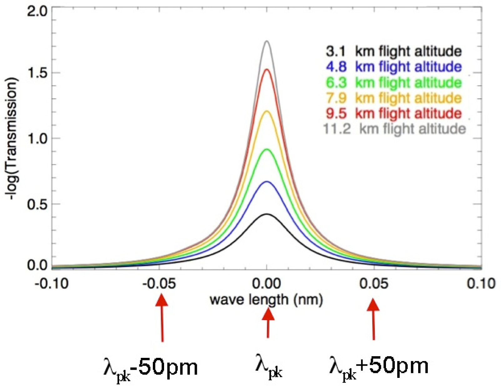
2. CO2 Line Choice and Lidar Approach

The IPDA lidar technique is widely used for open-path laser absorption spectroscopy measurements [16,17]. Typically two laser wavelengths are used, and the target is illuminated with the laser alternatively tuned onto and off the gas absorption line. The path-integrated gas absorption attenuates the on-line laser energy relative to the off-line wavelength. If one knows the difference in gas absorption cross-sections at the on- and off-line wavelengths, the elevations of the measurement endpoints, and the atmospheric temperature and pressure in the path, and measures the range and the optical depth of the gas absorption line, one can solve for the path-integrated gas number density and the column concentration. Several groups have made airborne measurements of atmospheric CO2 using IPDA lidar, and summaries have been recently published [1820].
Our airborne lidar [2124] was developed to demonstrate a dual-channel pulsed IPDA approach as a candidate for the ASCENDS mission, and a description of its configuration and its performance during flights in 2009 has been recently summarized [25]. The approach uses two tunable pulsed laser transmitters allowing simultaneous measurement of the absorption from a CO2 absorption line in the 1,570 nm band, O2 extinction in the oxygen A-band, and surface height and atmospheric backscatter in the same path. A tunable laser is stepped in wavelength across a single CO2 line for the CO2 column measurement, while simultaneously a laser is stepped across a line doublet near 765 nm in the Oxygen A-band for an atmospheric pressure measurement [2628]. Both lasers are pulsed at a 10 kHz rate, and the two absorption line regions are repeatedly sampled in wavelength steps at ∼300 Hz. Both laser transmitters utilize tunable diode lasers followed by laser amplifiers. The direct detection receivers measure the time resolved laser backscatter from the atmosphere along with the energies of the laser echoes from the surface. After suitable averaging the gas extinction and column densities for the CO2 and O2 gases are estimated from the sampled wavelengths of the surface reflected line shapes.
We use a single line in the 1,570 nm band for the CO2 measurement [10]. This vibration-rotation band of CO2 has an appropriate range of absorption that provides good sensitivity to the surface echo signal and to variation in CO2 in the lower troposphere. This band has minimal interference from other atmospheric species like H2O, and has several temperature insensitive lines. The shorter wavelength lines in the R-branch are a better match to available laser and detector technologies. The R16 line at 1,572.335 nm has been analyzed and is attractive for CO2 measurements [29]. It has low temperature sensitivity, particularly to changes in the lower atmosphere.
Our approach samples the CO2 line shape at multiple wavelengths and we used 30 samples for these flights. Sampling at multiple wavelengths across the absorption line provides several capabilities including the use of using several atmospheric weighting functions in retrievals [29]. This approach also provides information that allows solving for several different instrument parameters, such as baseline tilts, wavelength offsets, and wavelength dependent lidar transmissions. Our work has shown this information is quite important to minimize instrumental biases in retrievals. It also allows solving for useful spectroscopic information, such as line center wavelengths, line widths and errors in the fits [30].
Using pulsed lasers and receiver processing to time (and height) resolve the laser backscatter profiles also allows post detection signal processing to isolate the laser echo signals from the primary scattering surface, and to reject backscatter from the atmosphere that arrives earlier. Hence it allows isolating the full column measurement from potential bias errors caused by atmospheric scattering [10,11]. Isolating the surface echo pulse with a time gate in receiver signal processing also substantially improves the receiver’s signal-to-noise ratio (SNR) by limiting the amount of noise from the detector and the solar background. For space missions, the photon efficiency of the lidar measurement technique is quite important, and the photon efficiencies for three IPDA lidar approaches have been recently analyzed and compared [31].

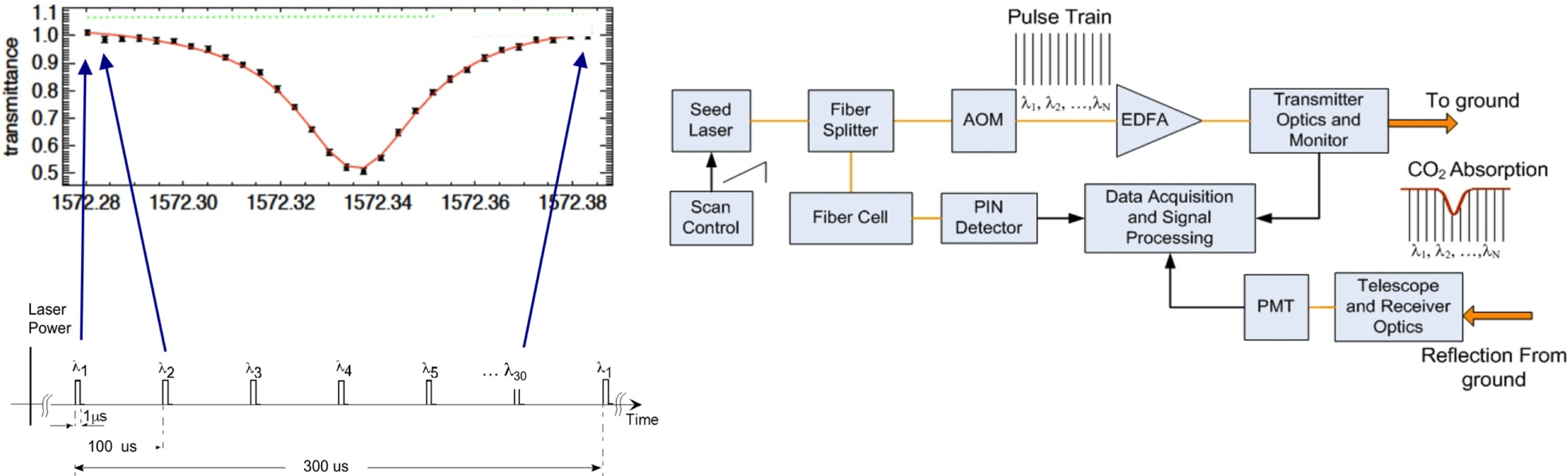
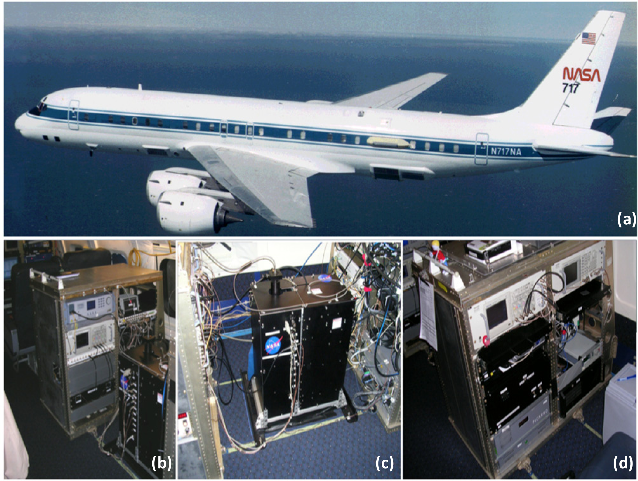
3. Airborne Lidar Description

For these flights on the NASA DC-8 aircraft [32] we adapted the previous version of the airborne lidar [25] flown on the NASA Glenn Lear-25 aircraft in 2009. A photograph of the flight configuration is shown in Figure 1. The sensor head was mounted above the aircraft’s aft-most nadir window (Port 9). The window assembly uses separate wedged and anti-reflection coated optical windows for both the transmitter and received beams to minimize optical crosstalk and etalon fringing. The airborne lidar specifications are listed in Table 1.
The approach used to sample the CO2 line and the lidar’s block diagram is shown in Figure 2. The seed source for the laser signal is a single frequency DFB laser diode, which is operated near 1,572.33 nm by controlling its temperature and current. A ramp from a signal generator was used to sweep the current to the diode laser, and hence its output wavelength. The diode’s CW output is then gated into pulses using an acousto-optic modulator (AOM) to an Erbium Doped Fiber Amplifier (EDFA). For these measurements, 30 wavelength samples are used across the CO2 line. A small percentage of the CW seed laser output is split off and directed through a fiber-coupled CO2 absorption cell and to a PIN detector. The CO2 cell serves as a monitor for center wavelength of the sweep. The laser output is a sequence of 1 us-wide laser pulses that occur at a 10 KHz rate and the collimated transmitted laser signal exits towards nadir though the transmit window.
The output laser wavelengths during the scan were precisely calibrated using a laser heterodyne technique several times during most flights in the campaign. The technique is described in Appendix A. The analysis showed that modeling the wavelength scan using 5 contiguous piecewise quadratic functions, with the slopes matched at their endpoints, would reproduce the scan wavelengths to within 0.1 pm. For the data analysis for each flight, the fits were made to calibration samples taken during that flight. If a calibration was not performed during a flight (e.g., for Iowa), data from the previous wavelength calibration was used. Analysis of the scan shape taken on different days showed little change in wavelength spacing, particularly around the CO2 absorption line peak.
The laser backscatter is collected by the receiver’s 20 cm diameter Cassegrain telescope, which views nadir through the receiver window. A multimode fiber is used to couple the optical signal from the telescope focal plane to the receiver optics. After passing through an optical bandpass filter, the signal is focused onto a PMT detector. The electrical pulse output from the PMT was amplified and passed through a threshold detector. The gain of the PMT used in the 2011 flights allowed a single photon counting efficiency of ∼4% near 1,572 nm. Typical PMT dark count rates were 500 KHz and when viewing sunlit desert surfaces the total noise count rate from the detector was a few MHz. The pulses from the receiver’s PMT detector and discriminator are binned and accumulated by the multi-channel scalar (MCS). The MCS had a time resolution of 8 ns/bin that allowed ∼5 receiver samples on both the leading and trailing edges of the laser pulses. The start time of the MCS sweep is synchronized with the trigger for the first laser pulse of the 30, and hence the start of the pulsed wavelength sweep. Each MCS sweep contains a time-resolved histogram of PMT pulse counts vs. time. This contains the complete time resolved lidar backscatter record from the laser firing to the ground for all 30 pulses. At the end of 0.9 s, each MCS bin contains the total receiver counts for the 300 laser sweeps. Although the signal strength varied with surface reflectivity and altitude, typical received signals for off-line wavelengths were ∼9000 counts for each laser pulse. The receiver histogram record is then read and stored. The laser trigger and data acquisition are synchronized to timing markers from the GPS receiver and data was stored every second. The computer also digitizes other signals, including the inertial guidance system output from the aircraft and GPS position and time. A nadir viewing video camera also records the visible image though the nadir window.

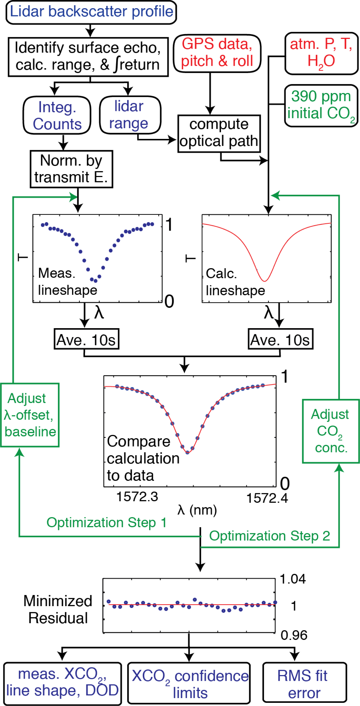
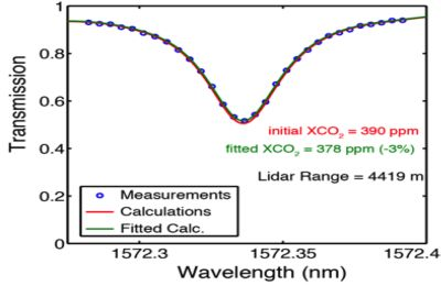
4. CO2 Measurement Processing and Retrievals

For these flights the lidar recorded the time- and wavelength-resolved laser backscatter for 300 line sweeps during each one-second recording interval. After the flight for each record we used measurement analysis approach shown in Figure 3 to process each one-second record. The range to the reflecting surface is determined using the approach described in Section 7. Figure 3 shows a typical record with an elevated cloud at a range of 5.7 km and the ground at 7.6 km. The range and pulse energies at all wavelengths can be extracted for either the strongest returns, for those nearest the predicted ground level, or for ground along with two cloud layers. Since the receiver records the entire backscatter profile at all wavelengths, this also permits extracting the wavelength-averaged range-resolved backscatter profile at the off-line wavelengths.
We followed the extraction step by the CO2 processing and retrieval algorithm shown in Figure 4. As part of the data processing step, the recorded data is tested against criteria and is screened using the algorithm described in Appendix B. For all flights, >70% of the measurements passed the screening criteria. The algorithm averages the extracted values and solves and corrects for instrumental offsets. For these flights these solved for a wavelength offset and for a slope in the lidar’s wavelength response. The algorithm then calculated the expected line shape from an atmospheric profile. This was based on either vertically resolved data from the in situ measurements during the aircraft’s spiral down maneuver (DC-8 atmosphere), or from vertically resolved data extracted from the MERRA atmospheric model at the nearest time and location to those of the measurement (MERRA atmosphere). These sources are described more fully in Section 6. The line shape calculation also accounts for the nadir angle of the aircraft, so also allows analysis of off-nadir measurements, such as those made in a banked turn.
The spectroscopic parameters for the CO2 line were from HITRAN 2008 [33] and used a line mixing correction [34]. The column average CO2 concentration in the model atmosphere is then adjusted to minimize the difference between it and the lidar observations. An example of the line fit process is shown in Figure 5, and an error analysis for the lidar measurements is summarized in [25].
Using this approach to simultaneously determine CO2 concentration and instrument model parameters considerably improves the measurement accuracy by solving and correcting for slowly varying instrument offsets and nonlinearities. After the fit several parameters are extracted including path averaged concentration, the measured line shape, the line fit’s confidence limit, and the rms error in the fit. The line fits were usually good with rms errors of <1% and typically less than twice the signal shot noise limit. From the fitted line we also compute and report the difference in the optical depths of the peak wavelength and ±50 pm offset points, that is
DOD ( pk , 50 ) = OD ( λ pk ) { OD ( λ pk 50 pm ) + OD ( λ pk + 50 pm ) } / 2
where the OD values were measured on the fitted line shapes. Examples of fitted line shapes measured at different altitudes and these points are shown in Figure 6.

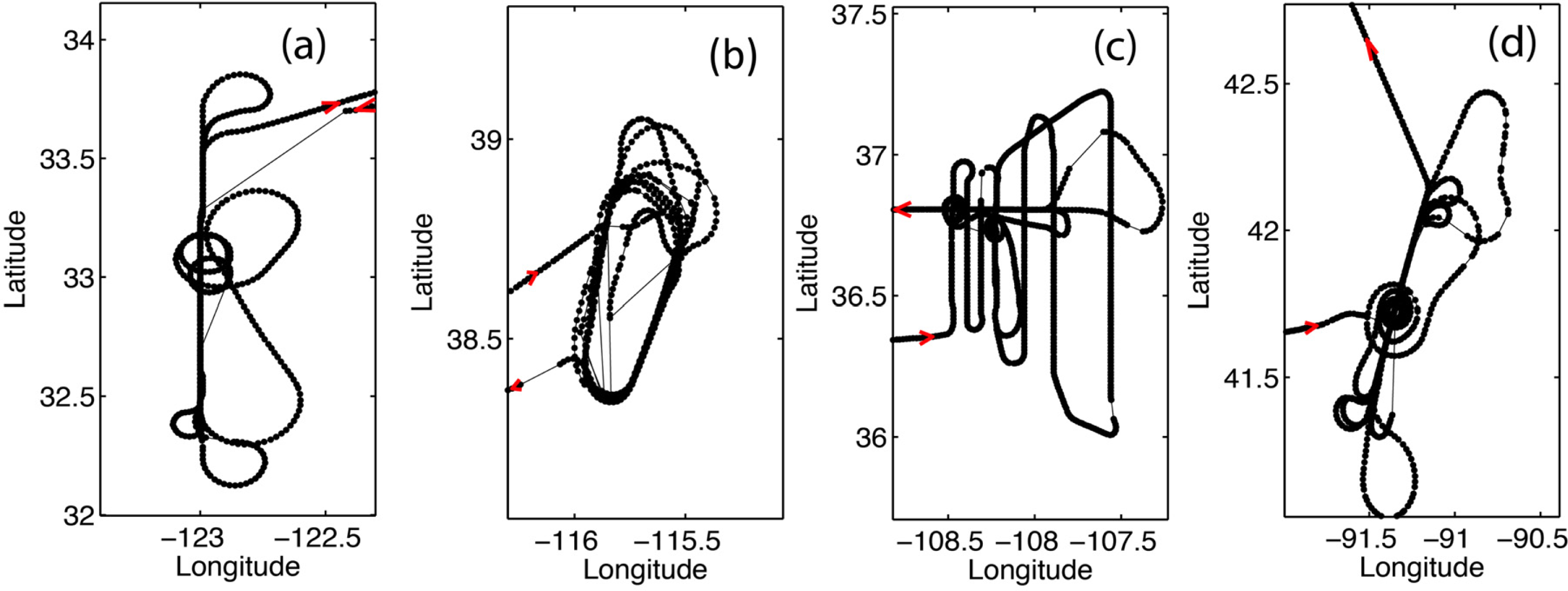
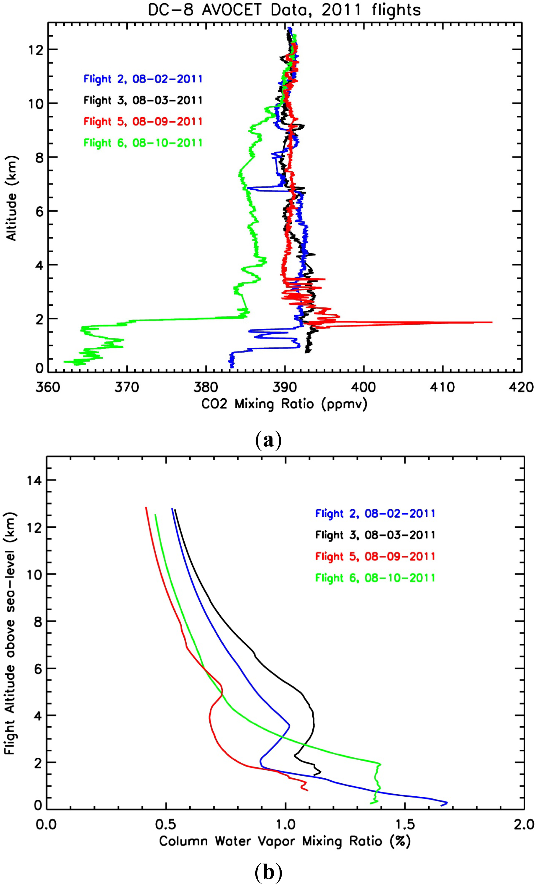
5. 2011 Airborne Campaigns

During August 2011 we flew an ASCENDS airborne campaign, and after a series of test and checkout flights, four science flights were made. Measurements were made from stepped altitudes from 3 to 13 km over locations including a stratus cloud deck over the Pacific Ocean, two desert areas in the US southwest, and over the US Midwest from the Rocky Mountains to Iowa. The flight locations, flight patterns and atmospheric conditions are summarized in Table 2 and diagrams of the flight’s ground track patterns are shown in Figure 7.
These flights allowed testing the performance of the improved lidar and optimizing the retrieval algorithms. As part of this, the lidar’s measurement of range, concentration and differential optical depth were made under a wide variety of conditions. Those were compared against predictions made using data from atmospheric model and the in situ sensors.

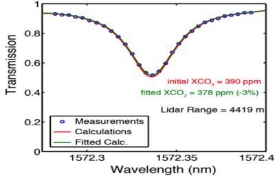
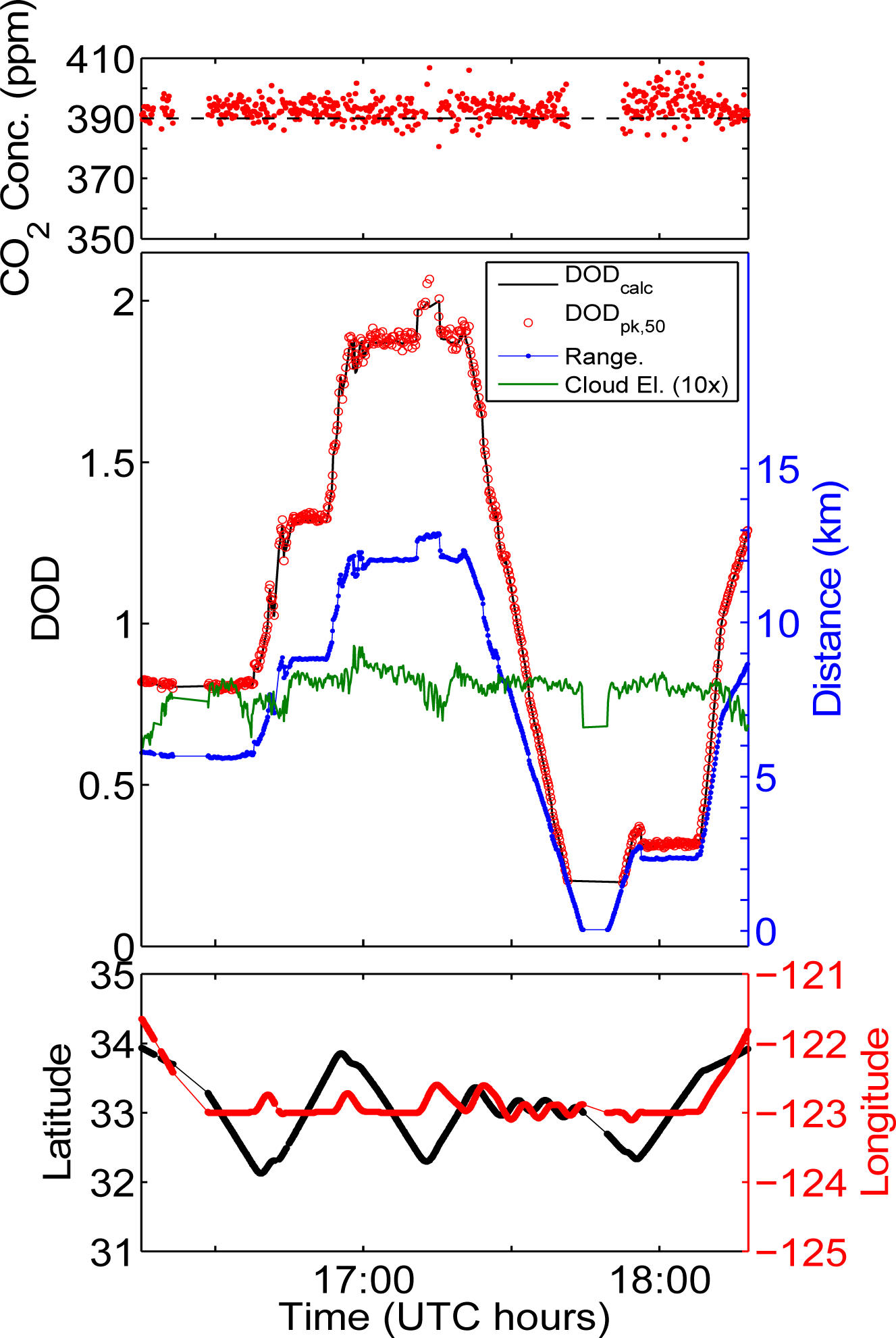
6. Airborne CO2 Measurements and Calculations

The NASA DC-8’s REVEAL instrumentation included a GPS receiver and in situ sensors for air pressure, temperature and water vapor. The LaRC AVOCET in situ CO2 sensor [35,36] was also part of the campaign and flew on the DC-8. We used readings from AVOCET gas analyzer, which reported data at a 1 Hz rate, for all comparisons of column CO2 concentrations. The altitude distribution of the CO2 concentrations measured by the AVOCET sensor is plotted in Figure 8 for the four flights. The plots show the concentrations for most flights and altitudes were near 390 ppm. There are several exceptions, including the lower concentration for Flight 6, especially below 2 km. The CO2 spike for the power plant plume for Flight 5 is also notable, as is the lower concentration below 1 km for Flight 2. The column-integrated water vapor mixing ratio is also plotted in Figure 8 for all flights. The results show that for the air columns measured in the flights the water vapor mixing ratios varied from 1% to 2% near the surface and in the boundary layers, but generally converged to 0.4% to 0.5% for columns measured from aircraft altitudes near 12 km.
In order to compute the expected line shapes and retrievals based on the lidar measurements, we used two different sources to estimate the vertical profiles of atmospheric temperature, moisture and pressure beneath the aircraft. One source was the DC-8’s REVEAL system that reported temperature, pressure and water vapor in situ readings at a 1 Hz rate. All flights had one spiral down maneuver from the highest altitude to near the surface permitting the in situ sensors to sample the entire column almost to the surface near the center of the flight pattern. Retrievals based on line shapes computed from the DC-8’s REVEAL sensor readings are the most accurate but only were available for the column at the spiral down locations.
The other approach to compute line shapes sampled values from a layered atmospheric model for the nearest location and time of day. For this we used the meteorological analysis data from the Goddard Modeling and Assimilation Office, Modern-Era Retrospective Analysis For Research and Applications (MERRA) [37]. Data were drawn from the 4/day (00, 06, 12, 18 UT) analyzed fields on the full model with 72 vertical layers on a grid of 0.5 degree latitude × 0.67 degree longitude. We extracted the latitude-longitude interpolated MERRA data at the nearest positions in time along the DC-8 flight track. The parameters extracted include surface pressure, and atmospheric pressure, geopotential height, temperature, water vapor specific humidity, and winds for the lowest 42 layers, which were sufficient to cover the DC-8 flight altitudes. Since MERRA models the atmosphere for the entire globe, this approach also allows a preview of possible retrieval results from a satellite-based lidar mission.
Figure 9 shows for the computed DOD(pk,50) vs. vertical distance above the measurement surface, with computations based on the in situ readings. To aid their comparison the plots are for the DOD(pk,50) values for the flights minus those for a US standard atmosphere with a constant mixing ratio of 390 ppm. At the same distance above the surface, the DOD values differ by several percent for the different flights. Due to the summer conditions, the air is warmer and the computed DOD(pk,50) values for the flights are lower than those of the US standard atmosphere. The colder air over the Pacific Ocean had the highest number density and computed DOD values.

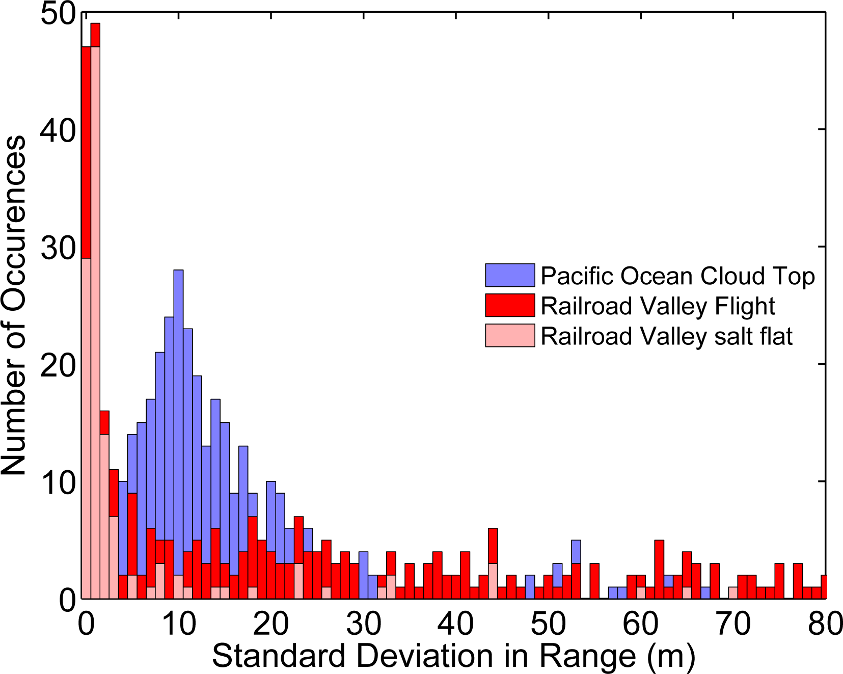
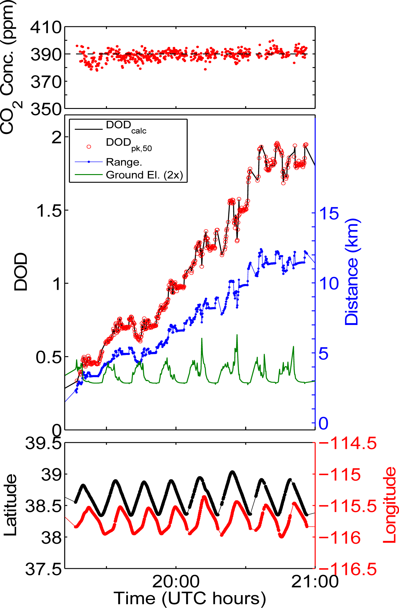
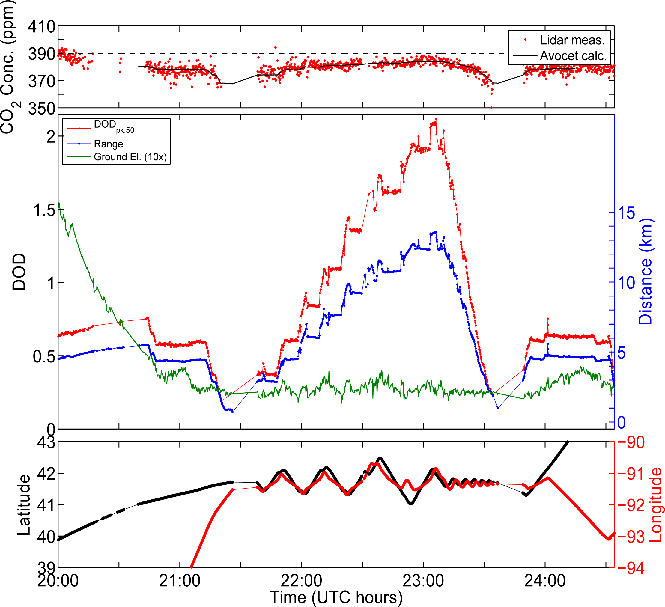
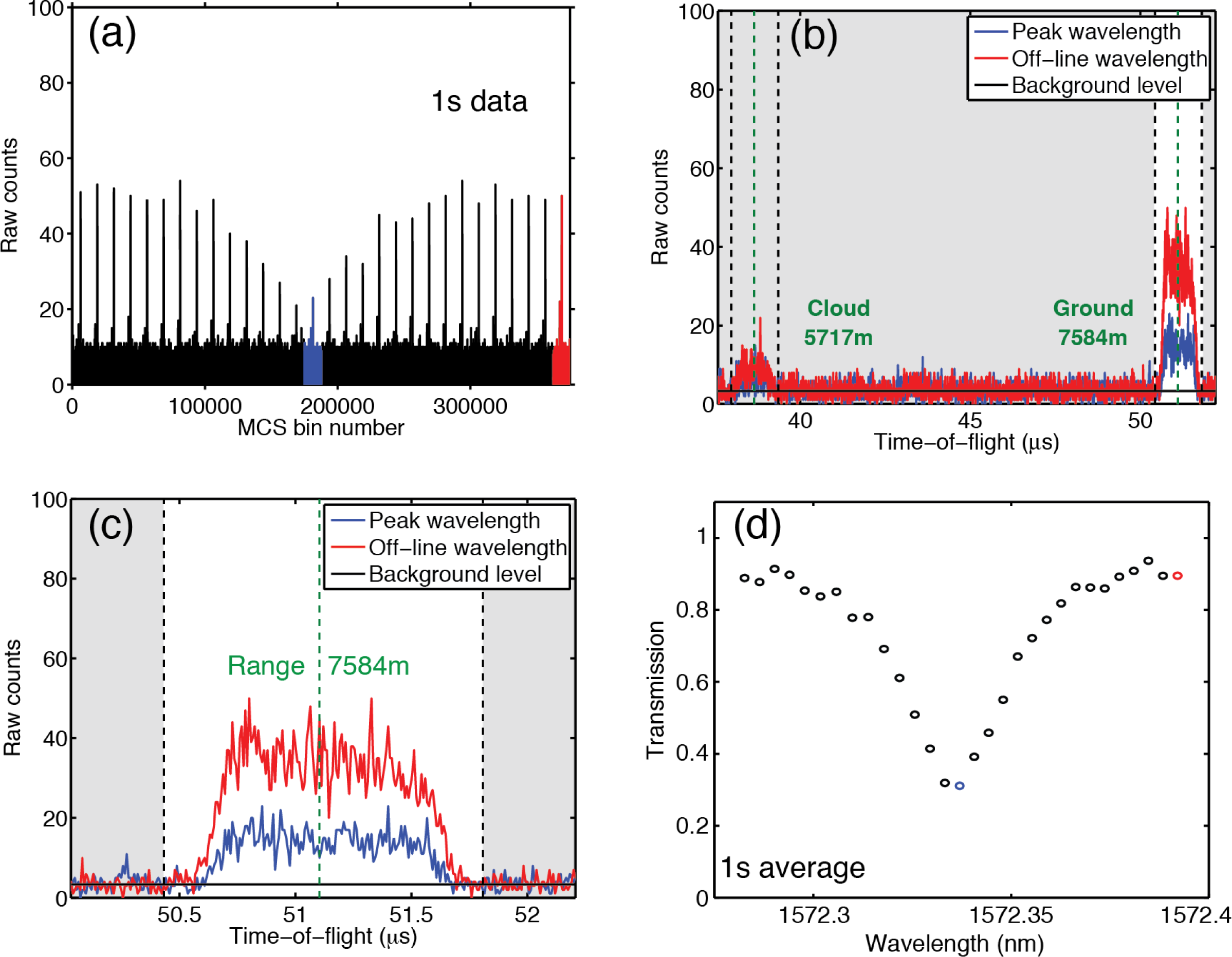
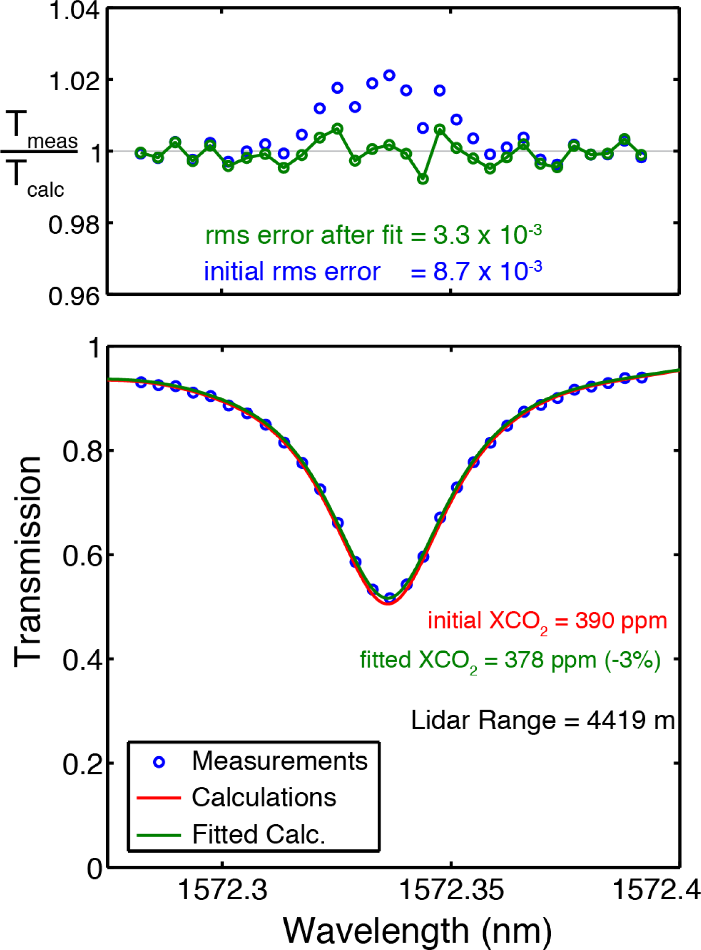
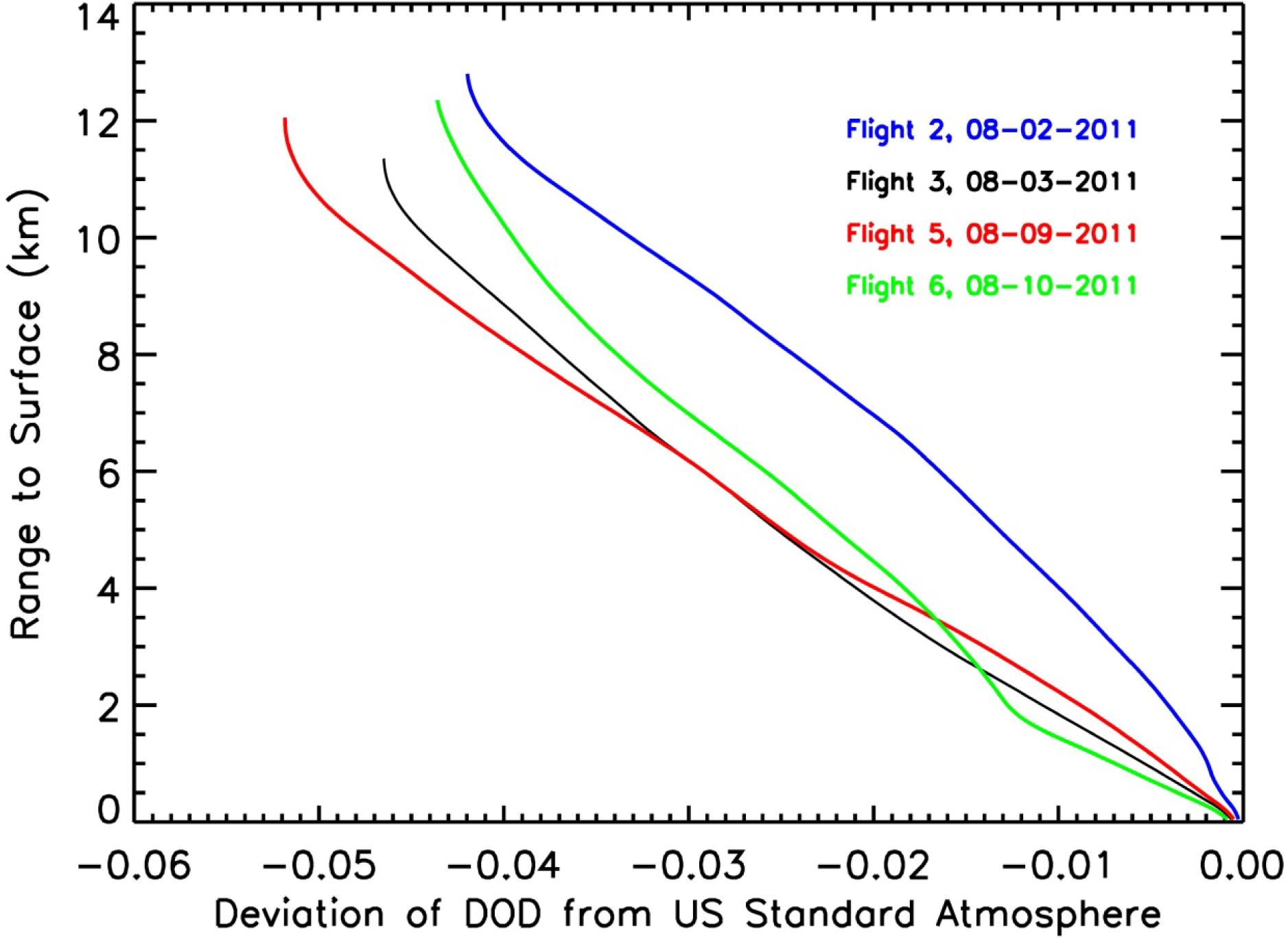
7. Range Measurements

Determining the value of the column number density and concentrations from an IPDA lidar requires an accurate measurement of range [25]. During the 1 s over which these measurements were integrated, the DC-8 aircraft travelled 200–250 m horizontally. Over flat terrain the range is usually uniform and the recorded echo pulse, averaged over 1 s, maintained the shape of the transmitted laser pulse. However, variations in the elevation of the reflecting surface over this distance (from rougher ground or cloud tops) as well as aircraft pointing and attitude changes can vary the range during the integration time. These can cause a broadening of the averaged echo pulses.
For previous work we used a cross correlation algorithm to estimate range [24]. For this analysis we used timing to the echo pulse’s centroid, which gave similar results. The precision of this ranging technique was determined from the variation in the lidar-measured range while flying level over a flat surface. We chose the flight segments over the flat playa at Railroad Valley NV and calculated at the standard deviation in the measured optical range for each 1 s of the 10 s. The median standard deviation for ∼140 of these 10 s segments was 1.2 m. The range accuracy depends on the timing accuracy of the instrument and can be biased by offsets in the receiver electronics. The lidar’s timing electronics have a timing accuracy of around 1 in 105, corresponding to a range resolution limit of <0.1 m. We measured and corrected for timing offsets to within 8 nsec or ∼1.2 m by using the reflection of the outgoing lidar pulses off the aircraft window as reference. This gives an overall accuracy of <3 m for the lidar’s optical range.
The elevation of the reflecting surfaces varied widely during these flights. Figure 10 shows a histogram of ranging precisions, made over 10 s, for measurements made to the top of the marine stratus cloud layer over the Pacific Ocean, to the mountains surrounding Railroad Valley NV, and those to the flat Railroad Valley playa. The median values of the range precisions were 12.9, 25.2 and 1.2 m respectively. The range variabilities >2 m were caused by surface elevation changes over the 10 s time (2–2.5 km distance) used for the comparison. For measurements to cloud tops, this includes any variability in the lidar pulse’s penetration into the cloud.

8. Airborne Measurement Results

Figure 11 shows the time history of the Pacific Ocean flight. During this flight the lidar measurements were made to the top of the marine stratus cloud deck from aircraft altitudes that varied from 1.5 to 13 km. The bottom panel shows measurements of range to the cloud tops, the cloud top elevation above mean sea level, the measured DOD(pk,50) values, and the predicted values for DOD(pk,50). Although some limited penetration of the lidar pulse into the cloud is expected, our present analysis does not estimate the penetration distance. The DOD measurements closely follow the range changes, due to aircraft altitude and to roll angle, and the predictions. The top panel shows the retrieved values closely track the predicted 390 ppm column average value over the entire altitude range the top panel is from column averages based on the AVOCET in situ sensor during the spiral.
Figure 12 shows a time history of measurements for the flight over Railroad Valley NV, in a similar data format. This location is a salt flat surrounded by mountains, so the oval flight had small flat segments of topography surrounded by those with rapidly varying ground elevation. Since the range is also measured by the lidar, the measured and calculated DODs follow each other closely, even as they both vary rapidly during passes over the mountains. The retrieved concentration closely follows the predicted column average value of 390 ppm calculated from the AVOCET measurements.
Figure 13 shows the time history of lidar measurements for the flight over Four Corners NM. The lidar measured values of DOD(pk,50) closely follow the range variations for the 5.5 hour flight, as expected. The retrievals also show a nearly constant CO2 concentration of ∼390 ppm over the range of flight altitudes from 3–12 km, except for a 40 ppm spike at about 17:20 UTC. This was measured when the DC-8 directly above the Four Corners coal-fired power plant.
Figure 14 shows the atmospheric conditions for the lidar measurements over Iowa. The photograph was taken from the aircraft window when over Iowa and shows an example of the cirrus and broken cumulus cloud layers that were near the spiral-down site. There are two plots of backscatter profile history on adjacent 30 min spans recorded from the lidar during the aircraft’s stair step ascent. These show the range resolved scattering from the cirrus clouds between 8–10 km altitude, from broken cumulus cloud tops at about 2 km altitude, and increased scattering from the boundary layer below 2 km. The scattering from the ground is the solid red line at a few hundred meter altitude.
Figure 15 shows the time history of the lidar measurements of range, DOD and CO2 concentrations for the Iowa flight. The range changes are from aircraft altitude changes and the increases of range during the aircraft’s banked turns are evident. The retrieved DOD values closely follow the measured range. The measurements show starting at 20 h UTC when flying eastward over the Great Plains, there is a decrease in atmospheric CO2, likely due to growing vegetation in the mid-west. The impact of the lower CO2 concentration within the boundary layer for this flight is the most noticeable in the retrievals for lower flight altitudes, where low boundary in the boundary layer is a larger column fraction, so the predicted column average is also lower. The predicted values for the column average based on the AVOCET measurements are shown in black in the top panel. Even with the presence of cirrus clouds and broken cumulus clouds the retrieved lidar values closely follow those from the in situ sensor.
Figure 16 shows a summary of the altitude resolved comparison of the column average retrievals from the lidar measurements with those measured by the AVOCET in situ sensor for all flights. The altitude resolved measurement statistics for the flights are also summarized in Table 3. In the plots the lidar measurement error bars are ±1 standard deviation for a 10 s average. Results are shown both for retrievals based on the MERRA atmospheric model and on the actual atmospheric conditions measured by the DC-8 during its the spiral maneuver. The retrievals based on the DC-8 measured atmosphere show a closer match to those from the AVOCET in situ sensor. The impact of the lower CO2 concentration in the Iowa’s flight boundary layer is evident as the trend toward smaller CO2 column densities for measurements made from lower flight altitudes. Overall the lidar retrievals are in quite good agreement with the in situ measurements, particularly for those made at 8 km and higher altitudes, and for all made over Iowa.

8. Summary

We have adapted our previously demonstrated pulsed direct detection IPDA lidar for CO2 [25] to fly on NASA’s DC-8 aircraft. The lidar measures the atmospheric backscatter profiles and shape of the 1,572.33 nm absorption line using 250 mW average laser power, 30 wavelength samples per scan with 300 scans per second. Our post-flight analysis estimates the lidar range and pulse energies at each wavelength every second. We then solve for the optimum CO2 absorption line shape, and calculated the Differential Optical Depth at the line peak and the column average CO2 concentrations. We compared these to radiative transfer calculations based on the HITRAN 2008 database, the atmospheric conditions, and the CO2 concentrations sampled by in situ sensors.
During August 2011 we participated in the ASCENDS science flights and report lidar measurements made on four flights over a variety of surface and cloud conditions near the US. These included over a stratus cloud deck over the Pacific Ocean, to a dry lake bed surrounded by mountains in Nevada, to a desert area with a coal-fired power plant, and from the Rocky Mountains to Iowa, over cloud land with both cumulus and cirrus clouds. Most flights had 5–6 altitude steps to >12 km.
Analyses show the retrievals of lidar range, CO2 column absorption, and CO2 mixing ratio worked well when measuring over topography with rapidly changing height and reflectivity, through thin clouds, between cumulus clouds, and to stratus cloud tops. The retrievals shows the decrease in column CO2 due to growing vegetation when flying over Iowa cropland as well as a sudden increase in CO2 concentration near a coal-fired power plant. For regions where the CO2 concentration was relatively constant, the measured CO2 absorption profile (averaged for 50 sec) matched the predicted profile to better than 1% RMS error. For 10 s averaging, the scatter in the retrievals was typically 2–3 ppm. The measurement precision was limited by the linear range of the PMT detector and the signal photon count for the wavelengths tuned onto the absorption line. This is consistent with the error analysis in [25]. These retrievals did not use free parameters or empirical adjustments, and >70% of the measurements passed screening and were used in analysis. The summary in Table 3 shows the differences between the mean lidar retrieved values, based on the DC-8 measured atmosphere, and the in situ measured CO2 column concentrations was <1.4 ppm for all four flights for measurement altitudes >6 km. Although the causes of these small differences are not known, we suspect a combination of instrument drift, instrument calibration errors, and small errors in the spectroscopic parameters for the CO2 line.

Acknowledgments

We are grateful for the support of the NASA Earth Science Technology Office’s Instrument Incubator Programs, the NASA ASCENDS Mission definition activity, and the NASA Goddard IRAD program. We also are grateful for the work of other members of the Goddard CO2 Sounder team, the data from the NASA LaRC’s AVOCET team, the collaborations with the NASA LaRC and JPL ASCENDS participants, and those with the DC-8 aircraft’s team members at NASA Dryden’s Airborne Operations Facility. We also appreciate the many helpful comments and suggestions from the reviewers.

Conflicts of Interest

The authors declare no conflict of interest.

References

  1. Tans, P.P; Fung, I.Y.; Takahashi, T. Observational constraints on the global atmospheric CO2 budget. Science 1990, 247, 1431–1438. [Google Scholar]
  2. Fan, S.; Gloor, M.; Mahlman, J.; Pacala, S.; Sarmiento, J.; Takahashi, T.; Tans, P. A large terrestrial carbon sink in North America implied by atmospheric and oceanic carbon dioxide data and models. Science 1998, 282, 442–446. [Google Scholar]
  3. ESA A-SCOPE Mission Assessment Report. 2008. Available online: http://esamultimedia.esa.int/docs/SP1313-1_ASCOPE.pdf (accessed on 30 August 2013).
  4. NASA ASCENDS Mission Science Definition and Planning Workshop Report. 2008. Available online: http://cce.nasa.gov/ascends/12-30-08%20ASCENDS_Workshop_Report%20clean.pdf (accessed on 30 August 2013).
  5. Kuang, Z.; Margolis, J.; Toon, G.; Crisp, D.; Yung, Y. Spaceborne measurements of atmospheric CO2 by high-resolution NIR spectrometry of reflected sunlight: An introductory study. Geophys. Res. Lett 2002, 29. [Google Scholar] [CrossRef]
  6. O’Brien, D.M.; Rayner, P.J. Global observations of carbon budget 2, CO2 concentrations from differential absorption of reflected sunlight in the 1.61 um band of CO2. J. Geophys. Res 2002, 107. [Google Scholar] [CrossRef]
  7. Dufour, E.; Breon, F.M. Spaceborne estimate of atmospheric CO2 column by use of the differential absorption method: Error analysis. Appl. Opt 2003, 42, 3595–3609. [Google Scholar]
  8. Kuze, A.; Suto, H.; Nakajima, M.; Hamazaki, T. Thermal and near infrared sensor for carbon observation Fourier-transform spectrometer on the Greenhouse Gases Observing Satellite for greenhouse gases monitoring. Appl. Opt 2009, 48, 6716–6733. [Google Scholar]
  9. Yoshida, Y.; Ota, Y.; Eguchi, N.; Kikuchi, N.; Nobuta, K.; Tran, H.; Morino, I.; Yokota, T. Retrieval algorithm for CO2 and CH4 column abundances from short-wavelength infrared spectra observations by the Greenhouse gases observing satellite. Atmos. Meas. Tech 2011, 4, 717–734. [Google Scholar]
  10. Mao, J.; Kawa, S.R. Sensitivity study for space-based measurement of atmospheric total column carbon dioxide by reflected sunlight. Appl. Opt 2004, 43, 914–927. [Google Scholar]
  11. Aben, I.; Hasekamp, O.; Hartmann, W. Uncertainties in the space-based measurements of CO2 columns due to scattering in the Earth’s atmosphere. J. Quant. Spectrosc. Radiat. Transf 2007, 104, 450–459. [Google Scholar]
  12. United States National Research Council. Earth Science and Applications from Space: National Imperatives for the Next Decade and Beyond. 2007. Available online http://www.nap.edu/ (accessed on 30 August 2013).
  13. Durand, Y.; Caron, J.; Bensi, P.; Ingmann, P.; Bézy, J.; Meynart, R. A-SCOPE: Concepts for an ESA Mission to Measure CO2 from Space with a Lidar. Proceedings of the 8th International Symposium on Tropospheric Profiling, Delft, the Netherlands, 19–23 October 2009.
  14. Ehret, G.; Kiemle, C.; Wirth, M.; Amediek, A.; Fix, A.; Houweling, S. Space-borne remote sensing of CO2, CH4, and N2O by integrated path differential absorption lidar: A sensitivity analysis. Appl. Phys 2008, 90, 593–608. [Google Scholar]
  15. Caron, J.; Durand, Y. Operating wavelengths optimization for a spaceborne lidar measuring atmospheric CO2. Appl. Opt 2009, 48, 5413–5422. [Google Scholar]
  16. Measures, R. Laser Remote Sensing: Fundamentals and Applications; Krieger Publishing: New York, NY, USA, 1992. [Google Scholar]
  17. Weitkamp, C. Lidar: Range Resolved Optical Remote Sensing of the Atmosphere; Springer: Berlin, Germany/Heidelberg, Germany/New York, NY, USA, 2005. [Google Scholar]
  18. Abshire, J.B.; Riris, H.; Allan, G.R.; Weaver, C.J.; Mao, J.; Sun, X.; Hasselbrack, W.E.; Kawa, S.R.; Biraud, S. Pulsed airborne lidar measurements of atmospheric CO2 column absorption. Tellus 2010, 62, 770–783. [Google Scholar]
  19. Spiers, G.; Menzies, R.; Jacob, J.; Christensen, L.; Phillips, M.; Choi, Y.; Browell, E. Atmospheric CO2 measurements with a 2 um airborne laser absorption spectrometer employing coherent detection. Appl. Opt 2011, 50, 2098–2111. [Google Scholar]
  20. Dobler, J.; Harrison, F.; Browell, E.; Lin, B.; McGregor, D.; Kooi, S.; Choi, Y.; Ismail, S. Atmospheric CO2 column measurements with an airborne intensity-modulated continuous wave 1.57 um fiber laser lidar. Appl. Opt 2013, 52, 2874–2892. [Google Scholar]
  21. Riris, H.; Abshire, J.; Allan, G.; Burris, J.; Chen, J.; Kawa, S.; Mao, J.; Krainak, M.; Stephen, M.; Sun, X.; et al. A laser sounder for measuring atmospheric trace gases from space. Proc. SPIE 2007, 6750. [Google Scholar] [CrossRef]
  22. Allan, G.R.; Riris, H.; Abshire, J.B.; Sun, X.; Wilson, E.; Burris, J.F.; Krainak, M.A. Laser Sounder for Active Remote Sensing Measurements of CO2 Concentrations. Proceedings of 2008 IEEE Aerospace Conference, Big Sky, MT, USA, 1–8 March 2008; pp. 1–7.
  23. Abshire, J.B.; Riris, H.; Allan, G.R.; Weaver, C.J.; Mao, J.; Sun, X.; Hasselbrack, W.E.; Yu, A.; Amediek, A.; Choi, Y.; et al. A lidar approach to measure CO2 concentrations from space for the ASCENDS Mission. Proc. SPIE 2010, 7832. [Google Scholar] [CrossRef]
  24. Amediek, A.; Sun, X.; Abshire, J.B. Analysis of range measurements from a pulsed airborne CO2 integrated path differential absorption lidar. IEEE Trans Geosci. Remote Sens 2012, 51, 2498–2504. [Google Scholar]
  25. Abshire, J.B.; Riris, H.; Weaver, C.; Mao, J.; Allan, G.; Hasselbrack, W.; Browell, E. Airborne measurements of CO2 column absorption and range using a pulsed direct-detection integrated path differential absorption lidar. Appl. Opt 2013, 52, 4446–4461. [Google Scholar]
  26. Stephen, M.; Krainak, M.; Riris, H.; Allan, G.R. Narrowband, tunable, frequency-doubled, erbium-doped fiber-amplified transmitter. Opt. Lett 2007, 32, 2073–2075. [Google Scholar]
  27. Stephen, M.A.; Mao, J.; Abshire, J.B.; Kawa, S.R.; Sun, X.; Krainak, M.A. Oxygen Spectroscopy Laser Sounding Instrument for Remote Sensing of Atmospheric Pressure. Proceedings of 2008 IEEE Aerospace Conference, Big Sky, MT, USA, 1–8 March 2008; pp. 1–6.
  28. Riris, H.; Rodriguez, M.; Allan, G.; Hasselbrack, W.; Mao, J.; Stephen, M.; Abshire, J.B. Pulsed airborne lidar measurements of atmospheric optical depth using the Oxygen A-band at 765 nm. Appl. Opt 2013, 52, 6369–6382. [Google Scholar]
  29. Mao, J.; Kawa, S.R.; Abshire, J.B.; Riris, H. Sensitivity Studies for a Space-based CO2 Laser Sounder. AGU Fall Meet. Abst. 2007. Available online: www.agu.org/meetings/fm07/(accessed on 30 August 2013). [Google Scholar]
  30. Ramanathan, A.; Mao, J.; Allan, G.R.; Riris, H.; Weaver, C.J.; Hasselbrack, W.E.; Browell, E.V.; Abshire, J.B. Spectroscopic measurements of a CO2 absorption line in an open vertical path using an airborne lidar. Appl. Phys. Lett 2013, 103, 214102. [Google Scholar]
  31. Sun, X.; Abshire, J.B. Comparison of IPDA lidar receiver sensitivity for coherent detection and for direct detection using sine-wave and pulsed modulation. Opt. Express 2012, 20, 21291–21304. [Google Scholar]
  32. NASA DC-8 Aircraft Fact Sheet. Available online: http://www.nasa.gov/centers/dryden/news/FactSheets/FS-050-DFRC.html# (accessed on 30 August 2013).
  33. Rothman, L.S.; Gordon, I.E.; Barbe, A.; ChrisBenner, D.; Bernath, P.F.; Birk, M.; Boudon, V.; Brown, L.R.; Campargue, A.; Champion, J.P.; et al. The HITRAN 2008 molecular spectroscopic database. J. Quant. Spectrosc. Radiat. Transf 2009, 110, 533–572. [Google Scholar]
  34. Lamouroux, J.; Tran, H; Laraia, A.L.; Gamache, R.R.; Rothman, L.S.; Gordon, I.E.; Hartmann, J.M. Updated database plus software for line-mixing in CO2 infrared spectra and their test using laboratory spectra in the 1.5–2.3 um region. J. Quant. Spectrosc. Radiat. Transf 2010, 111, 2321–2331. [Google Scholar]
  35. Choi, Y.; Vay, S.; Vadevu, K.; Soja, A.; Woo, J.; Nolf, S.; Sachse, G.; Diskin, G.S.; Blake, D.R.; Blake, N.J.; et al. Characteristics of the atmospheric CO2 signal as observed over the conterminous United States during INTEX-NA. J. Geophys. Res.: Atmos 2008, 113. [Google Scholar] [CrossRef]
  36. Vay, S.; Woo, J.; Anderson, B.; Thornhill, K.L.; Blake, D.R.; Westberg, D.J.; Kiley, C.M.; Avery, M.A.; Sachse, G.W.; Streets, D.G.; et al. Influence of regional-scale anthropogenic emissions on CO2 distributions over the western North Pacific. J. Geophys. Res.: Atmos 2003, 108. [Google Scholar] [CrossRef]
  37. Rienecker, M.M.; Suarez, M.J.; Gelaro, R.; Todling, R.; Bacmeister, J.; Liu, E.; Bosilovich, M.G.; Shubert, S.D.; Takacs, L.; Kim, G.-K.; et al. MERRA: NASA’s modern-era retrospective analysis for research and applications. J. Clim 2011, 24, 3624–3648. [Google Scholar]

Appendix

Appendix A: Lidar Wavelength Calibration and Monitoring

The lidar’s DFB laser seed laser is swept in wavelength by using a saw-tooth voltage ramp. The voltage from the ramp tunes the DFB seed laser ∼100 pm, and it was optimized to give constant sweep rate and a fast flyback. The power from the seed laser is divided between the transmitter and the wavelength calibration and monitoring setup using a 90/10 fiber splitter. The 10% fiber tap, used for calibration, is further divided using a 50/50 fiber splitter between a fiber coupled CO2 absorption cell and the wavelength subsystem. The ramp is repeated every 3.0 ms and the sweep and the pulse generation are carefully synchronized.
A heterodyne approach is used to monitor and calibrate the wavelength sweep of the DFB seed laser. Each calibration scan of the sweep is performed while the CO2 sounder is operating and each was completed within a few minutes. The calibration subsystem used a CW DFB laser as a optical local oscillator and reference marker, and its wavelength is monitored using an optical wavemeter with an uncertainty of ±0.2 pm (±0.3 pm at 1,500 nm). The calibration subsystem mixes the wavelength-scanning CW DFB laser seed’s output on a detector with ∼10 MHz bandwidth.
When the seed laser’s frequency is within a few megahertz of the local oscillator a heterodyne signal is generated from the detector. This beat note signal is recorded as a function of voltage ramp scan time and averaged. The statistical center of the ∼20 MHz wide burst is the seed laser’s wavelength at a particular time in the ramp The beat-note noise burst and time with respect to the start of the scan is recorded using 16 bit DAQ at a 1.25 MHz rate. The local oscillator laser is then tuned to a new wavelength and the process is repeated. By tuning the laser to 30 positions in the scan, evenly distributed in time, the wavelength of the individual pulses can be determined to ∼20 MHz in frequency. The results from the flight showed during many hours of operation, the overall wavelength span, and line spacing remains constant except for a slow drift in the wavelength at the start of the sweep. This drift of ≤50 MHz/h was also tracked in real time by using the CO2 reference cell independently of the heterodyne measurements.

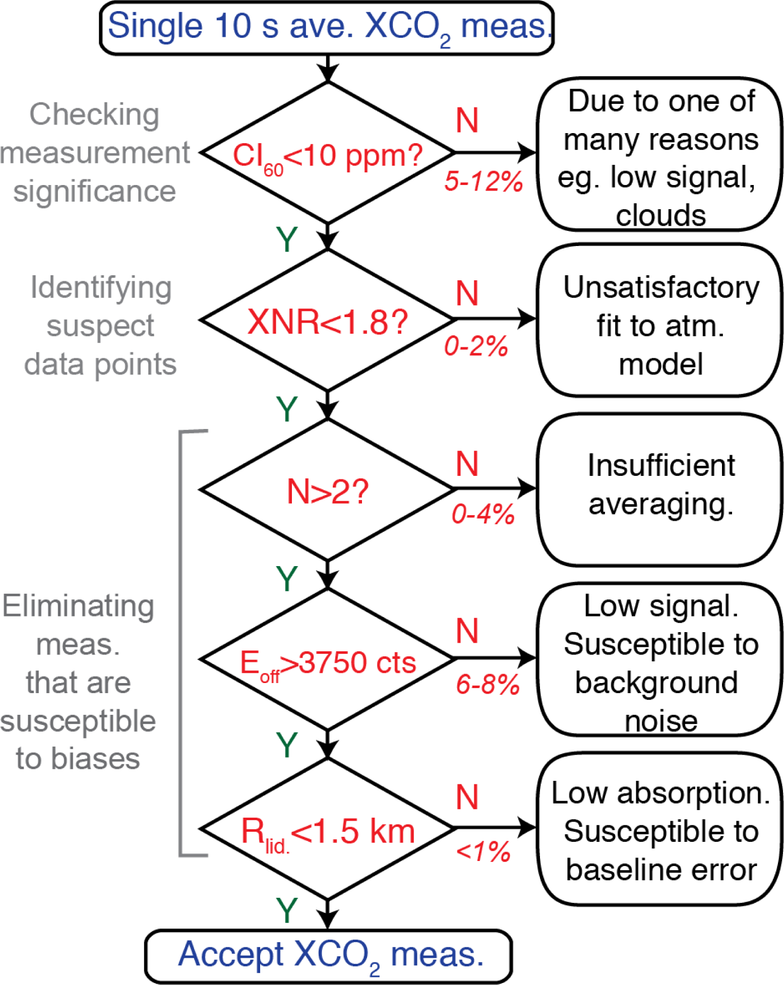
Appendix B: Lidar Data Processing and Screening

We used the automated procedure shown in Figure A1 to assess and screen the CO2 column number density measurements from the airborne lidar. The individual returns of the one-second records were first sorted by range so that cloud and surface echo pulses were separated into layers. Each layer consisted of echo pulses from the either the ground surface or a single layer of cloud top. Cloud tops were identified based on similarity in range. Once sorted by range, the echo pulse train from each layer could be averaged to reduce shot noise.
Figure A1. Screening procedure used to accept or reject the 10 s averaged lidar measurements of XCO2 for this paper. Here CI60 = 60% denotes the 60% confidence interval and XNR denotes excess noise ratio. The most common reasons for measurement rejection are given in the right side of the flowchart, and typical fractions of data rejected at each step are shown in red. The case of insufficient averaging is caused by thick clouds that block the lidar path to ground. For the regions where we made cross comparisons between lidar and Avocet measurements, >75% of 10 s data passed all the screening criteria.
Remotesensing 06 00443fa1
For the averaged data, the CO2 mixing ratio, XCO2, was then determined by adjusting it to minimize the the difference in the measured transmission lineshape T(λ) and the model lineshape, Tcalc(λ, X). That is by finding the value of XCO2 that minimized the mean square weighted sum,
χ 2 ( X ) = Σ W ( λ ) [ T ( λ ) T calc ( λ , X ) ] 2 / Σ W ( λ )
Here W(λ) is a weighting function that accounts for the relative sensitivity of T(λ) to changes in total column XCO2 and shot noise, and is given by
W ( λ ) = P ( λ ) OD ( λ ) / [ P ( λ ) + B ] .
In this expression P(λ) is the number of detected photons in the return pulse with wavelength λ, and B is the number of counts from solar background and detector dark current in each pulse.
We also calculated a confidence interval for XCO2. This gives the span of values for XCO2 within which χ2 does not increase by more than certain factor. For this analysis we chose to limit the span of χ2 to within 1.15 of χ2min corresponding to a 60% confidence interval, or
CI 60 = X ( χ 2 = 1.15 χ 2 min , X > X CO 2 ) X ( χ 2 = 1.15 χ 2 min , X < X CO 2 )
We also defined the excess noise ratio, XNR, as
XNR = [ Σ XNR ( λ ) 2 ]
where
XNR ( λ ) = [ P ( λ ) ( T ( λ ) / T calc ( λ , X CO 2 ) 1 ) 2 ]
Here P(λ) is the number of detected photons in the return pulse with wavelength λ, and T(λ) is the transmittance after adjusting the CO2 concentration.
We screened the CO2 measurements using the process shown in Figure A1. We used the size of the confidence interval, and a noise estimate as the primary screening criteria. For these flights the primary acceptance criteria were if CI60 < 10 ppm and the XNR < 1.8. The confidence interval size criterion was relaxed to 30 ppm for the cloud deck in the Pacific Ocean flight due to the weak returns from the cloud tops. The excess noise ratio limit was relaxed to 3.0 for the Railroad Valley flight owing to difficulties in modeling the mountainous terrain with MERRA.
When processing data in 10 s averaged segments, we sometimes found anomalously low measurements arising from one or more bad 1 s readings. Such bad readings often occurred when flying directly over water bodies such as the ocean, rivers, and lakes, usually due to strong specular reflections driving a nonlinear response from the detector. These usually had significant excess noise compared to the expected shot noise.
We excluded the bad readings (<10% of the 1s data), prior to averaging by processing individual 1 s data without averaging and using the initial screening criteria shown in Figure A1. Some outliers remained after screening for these criteria. These were eliminated by testing against the three additional conditions shown in Figure A1: (a) Fewer than 3 readings for averaging in a 10 s interval. Such measurements don’t average sufficiently and are susceptible to anomalies. (b) Off-line pulse counts of less than 3,750. Such readings are sensitive to small changes in the background level. (c) Lidar range < 3,750 m. Such measurements had low absorption and were sensitive to small changes in the instrument baseline. For all flights, >75% of the 10 s measurements passed all screening criteria.
Figure 1. (a) NASA DC-8 aircraft. CO2 Sounder instrument installed above Port 9 on the DC-8. (b) Rack with CO2 lidar electro-optics. (c) Enclosure with transmit optics and receiver telescope that is coupled, via fiber optics, to racks. (d) Rack with O2 lidar electro-optics in the telescope side of the rack, with flight computers on the opposite side for operators, and Picarro in situ gas analyzer.
Remotesensing 06 00443f1
Figure 2. (Left) Illustration of wavelength sampling approach, that samples the 1,572.33 nm CO2 absorption line at 30 wavelengths at a 300 Hz rate. The lidar parameters are summarized in Table 1. (Right) Block diagram of the CO2 channel of the airborne lidar.
Remotesensing 06 00443f2
Figure 3. Measurement processing approach, using examples from lidar receiver measurements with 1 s integration time from the flight over Iowa. (a) The 30 wavelength stepped laser pulses reflecting from the surface are evident in the time averaged backscatter profile, plotted with 8 ns/MCS bin. (b) A time-expanded view of a sample backscatter profile recorded for an offline pulse integrated over 1 s. This sample shows the reflected signal from a thin cloud at a distance of 5.7 km from the aircraft and the echo pulse from the ground at a range of 7.6 km. (c) Time expanded view of two pulse reflections (overlayed) from the surface, with red an offline pulse, and blue a pulse at a wavelength near the CO2 line absorption peak. (d) The photon counts for each pulse are computed by summing the counts between the pulse edges, and with the wavelength scan calibration give the transmission shape for the CO2 line. Although the atmospheric scattering above the ground causes a loss of energy, the measured shape of the CO2 line in the column to the ground is otherwise unaffected.
Remotesensing 06 00443f3
Figure 4. Data analysis and retrieval approach used to fit the CO2 lineshape and determine column average CO2 abundance and other parameters. The MCS record of the backscatter profile is analyzed to identify the pulse edges, solve for range, and determine the integrated counts as shown in Figure 3. These are then normalized by the transmit energy monitor data to give the measured lineshape. In parallel, the algorithm computes the predicted lineshape based on the optical path traveled by the lidar pulses, the atmospheric conditions of the time. The vertically resolved atmospheric state is computed using either in situ measurements from the aircraft’s spiral down manuever or data from the MERRA atmospheric model. Initially the concentration of 390 ppm was used at all altitudes. The measured and predicted line shapes were independently averaged over 10 s, the measurements and calculations were compared, and the residual was computed. The algorithm then adjusts parameters to optimize the fit. It first varied the wavelength offset and instrument baseline slope (left hand side) to adjust measurements and then it varied the CO2 column concentration (right hand side) in the prediction. The result is the retrieved CO2 column concentration that minimizes the error. The RMS error in the fit, the confidence interval of the measurement, and OD values are also retrieved and are used for screening out poor fits and bad data, as described in Appendix B.
Remotesensing 06 00443f4
Figure 5. An example line shape comparison before and after the concentration adjustment. A sample 10 s averaged transmission CO2 lineshape measured (blue dots) for the Iowa flight from 4.4 km altitude. The initial comparison is to a calculated lineshape with 390 ppm concentration that gives a noticeable fit error (blue circles in top plot). After optimizing the XCO2 in the calculations to 378 ppm, there is smaller residual (green circles in top plot) and rms error. The difference between the initial calculations (red line in bottom plot) and the optimized fit for 378 ppm (green line) is small when compared to the overall transmission lineshape.
Remotesensing 06 00443f5
Figure 6. Example of fitted CO2 line shapes, plotted as optical depths, for previous airborne lidar measurements at the altitudes indicated. The optical depths at the fitted line peak and the average of the fitted values at the sides, at peak wavelength ±50 pm, are used to compute the value of DOD(pk,50) in Equation (1) shown in subsequent plots.
Remotesensing 06 00443f6
Figure 7. Ground track patterns for the flights described in this paper. (a) Pacific Ocean west of Baja California, (b) Railroad Valley NV and surrounding mountains, (c) near Four Corners NM, and (d) near Iowa City Iowa. The flight patterns were based on surface topography, air traffic and other considerations.
Remotesensing 06 00443f7
Figure 8. (a) In situ CO2 concentration vertical profile measurements from AVOCET in the spiral-down segments of the four flights in August 2011 over the Pacific Ocean (in blue), in Railroad Valley, Nevada (in black), the Four Corners, NM (in red), and West Branch, Iowa (in green). (b) The column water vapor mixing ratios as a function of flight altitude above sea-level from the DC-8 in situ water vapor measurements for the four flights, measured during their the spiral down segment.
Remotesensing 06 00443f8
Figure 9. Plot of DOD(pk,50) calculated for the four flights from AVOCET and DC-8 in situ measurements as a function of range to surface. In order to highlight the differences, the same calculation for a US Standard Atmosphere with a vertically uniform CO2 concentration of 390 ppm was subtracted. The colder temperatures for flight 2 (over the Pacific Ocean) increased its air density and resulted in a lower difference with the US Standard atmosphere.
Remotesensing 06 00443f9
Figure 10. Examples of range precision. Histograms of the standard deviation of range measurements are plotted for measurements made, and to the tops of marine stratus clouds (blue), to mountain tops (red), and over smooth topography (pink). These were computed from 10 s groups of the 1 s measurements. For this plot, only the data was screened to exclude measurements made in turns by selecting only data collected with aircraft tilt (pitch and roll) < 30 mrad (40%–60% of data). Measurements made to the top of the marine stratus cloud deck during the Pacific Ocean flight (blue) showed a peaked histogram with a median value of 12.9 m. Measurements made over the mountains surrounding Railroad Valley NV (red) had considerable variability with a median value of 25.2 m. This spread was caused by changes in the topographic height of the mountainous terrain during the 10 s analysis interval. During the same flight the median of measurements made over the flat playa (pink) was 1.2 m, slightly higher than the lidar’s range resolution limit.
Remotesensing 06 00443f10
Figure 11. Time history of the Pacific Ocean flight over a marine layer stratus cloud deck with altitudes varying from 1.5 to 13 km. The bottom panel shows measurements of range to the cloud tops (blue), the cloud top elevation above mean sea level (green), the measured DOD values (red), and the predicted DOD values (black). The top panel shows the retrieved concentration from the lidar measurements. The measurements plotted are averaged for 10 s. The measured DOD tracks the calculated DOD throughout the flight segment. The cloud elevation is precisely determined from the lidar range and aircraft altitude, pitch and roll angles. This allows for accurate measurement of the DOD as can be seen in the upper plot. The top panel shows the retrieved values closely track the predicted 390 ppm column average value over the entire altitude range the top panel is from column averages based on the AVOCET in situ sensor during the spiral. The bottom plot shows the aircraft’s position vs. time.
Remotesensing 06 00443f11
Figure 12. Measurements for the flight over Railroad Valley NV, with the data format, colors and averaging the same as in Figure 10. This location is a flat playa surrounded by mountains, so the flight track had rapidly varying ground elevation. The measurements to the playa are evident from the flat segments in the ground elevation plot. The highly variable range and DOD are due to the varying topography, aircraft banked turns over the mountains, and the increasing aircraft altitude in successive passes over the ground track. Since the range is also measured by the lidar, the measured and calculated DODs follow each other closely, even as they both vary rapidly during passes over the mountains. The retrieved concentration closely follows the predicted column average value of 390 ppm calculated from the AVOCET measurements.
Remotesensing 06 00443f12
Figure 13. The retrieved values of range, DOD and CO2 concentrations from the lidar for the Four Corners flight, with the data format, colors and averaging the same as in Figure 10. The retrieved values of DOD from measurements closely follow the range variation during the 5.5 h long flight, as expected. They also show a nearly constant CO2 concentration of ∼390 ppm over the range of flight altitudes from 3 to 12 km, except for a 40 ppm spike at about 17:20 UTC measured directly above the Four Corners power plant. Note: The y-axis scale has been expanded to accommodate the spike. The inset shows an expanded view of flight segment from 17:10 to 17:50 UTC. This contains the spike in CO2 that causes the higher DOD value beneath the arrow.
Remotesensing 06 00443f13
Figure 14. Atmospheric conditions for measurements over Iowa. (Top) Photograph taken from the aircraft window of the cirrus and broken cumulus cloud layers over the site. (Middle) Backscatter profile history recorded from the lidar from 22:08 to 22:38 UTC. The vertical axis is elevation above mean sea level and the top of the blue band is ∼1 km below the aircraft altitude. Beneath that is the R2-corrected backscatter profile, following the color bar (linear scale) on the right. The scattering from the cirrus clouds between 8–10 km altitude, from broken cumulus cloud tops at about 2 km altitude, and the boundary layer below 2 km are evident. The ground is the solid red line at a few hundred meter altitude. (Bottom) Similar plot for the next 30 min time period of 22:39 to 23:09 UTC.
Remotesensing 06 00443f14
Figure 15. The retrieved measurements of range, DOD and CO2 concentrations for the Iowa flight, with the data format, colors and averaging the same as in Figure 10. The retrievals follow the algorithm shown in Figure 4. The retrieved DOD values closely follow the measured range. Starting at 20 h UTC when flying eastward over the Great Plains, there is a decrease in CO2 due to growing vegetation in the mid-west. The impact of the lower CO2 concentration within the boundary layer for this flight is the most noticeable in the retrievals for lower flight altitudes, where the predicted column average has a lower value. The predicted values for the column average based on the AVOCET measurements are shown in black in the top panel, and the retrieved values from the lidar follow them closely.
Remotesensing 06 00443f15
Figure 16. Comparison of column average retrievals from the airborne lidar measurements vs. altitude, for flights above the (a) Pacific Ocean, (b) Railroad Valley, (c) Four Corners NM and (d) Iowa. The plot shows lidar retrievals using the atmospheric profiles from the MERRA model (red), and those using the atmosphere sampled by the DC-8 during the spiral down (blue), and the column average CO2 values from the AVOCET in situ sensor (black). The lidar measurement error bars are ±1 standard deviation for a 10 s average, and they apply to retrievals based on MERRA and DC-8 based atmospheres. The impact of the lower CO2 concentration in the Iowa boundary layer is evident as the trend toward smaller CO2 column densities for measurements made from lower flight altitudes. The lidar retrievals based on the actual atmospheric conditions measured by the DC-8 in the spiral show a close match to those measured by the in situ sensor. Overall the lidar retrievals based on the actual atmosphere are in quite good agreement with the in situ measurements, particularly for those made at 6 km and higher altitudes. The numerical values plotted are also summarized in Table 3.
Remotesensing 06 00443f16
Table 1. 2011 Pulsed Airborne CO2 Lidar Parameters.
CO2 lineR16, 6,359.96 cm−1
CO2 line center wavelength1,572.335 nm
Laser min & max wavelengths1,572.28 nm, 1,572.390 nm
Laser wavelength steps across line30
Laser wavelength change/step∼ 3.8 pm (0.0154 cm−1)
Laser peak power, pulse width, energy25 watts, 1 μs, 25 μJ
Laser divergence angle100 μrad
Seed laser diode typeDFB: Fitel FOL15DCWD
Wavelength monitorBurleigh WA1650
Calibration heterodyne detectorNew Focus 2053-FC InGaAs
Laser Pulse Modulator (AOM)NEOS Model: 26035-2-155
Fiber coupled CO2 cell80 cm path, ∼200 Torr pressure
Fiber Laser Amplifier (EDFA)IPG EAR-10K-1571-LP-SF
Laser line scan rate300 Hz
Laser linewidth for each step∼15 MHz
Receiver Telescope typeCassegrain, f/10 (Vixen)
Telescope diameter20 cm
Receiver FOV diameter200 μrad
Receiver optical bandwidth800 pm FWHM
Receiver Optics Transmission0.64
Detector PMT typeHamamatsu H10330A-75
Detector quantum efficiency4% (these flights)
Detector dark count rate∼ 500 kHz
Receiver signal processingPhoton counting/histogramming
Histogram time bin width8 ns
Receiver integration time0.9 s per readout
Recording duty cycle90% (0.9 s every 1 s)
Table 2. Summary of 2011 Flights reported here.
Notation:Flight 2Flight 3Flight 5Flight 6
Location:Pacific OceanRailroad Valley, NVFour Corners, NMIowa
Flight Dates (all 2011)2 August3 August9 August10 August
DC-8 Spiral Down Location (Latt, Long)33°02′N38°34′N36°44′N41°43′N
122°57′W115°47′W108°13′W91°21′W
Surface Elevation (m)0*1400700235
Surface Pressure 1 (mbar)1013850924988
Approx Duration (min)264278333390
Primary Altitude range (km)3.2–12.82.9–11.24.5–12.23–12.1
Altitude step size 2 (km)31.731.5
Number of altitude steps 33–56–83–48–10
Time span of data analyzed (UTC hours)16.25, 18.319.2, 21.917.3, 20.2521.0, 23.25
Notes:
1Surface Pressure at spiral location (is listed as ocean surface for Flight 2),
*elevation of ocean surface;
2Altitude step sizes varied widely between and within flights;
3Number of altitude steps: first number indicates the number of steps after the spiral to the highest altitude. Second number indicates the total number of steps and includes any steps done before the spiral and after the highest altitude following the spiral.
Table 3. Summary of 2011 airborne measurement results. These use retrievals based on the MERRA atmospheric model as well as those on the atmosphere measured by the DC-8 aircraft in the spiral.
Location & Summary StatisticsMean Altitude (km)Min & Max Altitude (km)# of MeasOffline Single Wavel. Ave Signal (Counts)Avocet Ref. XCO2 (ppm)Lidar Mean XCO2 Based on MERRA atm (ppm)Lidar SD (ppm)Lidar Mean XCO2 Based on MERRA atm. In-situ (ppm)Lidar Mean XCO2 Based on DC-8 atm (ppm)Mean Lidar (DC-8) In-situ (ppm)
Pacific Ocean Low Cloud Top3.23.1, 4.01027,125390.9395.44.724.6389.8−1.0
Excess noise limit = 1.86.46.0, 7.01175,375391.3392.72.681.4390.0−1.3
60% conf. interval = 30 ppm7.57.0, 8.0314,625390.9392.93.272.1390.8−0.1
# process; attempts: 559/6568.58.0, 9.0415,250390.6392.12.411.6390.2−0.4
Process success rate: 85%9.59.0, 10.0684,875390.5393.52.433.0391.81.3
12.712.0, 12.81022,375390.5392.64.052.1391.71.2

RRV to Ground4.84.5, 5.0517,000392.7385.64.59−7.1389.6−3.1
Excess noise limit = 3.06.46.1, 7.01797,750391.9388.63.09−3.3391.3−0.5
60% conf. interval = 10 ppm8.08.0, 8.2417,625391.4390.02.31−1.4392.00.6
# process; attempts: 514/6329.69.0, 9.7555250391.1389.12.89−2.1390.8−0.4
Process success rate: 81%11.211.1, 11.6536,000390.9389.62.76−1.3390.8−0.1
12.812.8, 12.9846,125390.9391.42.850.5391.40.4

Four Corners to Ground4.84.0, 4.96439,500391.8384.94.63−6.9390.8−1.0
Excess noise limit = 1.86.56.4, 7.0967,625391.5387.43.62−4.1391.3−0.2
60% conf. interval = 10 ppm9.79.4, 10.0527,000391.1389.33.16−1.8391.70.6
# process; attempts: 846/971
Process success rate: 87%

Iowa to Ground3.23.0, 3.97116,000374.4375.94.601.6376.82.5
Excess noise limit = 1.84.64.0, 5.01239,000378.0377.93.290.0376.8−1.1
60% conf. interval = 10 ppm6.36.0, 7.0437,000380.0381.12.621.2381.11.1
# process; attempts: 536/7047.67.0, 8.0477,625380.8380.91.720.1381.91.1
Process success rate: 77%10.810.1, 11.0726,375382.7381.91.78−0.8383.20.4
12.512.1, 12.6815,500383.8384.12.190.3384.10.4

