Synthesis of Transportation Applications of Mobile LIDAR


Abstract
: A thorough review of available literature was conducted to inform of advancements in mobile LIDAR technology, techniques, and current and emerging applications in transportation. The literature review touches briefly on the basics of LIDAR technology followed by a more in depth description of current mobile LIDAR trends, including system components and software. An overview of existing quality control procedures used to verify the accuracy of the collected data is presented. A collection of case studies provides a clear description of the advantages of mobile LIDAR, including an increase in safety and efficiency. The final sections of the review identify current challenges the industry is facing, the guidelines that currently exist, and what else is needed to streamline the adoption of mobile LIDAR by transportation agencies. Unfortunately, many of these guidelines do not cover the specific challenges and concerns of mobile LIDAR use as many have been developed for airborne LIDAR acquisition and processing. From this review, there is a lot of discussion on “what” is being done in practice, but not a lot on “how” and “how well” it is being done. A willingness to share information going forward will be important for the successful use of mobile LIDAR.1. Introduction
This paper presents the results of an in depth review of available literature to highlight advancements in mobile light detection and ranging (LIDAR) technology, techniques, and current and emerging applications in transportation. In this synthesis, mobile LIDAR will refer solely to 3D laser scanning from a vehicular platform. It is often referred to as mobile laser scanning (MLS). Research documents were obtained from industry magazines and websites, technical reports, peer-reviewed journals, and conference presentations produced by leaders across the globe.
First, the literature review provides background on the basics of LIDAR technology followed by a more in depth description of current mobile LIDAR trends, including systems components and software. Next, this synthesis focuses on insights on current and emerging applications of mobile LIDAR for transportation agencies through industry projects and academic research. A collection of case studies provides a clear description of the advantages of mobile LIDAR, including an increase in safety and efficiency.
This review also highlights current challenges the industry is facing, the guidelines that currently exist, and what else is needed to streamline the adoption of mobile LIDAR by transportation agencies. Most existing guidelines for geospatial data are typically developed for digital terrain modeling using data from a generic source. Further, they are generally focused on elevation (vertical) error assessment, rather than 3D error assessment, which is an important consideration for many applications.
Unfortunately, many of these guidelines do not cover the specific challenges and concerns of LIDAR use. Some have been developed for airborne LIDAR acquisition and processing. However, these do not meet the needs of many transportation applications utilizing mobile LIDAR, creating a number of gaps that cannot be filled without an in depth set of guidelines developed specifically for mobile LIDAR systems. Evolving technology and limited experience with mobile LIDAR presents challenges for many organizations, which can be overcome through the development of consistent, national guidelines.
2. LIDAR Platforms
Remote assessment using LIDAR [1] can provide high speed data collection in areas with restricted access and/or safety concerns. Particularly, use of MLS on transportation corridors can minimize roadway delays. LIDAR sensors have been equipped on static ground-based platforms, and moving platforms such as airplanes, vehicles (Figure 1), boats, helicopters, UAVs, etc. In addition to powered platforms, Kukko et al. [2] have demonstrated the potential of a human carried backpack MLS system. In “Stop and Go” scanning, a static scanner is mounted to a vehicle to reduce setup time. The vehicle will periodically stop (e.g., every 100 m) and perform a scan while the vehicle is stationary. Much work has been done to develop and calibrate these devices for accurate surveying (e.g., [3–10]). The primary focus of this review pertains to mobile vehicular scanning, as opposed to airborne, railway, static terrestrial, and other platforms. Although airborne scanning has become more mainstream since the 1990s [1], increased visibility, accuracy, and resolution often require a ground-based scanning solution, particularly in transportation applications. Because static scanning has efficiency limitations, mobile scanning has become an effective solution for rapid data collection in recent years given advancements in scanning speed and accuracy, global positioning systems (GPS), and inertial measurement units (IMU). Note that static systems typically can achieve higher accuracy.
3. MLS Systems
3.1. Background and History
Prior to LIDAR based mobile mapping, other systems used a nearly identical platform setup but relied on photogrammetric methods. The first fully functional system GPSVan was created in the early 1990s by the Center for Mapping at Ohio State University. It utilized GPS, gyro, distance-measuring instrument (DMI), two CCD cameras, and a voice recorder [11].
Glennie [7] recounts the history of the first MLS system, constructed in 2003, which was initially a helicopter based LIDAR system which had been removed and mounted sideways onto a vehicle. The system was used to survey Highway 1 in Afghanistan, which was potentially hostile for helicopter based scanning. This initial system had many downfalls; primarily the limited field of view that accompanies airborne systems. However, this system proved successful and demonstrated the potential value of MLS. Currently, there are several MLS systems available through commercial vendors. Yen et al. [12] provide a comparison of many currently available mobile scan systems.
Mobile LIDAR systems provide a dense, geospatial dataset as a 3D virtual world that can be explored from a variety of viewpoints across a transportation agency. With proper practices, this dataset can serve as a 3D model to link a variety of other data such as traffic data or crash data.
3.2. Components
Puente et al. [13] compare and contrast seven commercially produced MLS systems, and though there are many MLS mapping systems, most systems consist of five distinct components:
- (1)
The mobile platform;
- (2)
Positioning hardware (e.g., GNSS, IMU);
- (3)
3D laser scanner(s);
- (4)
Photographic/video recording; and
- (5)
Computer and data storage.
3.2.1. Mobile Platform
A mobile platform connects all data collection hardware into a single system. The platform is usually a rigid platform, precisely calibrated to maintain the positional differences between the GPS, IMU, scanner(s), and imaging equipment. It also provides a means to connect to the vehicle being used in the data collection process (Figure 2).
3.2.2. Positioning Hardware
Positioning hardware varies significantly from system to system. However, at a minimum most systems incorporate at least one GPS/GNSS receiver and an IMU. The GPS/IMU systems work together to continually report the best possible position. In times of poor satellite coverage, the IMU manages the bulk of the positioning workload. However, when satellite coverage is ideal, the IMU’s positional information is then updated from the GPS [3,14]. In addition to augmenting the GPS in periods of poor satellite coverage, the IMU must continually fill gaps between subsequent GPS observations. Typical GPS receivers report positioning information at the rate of 1–10 Hz (i.e., one to 10 measurements per second). However, during the course of a second, a vehicle will experience substantial movement, particularly when traveling at high speeds. The IMU records positional information at a much higher rate, typically around 100–2,000 Hz, or 100–2,000 times per second [15,16]. GPS/IMU data quality is typically the primary factor in gaining the best accuracy for a LIDAR point cloud [17]. Barber et al. [3] explain how detailed route planning and satellite almanac checks can greatly improve accuracy with better satellite availability and geometry.
More complex MLS systems will utilize multiple GPS receivers, an IMU, and also a DMI for improved positioning. The DMI, a precise odometer, reports the distance traveled to improve GPS/IMU processing. DMIs provide the exact distance traveled by measuring distance along the ground path, typically by mounting to one of the vehicle’s rear wheels. In some MLS systems, the DMI may be used only to trigger image capture at fixed distances [18].
3.2.3. 3D Laser Scanner
Many different types of 3D laser scanners are well suited for setup on a mobile platform. These scanners are set to operate in a line scan (or planar) mode, where the scan head stays fixed and only internal mirror movement takes place. Yoo et al. [19] demonstrate how scanner orientation on the mobile platform can have drastic effects on the quality of data captured. In order to minimize the number of passes necessary to fully capture data, most platforms utilize more than one scanner with view orientations at different angles. The scanner also records an intensity value, which is a measure of return signal strength and can be helpful to distinguish objects of varying reflectivity.
3.2.4. Photographic/Video Recording
Photographic and video recording provides greater detail than the laser scanner alone [20]. The primary reason for this equipment is to color individual scan points in the point cloud to the representative real-world color. This is done by mapping red, green, and blue (RGB) values to the geo-referenced point location. This point coloring can make a highly dense point cloud appear as if it were a photograph. Also, a visual record provided by this equipment can assist users in determining abnormalities in the scan data. This imagery can be used by itself as a video log without the scan data, if needed. McCarthy et al. [21] discuss advantages to using combined LIDAR and photographic information for transportation applications including improved measurements, classifications, workflows, quality control checks, and usefulness. The scan data was particularly important for measurements on large objects such as bridges and embankments, while the photographs were most helpful for smaller objects.
3.2.5. Computer and Data Storage
Advancements in computer processing speed and data storage capabilities have lowered the cost, and increased the efficiencies of working with LIDAR data [22]. Mobile systems need to be capable of processing and storing large quantities of data from many sources. The data includes: the point cloud, IMU, GPS, DMI, and all photographic and video data which must then all be integrated with a common, precise time stamp. While some processing capabilities are available in the mobile system itself, much of the processing is still completed in the office.
3.2.6. System Calibration
Accurate location of a ground coordinate from a mobile laser scan requires finding the value of 14 (or more, depending on the number of scanners) parameters for single scanner systems, each with a certain level of uncertainty. These parameters are the X, Y, Z location of the GPS antenna, the roll, pitch, and yaw angles of the mobile platform, the three boresight angles from each individual scanner, the X, Y, Z lever arm offsets to the IMU origin from each scanner, and the scanner scan angle and range measurement [6].
Various methods can be used to help pare down some of the uncertainty of the individual values. Barber et al. [3] discuss a calibration procedure used to determine lever arm offsets, which consists of multiple passes over the same section of roadway. The lever arm offsets will be propagated through the data set, and can be reduced by analyzing differences between the separate passes.
Boresight errors can also be determined by performing multiple passes over a region. Glennie [6] discusses how these boresight values can be determined using a least squares adjustment to align the overlapping point clouds. Rieger et al. [10] also describe how boresight alignment of 2D laser scanners on a mobile platform can be determined by comparing to a reference 3D point cloud of the same region as well as a method of using multiple passes of an area to determine lever arm offsets between the IMU and measurement axis of the scanner.
Note that a system calibration should not be confused with a geometric correction or adjustment (sometimes called a site calibration). A system calibration is done to correct for manufacturing errors and is typically undertaken by the manufacturer. This produces a set of parameters that remain constant as long as the hardware is not modified (although due to vibrations, time systems need to be re-calibrated). Typically, a calibration by the manufacturer will be done on an annual basis. A geometric correction or adjustment is done to correct for errors in the GNSS and IMU positioning information by adjusting the scan data to control or between adjacent passes. This correction would be applied uniquely for each project.
3.3. Software and Data Processing
The scanner data consists of ranges, angles, and timestamps collected by the scanner, that are referenced from the scanner origin. These measurements are then converted to XYZ coordinates as a point cloud (Figure 3) when combining other sensor data (GNSS and IMU). For most uses of MLS data, several processing tasks need to be completed:
- (1)
Geo-referencing the data;
- (2)
Mapping color information;
- (3)
Filtering\cleaning of points; and
- (4)
Generating models or extracting features from the point cloud.
Managing the process of acquiring data via a MLS survey requires extensive knowledge and experience. Figure 4 presents a typical workflow for MLS acquisition and processing, highlighting the key steps. However, note that additional steps and procedures can be required depending on the applications of interest and end user data needs. Also, data often must be processed using several software packages (both commercial off the shelf, COTS, and custom service provider) in order to produce the final products. Finally, several stages will require temporary data transfer and backup, which can require a substantial amount of time (hours to days) due to the sheer volume of data. Aside from geo-referencing the data, most processing tasks are similar among airborne, static TLS, and MLS systems.
3.3.1. Geo-Referencing
A prime interest in software processing is to register, or combine, many independent 3D point clouds into a single data set referenced in a single coordinate system with minimized error [23]. Point cloud data must undergo several software processing procedures to accurately position the point cloud in the selected coordinate system. Components of the MLS system simultaneously collect and store data (e.g., the GPS stores location, the scanner collects point locations relative to its origin, the IMU provides location corrections, and the color information is collected by photographic or video methods). This data must be precisely time-stamped for integration [10]. RTK GPS or post processed kinematic (PPK) GPS are the primary methods employed to geo-reference the MLS data; however, other methods [3] can be utilized such as alignment to targets, high resolution TLS data, or ground control points surveyed through traditional methods.
Often, alignment to high resolution TLS data and/or ground control points are used as a post-processing validation step to provide a measure of how accurately the MLS system has performed. In areas where the GPS/IMU system did not collect accurate geo-referencing data, the MLS point cloud may be adjusted to ground control through a least squares adjustment. Adjustments (Geometric corrections) are often implemented between passes to correct for biases. Data processing can also introduce additional errors into a point cloud, but generally it will bring a point cloud into a much higher level of accuracy than the originally captured point cloud, depending on the applied processing procedures [17].
3.3.2. Mapping Color Information
As a LIDAR scanner collects data, a precisely calibrated image recording system can collect color information to map to each individual point in the point cloud [22]. This color information is stored as a numerical value (e.g., 0–255) in the red, green, and blue spectrum (RGB). This color mapping is typically tagged to the individual points in a point cloud so that a location given as X, Y, Z and intensity values are then amended to include R, G, B values (i.e., X, Y, Z, R, G, B, I). In some instances, calibrated images can be overlaid on a point cloud adding X, Y, Z data to a 2D image. This provides users more accustomed to working in a 2D environment the ability to transform 2D drafting into a 3D environment [24].
3.3.3. Filtering of Points
Following registration, point cloud data is typically filtered to eliminate unwanted features, including artificial low points, objects passing in the scanner view, unwanted vegetation, or, more generally, anything that is not needed by the end user. Filtering is also commonly done to reduce the file size of the deliverable point cloud since the full dataset can require intense computational power and data storage. Some common filtering techniques include: first, intermediate, and last returns, selection of every ith point, minimum separation between points, spatial hierarchy (e.g., octree or k-d tree), elevation, range, and intensity (see [22], for examples of filtering algorithms). Note that octree and k-d tree structures are also generally used as data organization schemes to improve interactivity of the dataset. Puttonen et al. [25] propose two sampling methods—leveled histogram and inversely weighted distance—as a means of removing unnecessary points, while at the same time preserving the original resolution and accuracy of the data. This type of filtering becomes usefully when point sampling begins to cluster, such as when a vehicle makes a turn, the points on the inside of the turn become much more dense than the points on the outside of the turn.
3.3.4. Generating Models from the Point Cloud
Mathematical computations are not easily performed on point cloud data. Typically, these point clouds are modeled using triangulation or gridding techniques for bare earth models, or by applying least square fitting of geometric primitive shapes (e.g., planes, squares, rectangles, cylinders, or spheres) to the structures found in the point cloud. Typically, modeling of features in a point cloud incorporates an automated or semi-automated segmentation algorithm; this algorithm predicts points that can be modeled to a real world object, permitting extraction of the modeled structure [22]. More discussion of feature extraction will be presented in Section 5.6.9. Various calculations and analyses can then be applied to these models to permit complex calculations such as volume change (e.g., [26]).
3.3.5. Software Considerations
In general, the requirements for software packages used for analyzing MLS datasets vary with respect to the final application of the dataset, and the variety of sensor data collected during the survey. However, as a baseline, Rieger et al. [10] describe four tasks that should be possible in various point cloud software programs:
- (1)
All data should be organized into one project where it can be processed and archived;
- (2)
The data should be viewable on different scales, such as micro-scale point clouds and a full project area (e.g., as a rasterized data set);
- (3)
The software should allow for geometric correction of the various sensors via a strip adjustment;
- (4)
The data should be able to be exported in many different formats, including standardized formats such as ASCII, LAS, and E57, to be compatible with other software.
Many of the commercial software options available are capable of performing most of these four tasks. The final decision on what program(s) to use is largely personal preference, and most manufacturers will have a trial period where the software can be tested prior to purchasing. Some of the most common, but far from inclusive, software manufacturers are:
Autodesk
Bentley
Certainty 3D
ESRI
Innovmetric
LAStools
Leica Geosystems
Maptek
Riegl
Terrasolid
Topcon
Trimble
Virtual Geomatics
3.4. Scan Deliverables
Common deliverables following laser scan projects include point clouds, CAD models and DTMs. The options, advantages, and disadvantages of each deliverable type can be confusing for someone without substantial laser scanning experience. Guidelines for accuracy reporting have been developed by ASPRS [27] for airborne LIDAR, and many commonalities can be associated to MLS.
Providing adequate metadata on employed processing and filtering methods can be a challenge. Additionally, because the technology and hardware evolve rapidly, it is difficult for software development to keep pace. In conventional surveying, a point is tagged with a code for later identification during acquisition. In mobile scanning, however, the collected points no longer are individually tagged with specific reference information; additional reference information must be added to individual points through semi-automatic or manual methods.
Metadata and Specifications
There is currently no standard for reporting instrument specifications (e.g., [28] lists specifications for current systems, but varying techniques are used to determine the specifications) for static and kinematic laser scan systems, leading to potential confusion when comparing models and systems. Additionally, because the specifications are developed in carefully controlled laboratory testing, they can create unrealistic expectations for data acquired in the real world, which varies significantly based on the application and materials to be scanned. For example, some scanners are better suited for short vs. long-range applications and topographic vs. metal surfaces. Many factors influence overall accuracies and resolution including: range from the vehicle, objects blocking view, material, and speed of the vehicle. The ASTM E57.02 subcommittee is currently working on developing standardized test methods for medium-range 3D imaging systems. Glennie [6] recommends that at a minimum a boresight calibration report, and any confidence statistics should be included in the standard deliverables for a survey.
4. Mobile Scanning Advantages
Yen et al. [29] show that MLS technology presents multiple benefits to transportation agencies, including safety, efficiency, accuracy, technical, and cost.
4.1. Safety
Mobile mapping has increased safety benefits over traditional survey techniques and static TLS [7], including safety and logistic improvements because nearly all work is performed from within the vehicle. There are various reasons why this is beneficial:
- (1)
Drivers become distracted by survey instruments, often observing the equipment and not paying attention to the actual surveyor;
- (2)
Surveyors may have no other option but to place themselves in precarious situations to acquire the necessary measurements, whereas mobile mapping requires little or no need for surveyor and vehicular interaction;
- (3)
The MLS vehicle generally can move with the flow of traffic, eliminating the need to divert traffic or close roadways.
4.2. Efficiency
Glennie [7] provides an example of MLS efficiency over a four mile section of a busy interstate road. Washington DOT specifically requested that the roadway remain fully open for the duration of the survey, leaving MLS as the logical data collection method; total scanning time was 1.5 h. Mendenhall [30] gives details about the cost and time savings of performing a MLS in San Francisco over 15 miles of roadway from the Golden Gate Bridge to the Palace of Fine Arts. The cost saving on this project was estimated at $200,000–$300,000 while the physical survey time was reduced by six to eight weeks further reducing management time by four weeks.
4.3. Comparison with Airborne Systems
Airborne and MLS share a number of similarities in the data processing workflow as both systems require the processing of positional data (e.g., GNSS, IMU) in tandem with LIDAR data. Per mission, airborne LIDAR can be significantly more costly than MLS if solely focused on highway corridors, and does not provide the same level of detail from the ground plane. On demand data capture can be provided by MLS, as well as capture of building facades and tunnels that are not available from airborne LIDAR [3,9]. However, airborne systems can cover larger portions of the terrain and are not limited to ground navigable terrain.
Key differences between mobile LIDAR (MLS) and airborne LIDAR (ALS) systems (Figure 5) include:
Airborne scanning is performed looking down on the ground. Given the larger altitude of flight compared to terrain elevation variations (except for steep mountains) and limited swath width, point density tends to be more uniform than mobile LIDAR. Mobile LIDAR systems will collect data more densely close to the scanner path and less densely farther from the scanner path;
The laser footprint on the ground is normally much larger for airborne LIDAR than for mobile or helicopter LIDAR. This leads to more horizontal positioning uncertainty with airborne LIDAR;
ALS generally will have a better (more orthogonal) view (i.e., look angle) of gently sloping or flat terrain (e.g., the pavement surface) compared to that of a mobile LIDAR system (depending on how the mobile laser scanner is oriented). This means that MLS systems will likely miss bottoms of steep ditches that cannot be seen from the roadway. However, mobile LIDAR systems will have a better view of steep terrain and sides of structures (e.g., Mechanically Stabilized Earth (MSE) walls, cliff slopes). Jersey barrier will block line of sight and create data gaps on the opposing side. Some projects may benefit from integrated mobile, static, and airborne data collection;
MLS can capture surfaces underneath bridges and in tunnels;
MLS is limited in collecting data within a short range (typically 100 m) of navigable roadways. Airborne platforms have more flexibility of where they can collect data;
For MLS projects, accuracy requirements are the most significant factor relating to project cost. For ALS, acquisition costs generally control the overall project cost; and
For MLS, the GNSS measurements are the major error source; whereas for ALS the IMU and laser foot print are the major error sources (except for low-flying helicopter LIDAR).
Similarities between the systems include:
Both acquire data kinematically using similar hardware components (GNSS, IMU, and LIDAR).
Both capture a point cloud.
Both systems typically provide laser return intensity (return signal strength) information for each laser return.
Each point is individually geo-referenced with both systems.
While MLS can offer significantly improved horizontal accuracy due to look angle (<10 cm vs. ∼50 cm for airborne), both systems can provide data with high vertical accuracy (<10 cm RMS).
Both systems can simultaneously acquire imagery and scan data.
4.4. Comparison with Static Scanning
Zampa and Conforti [31] provide data showing that MLS can be significantly more efficient than static TLS. For example, in 2007, an 80 km stretch of highway was scanned using TLS, and in 2008, 60 km of similar highway was scanned using MLS. The field time required to collect the TLS was 120 working days, while the MLS was able to capture all the data in three hours.
Static scanning can provide some advantages over MLS, especially flexibility. Static scanning provides more options for setup locations, including away from the road. Users can also determine the desired resolution at the single setup. This enables static scanning to obtain higher resolution on objects such as targets. Generally, higher accuracies and resolutions can be achieved since the platform is not moving.
4.5. Overall Comparison
Based on findings from a literature review and questionnaire, Chang et al. [32] provide a chart to aid in selection of platforms for several applications with a discussion of generalized comparisons between mobile, airborne, and static terrestrial platforms based on several criteria:
- (1)
Applicability—mobile systems can provide survey/engineering quality data faster than static scanning. Airborne systems (with the exception of low-flying helicopter) generally do not provide survey/engineering quality data.
- (2)
Cost-effectiveness—despite a higher initial cost than static scanning, MLS received a higher cost-effective rating due to long-term benefits of reduced acquisition time.
- (3)
Data collection productivity—Mobile and airborne LIDAR were both more productive than static scanning.
- (4)
Ease-of use—because of the integration of multiple sensors and calibration of these sensors, MLS requires more training than static scanning. However, it requires less training than airborne because a pilot is not needed.
- (5)
Level of detail—static scanning provided the highest level of detail.
- (6)
Post-processing efficiency—airborne LIDAR had the best rating for post-processing efficiency and both static and mobile were given low ratings.
- (7)
Safety—all platforms provided safety benefits; however, airborne received the highest rating due to limited traffic exposure.
5. Applications
MLS systems have been utilized along navigable corridors for a variety of applications including earthwork quantities, slope stability, infrastructure analysis and inventory, pavement analysis, urban modeling, and railways (e.g., [33]). Ussyshkin [17] presents additional potential applications of MLS derived from existing airborne applications, such as topography, utility transmission corridors, coastal erosion (e.g., [26]), flood risk mapping, watershed analysis, etc. Duffell and Rudrum [1] discuss additional applications of ALS, which are applicable to MLS, such as feasibility studies, route alignment, environmental assessments, 3D visualizations, noise assessment, vegetation management planning, and accident investigation. Chang et al. [32] provide individual summaries for a variety of applications of LIDAR usage (airborne, static, and mobile) for transportation applications. The report also presents results from a questionnaire to state DOTs as well as internal discussions within NC DOT to identify these applications and document lessons learned.
CTC & Associates [34] and Olsen et al. [35] discuss general applications of LIDAR from various platforms in transportation. In addition, the following applications demonstrate some more specific uses of MLS and the types of vehicles that these systems have been employed on. These applications are far from exhaustive, especially as new applications of MLS systems are being realized on a frequent basis. Figure 6 provides a graphical representation of many of the discussed applications.
The following subsections focus on both current and emerging applications of mobile LIDAR in transportation categorized by project planning, project development, construction, operations, maintenance, safety, research, asset management, and tourism.
5.1. Project Planning
5.1.1. Roadway Analysis
Grafe [33] provides examples of a roadway digital surface model, cross sections, and a highway interchange that have all been surveyed using MLS. Additionally, Grafe [33] demonstrates how a controlled and guided roadway milling machine can be set to automatically cut the road using the digital surface model. Olsen et al., [35] show an example of how a vehicular model derived from a static scan can be used to evaluate its ability to navigate through a highway system that has been digitally captured through MLS, prior to travel.
5.1.2. Topographic Mapping/DTM
As in ALS and TLS, topographic mapping is an important application of MLS, including earthwork computations. Jaselskis et al. [36] performed a comparative study of total station and LIDAR based volume calculations from TLS. In this study, a 1.2 percent difference was calculated between the different methods, demonstrating that LIDAR can be a very efficient method of volumetric determination.
Vaaja et al. [37] researched the feasibility of using MLS to monitor topography and elevation changes along river corridors. The vehicles used in this study were a small, rigid hull, inflatable boat, and a handcart designed to be pulled along by an individual. Results showed that MLS provides accurate and precise change detection over the course of the study (one year), however, very careful control of systematic errors need to be accounted for. Vaaja et al. [37] note that the scanning field of view was often parallel to the topography, resulting in lower accuracy than scanning conducted more perpendicularly to the topography.
Yen et al. [12] evaluate the quality of DTMs of pavement created from MLS data. They determined that although the technology does not currently meet Caltrans specification requirements, additional refinement of the technology should overcome this limitation in the near future.
5.1.3. General Measurements
MLS systems provide a permanent record of site conditions that can be measured at any time after the initial collection of point data. This allows users to remotely measure length, volume, elevation, deflection, smoothness, camber, curvature, and others [38]. Figure 7 demonstrates how linear measurements in a point cloud can be used to find lane width, sidewalk width, and building dimensions.
5.2. Project Development
5.2.1. Development of CAD Models for Baseline Data
Mobile LIDAR data are often converted to CAD models to serve as baseline information. Much work is still manual; however, automated algorithms are continually being implemented and refined. Section 5.6.9 Asset Management will discuss more details about feature extraction and implementation.
Jacobs [39] provides many examples of how baseline data can be used for further construction development; these include: slope stability near the roadway, intersection improvement projects, pavement quality monitoring, pavement volume calculation, roadway milling settings, and pre-accident condition data. Figure 8 shows MLS data used for planning purposes the Columbia River Crossing Project between Oregon and Washington. MLS data were acquired on several arterial roads for baseline, geometric data for both planning and design.
MLS was used by the NC DOT to survey five sections of interstate highway to generate baseline drawings for design [40]. The MLS data met the engineering specifications and the acquisition was completed in nine days compared to the estimated 50+ days that would have been required using fixed terrestrial laser scanning.
5.2.2. Virtual, 3D Design of Alternatives
A LIDAR point cloud allows designers to test various configurations in a virtual world that recreates the real world in high accuracy. The University of Wisconsin–Madison has utilized MLS to create a virtual world of the roadways surrounding the campus which is used in their driving simulator, allowing the simulator’s users to intimately connect the simulated environment with the real world [41].
5.2.3. Clash Detection
MLS systems are capable of providing clearance data (Figure 9 and 10) for highway overpasses, bridges, traffic signs, and even roadside high power lines. In many of these instances, the network (absolute) geo-referencing accuracy of the point cloud is less important than the relative accuracy provided by the scanner [42]. Olsen et al., [35] provide examples of bridge height clearances over roadways and waterways for Oregon DOT. These height clearances can be used to determine if a modeled object can navigate safely through the constricted section.
Vasquez [43] describes a high publicity example of using a MLS point cloud for evaluating obstructions along the 15 mile route taken by the space shuttle Endeavour to the California Science Center in Los Angeles, California. Clash detection using a 3D model of the shuttle and the MLS data indicated over 700 clashes (155 were overhead lines). Because of pre-identification of these clashes, conflicts were resolved ahead of time, enabling an efficient move with minimal interruption. For example, utility companies were able to plan ahead and interrupt service for a minimal amount of time (within 1 h) during the shuttle move. The results were visually communicated through 3D visualizations and 2D cross sections.
Whitfield [44] discusses the development of automated bridge clearance software that is being used by Caltrans to document bridge clearances for 7,250 bridges. The clearances needed to be determined within 1” vertically and 3” horizontally. It is estimated that there will be more than 100,000 measurements for these bridges. The final point cloud is estimated to be 531 terabytes in size with an additional 28 terabytes of imagery. Finally, the automation is estimated to have saved 1.2 million manual mouse clicks. In a comparison to traditional techniques, MLS showed superiority in speed of acquisition and removed the difficulty in trying to manually find the points of minimum clearance.
5.3. Construction
5.3.1. Machine Guidance and Construction Automation
Singh [45] discusses the role of laser scanning in machine automation for transportation applications, and how this use enhances efficiency. Rybka [46] demonstrates an entirely digital site planning project. Periodic scans with a MLS permit initial design, estimates of percent completion, project compliance, and as-built at project completion. Rybka [46] also discusses “Design to Dozer”, a demonstration of construction automation hosted by Oregon DOT and the PPI Group depicting how MLS data can be used to create a DTM for machine control and construction automation to grade a site without ever having to drive grade stakes. All grading is done entirely through equipment guided by GPS and a base model created from the 3D point cloud. This presents an opportunity for cost savings, time savings, and improves site safety although no-actual job studies or cost comparisons are currently available.
5.3.2. As-Built Surveys
Singh [45] discusses the role of a living survey database through all stages of the infrastructure life cycle through planning, design, construction, and maintenance. In addition, digital, as-built records provided by LIDAR can provide significantly more detail than traditional methods [47]. These digital records are particularly effective compared to traditional red lines on paper drawings.
5.3.3. Post Construction Quality Control
In addition to providing high accuracy as-built records, MLS can provide quality control on the construction process. Tang et al. [48] discuss the use of algorithms for determining the flatness of concrete providing permanently documented results of the flatness defects, and permits users to remotely access the surface. Kim et al. [49] verify super-elevation slope values, curb design, and soundproofing wall design by creating cross sections of a roadway at 5 m intervals. The MLS data can then be compared to the original CAD drawings to ensure construction was completed within tolerance.
5.4. Operations
Traffic Congestion
Traffic congestion typically results from human error, and automakers are researching methods to remove much of the human component from driving. BMW has been developing a system called Traffic Jam Assistant to take over driving tasks when vehicle speed is lower than 25 mph. The system relies on GPS and LIDAR along with other components to perform steering, braking, and acceleration [50].
Coifman et al. [51] used mobile LIDAR to evaluate parking utilization along arterial roads at various times of the day. They propose mounting MLS units on public vehicles such as buses, which could collect daily datasets along specific routes. They also noted the potential for vehicle classification and parking duration from the repeat datasets. Comparison of the automated approach to ground truth showed a small error rate of 1/340 vehicles.
5.5. Maintenance
Mobile LIDAR can also be used for maintenance purposes. Many maintenance tasks are similar to those described in Section 5.6.3, Construction. Hence, the reader is referred to that section for more details. One key advantage is that mobile LIDAR could enable a rapid as-built, geospatial record of maintenance that is completed, reducing the need for future, repeat surveys [45].
Pavement Surface Characteristic Analysis
The data collected for roadways can be used for several geometric analyses including stopping sight distances, adequate curve layouts, slope, super-elevation, drainage properties, lane width, and pavement wear. For instance, Zhang and Frey [52] found that road grade could be reliably determined (within 5% compared to design drawing data) with airborne LIDAR data. Amadori [53] found that mobile LIDAR can be an effective tool for cross slope determinations, particularly when identifying sections that are out of compliance. Several pavement resurfacing vendors have found the data to be effective to reduce change orders and over-run costs for resurfacing projects.
Herr [54] presents several examples of how MLS data can be used to evaluate pavement condition including rutting, ride quality, rehabilitation, texture, and automated distress. He emphasizes that the acquisition of all of these data from a single, integrated point cloud represents a major paradigm shift for the industry where these data are acquired from a variety of sources. Tsai and Li [55] document controlled laboratory tests using laser profiling units to scan pavement at high detail at ambient lighting and low intensity contrast. The system was effective in detecting cracks automatically; although scanner tilt angle, transverse profile spacing, and sampling frequency were key variables influencing the detection accuracy.
Chang et al. [56] performed tests to compare the use of static 3D laser scanning, Multiple Laser Profiler (MLP) and rod and level surveys, and found significant correlation (99%). As MLS accuracies increase, it may provide detailed surface roughness data, which are important to evaluate new pavement smoothness quality, resulting in significant incentives and disincentives for contractors. Olsen and Chin [57] have shown that static TLS data has potential for pavement smoothness evaluation, which determines significant financial incentives/disincentives for contractors on highway construction projects. In addition, Kumar [58] has developed an algorithm that estimates road roughness by evaluating the standard deviation of points to a surface grid across a roadway. Potentially, scanner intensity information could be usable to determine the reflectivity of painted stripes, signs, and more. (However, actual implementation requires continued research and development to appropriately normalize intensity values). Scanner intensity information can also be used to highlight damaged sections of concrete or asphalt pavement, which reflects light differently (Figure 11).
5.6. Safety
State DOTs are required to submit Highway Performance Management System (HPMS) reports. Many elements needed (e.g., road geometry) for this report can be acquired efficiently through a mobile LIDAR system (particularly when additional sensors are mounted to the vehicle).
AASHTO’s Highway Safety Manual (HSM) includes algorithms that have been developed into SafetyAnalyst (network level) and the Interactive Highway Safety Design Model (IHSDM, project level). Both of these input roadway data and provide safety evaluations such as expected crash rates. Many of these inputs are geometric and can be captured with mobile LIDAR.
5.6.1. Extraction of Features for Safety Analyses
Lato et al. [59] demonstrate how rock fall hazards along transportation corridors can be monitored using MLS. For this study, the monitoring took place from both railway and roadway based MLS systems. In both situations, MLS provided increased efficiency and also the ability to monitor hazards in real-time. The safety benefits from real-time monitoring also extend beyond locating unstable rock hazards.
5.6.2. Accident Investigation
TLS systems have been used to document accident scenes, permitting the accidents to be moved off the roadway sooner, and allowing investigators to continue the investigation after all physical evidence has been removed from the scene. 3D Laser Mapping [60] reports that accident scene investigation can be 50% faster than total station surveying, resulting in a 1.5 h reduction in roadway closure. According to Duffell and Rudrum [1] and Mettenleiter et al. [61], MLS has begun to play an important role in documenting pre-accident conditions, and also, a much faster means of documenting long accident scenes which typically occur in high speed crashes. Jacobs [39] discusses that laser scanning may also be used to analyze structural damage caused by vehicular impact on bridge overpasses due to vehicle height exceeding the bridge clearance.
MLS systems can rapidly scan networks of tunnels for damage inspection. Rapid deformation analysis enables highway crews to safely open a tunnel soon after a problem is resolved. However, the resulting accuracy using MLS will depend heavily on the length of the tunnel and quality of the IMU because GNSS data will not be available in the tunnel. Figure 12 shows an example of an intensity shaded TLS dataset obtained for a tunnel damaged by fire. Oregon DOT is planning to use their mobile LIDAR system to scan tunnels in Oregon on a repeat basis for monitoring. Chmelina et al. [62] describes a process of acquiring 3D displacements in tunnel scanning, which provides a more robust method of detecting deformations.
5.7. Research
5.7.1. Unstable Slopes, Landslide Assessment
Su et al. [47] describe the use of LIDAR data for geotechnical monitoring of excavations, particularly in urban areas. In these urban excavations, real time monitoring of the excavation site as well as surrounding infrastructure is critical in maintaining integrity. Miller et al. [64] demonstrate the use of TLS in assessing the risk of slope instability, and provide two examples along transportation corridors. The authors note the challenge and safety issues that arise from setting up a stationary TLS instrument along the side of a busy transportation corridor. Olsen et al. [65] developed an algorithm that permits in-situ detection of changes that have occurred over a region of previously collected LIDAR data using static LIDAR. This allows field crews to immediately see where changes have taken place so that any additional measurements can be made at the site with no need for office processing of the point cloud. Although mobile LIDAR data is not often processed in real time, it can provide baseline information for such a framework.
Lato et al. [59] found that mobile LIDAR was advantageous compared to static LIDAR in coverage, acquisition rate, and corridor operation integration. Mobile LIDAR provided slope heights, angles, and profiles. Using a rail mounted mobile LIDAR system, 20 km of railway was acquired in 5 h producing a 15 GB dataset with accuracies of 15 cm (absolute) and 3 cm (relative); absolute accuracy was high due to the railway being located in a deep canyon with poor GPS signal. Figures 13 and 14 demonstrate similar use of LIDAR along unstable slopes in Oregon and Alaska.
Although based on static scanning research, a pooled fund study conducted recently evaluated the use of LIDAR to map geotechnical conditions of unstable slopes, including rock mass characterization, surficial slope stability, rockfall analyses, and displacement monitoring. The report (soon to be released) provides an overview of ground-based LIDAR and processing software, discusses how LIDAR can be integrated into geotechnical studies, and includes case studies in the states of Arizona, California, Colorado (two sites), New Hampshire, New York, Pennsylvania, Tennessee, and Texas. The authors also discuss best practices and procedures for data acquisition to ensure it provides reliable data for geotechnical analyses [66].
5.7.2. Coastal Change
Olsen et al. [26] provide background on TLS (stop and go) of long coastal cliff sections. TLS provides many advantages over traditional methods of monitoring coastal erosion, these advantages primarily coming from the density of the data points collected on the cliff faces. This allows for in-depth monitoring of accretion and excretion along the cliffs, as well as monitoring of large land mass movements. Figure 15 shows an example of such change analyses using surface models derived from LIDAR data. One of the challenges of working with TLS along these coastal sections is the necessity to time the ocean tides to prevent equipment and users from being submerged. Young et al. [67] compare ALS and TLS for quantifying sea cliff erosion. The TLS data enables detection of finer-scale changes, however coverage is limited. In many areas, MLS systems can rapidly obtain these finer-scale changes over a much larger region; this is important for coastal highways such as Highway 101 on the West Coast. Bitenc et al. [68] demonstrate that MLS can be used to monitor costal changes after large storm events, and allows greater flexibility over ALS.
5.8. Tourism
Tourism is an emerging application of mobile LIDAR. As tools to visualize point clouds from LIDAR systems become available, mobile LIDAR can provide a new generation of 3D, digital maps. Kersten et al. [69] describe the acquisition of mobile LIDAR in the historic peninsula of Istanbul. Only 80 ha of the required 1500 ha were completed using static scanning in six months; whereas the remaining 1,420 ha were completed in three months using mobile LIDAR.
5.9. Asset Management
5.9.1. Inventory Mapping
Duffell and Rudrum [1] discuss inventory mapping as a secondary benefit that can be utilized from a point cloud. Inventory mapping can include any structure, pavement, signage, traffic signaling devices, etc. that can be extracted from a point cloud. Kingston et al. [18] focus on both manual and automated feature extraction. In addition to feature extraction, they also demonstrate the ability of software to automatically detect road signs and classify them by shape as defined by the Manual on Uniform Traffic Control Devices (MUTCD). Increases in safety, as well as the speed of MLS data collection for use as an inventory mapping tool, have encouraged many DOTs to adopt MLS technology [70].
5.9.2. Modeling and Inspection
Becker and Haala [71] emphasize the need for detailed 3D modeling of urban landscapes for city planning. They demonstrate an automated façade grammar building tool that can model building facades beyond the line-of-sight of the scanner by hypothesizing further facades based on the adjoining style. Jochem et al. [72] also proposes using MLS to model building facades; however, the focus is to select the facades with the highest solar potential. The goal is to extract individual structures from a point cloud and assign solar potential ratings to the various facades of the structure. This would allow individuals to easily see where the most appropriate placement for solar panels would be on their building. Zhu et al. [73] create 3D city models with mapped images to provide a tool for mobile phone street navigation. In the testing area, automated algorithms are developed to remove vegetation by searching for line structure elements which would not be present in vegetation.
5.9.3. Automated/Semi-Automated Extraction of Features
New algorithms are under development to extract features in a point cloud. Many of these are currently semi-automatic and require significant user verification of results. However, many researchers are developing robust, fully automated feature extraction tools. For example, although primarily developed for robotics, the Point Cloud Library (PCL, http://pointclouds.org/) is a recent open source resource that has libraries for feature extraction from point clouds of geometric primitives (planes, cylinders, etc.). Common features extracted from point cloud data include signs, streetlights\poles, reflective striping, and curbs. Please note that many of these procedures currently have only been tested on limited, test datasets and have not been integrated into mainstream software. However, current software is rapidly evolving to implement these novel techniques.
McQuat [74] discusses several different structures (signs, facades, bays, automobiles, curbs, et al.) including how they can be automatically detected and converted to useful shapes for use in a GIS. Zhou and Vosselman [75] demonstrate a curbstone detection algorithm that can be used to automatically detect curbing in ALS or MLS data. Curb detection from this algorithm proved more accurate in un-occluded MLS data due to higher point density, but more complete in ALS data due to less occlusion and greater coverage. Jaakkola et al. [76] have also developed a curbstone algorithm which detects curbstones with a mean accuracy of approximately 80%. Issues arise, again, due to occlusions (73.9% of curb detected in study), and with correctness (85.6% correct in study). Correctness issues appear when the algorithms detect objects such as steps, or other short vertical structures that are assumed to be curbing by the algorithm.
Pu et al. [77] describe automated algorithms to recognize features within a point cloud such as traffic signs, trees, building walls, and barriers using characteristics such as size, shape, orientation, and topological relationships to classify the point cloud. The authors indicate that poles are recognized with an accuracy of 86%; however, other categories were not extracted as successfully and need to be integrated with imagery for extraction.
Semi-automatic or fully automatic extraction of signs is necessary to efficiently locate signs in a large point cloud such as that provided by MLS. Figure 16 provides an example of how the intensity values of the scanner can be used to identify reflective signage, which can be semi-automatically detected for extraction and cataloging.
Novak [78] discusses the use of MLS to extract streetlights in El Paso, TX, and store them in a database managing light bulb replacement. Due to an increase in worker safety and a faster rate of completion, MLS was chosen for the project. Brenner [23] discusses a method of pole extraction by use of cylindrical stacks; these stacks contain a core that must contain data surrounded by a ring that contains no data. Lehtomaki et al. [79] used MLS data to extract poles and trees. The automated method successfully detected 70% of the poles and 78% of the trees at two field sites. Of the detected features, 81% (poles) and 87% (trees) were correctly identified. The algorithm had difficulty recognizing tree trunks surrounded by branches and wall structures.
Rutzinger [80] combine airborne and mobile LIDAR data to extract vertical walls for building facades. These wall faces are then used to correct building outlines in cadastral map data. Following point cloud segmentation through a region growing process, individual points are classified based on planarity, inclination, wall height and width. Upon detection of a vertical wall, the MLS points are then compared to the vertical wall from the cadastral map to estimate the potential completion of the MLS data. Vegetation, for example, created several occlusions.
Alabama DOT also recently implemented mobile LIDAR for maintaining a billboard inventory and found it to be a cost-effective system.
Lin and Hyypa [81] developed an automatic methodology to detect pedestrian culverts from DTMs created from mobile LIDAR data. Because of limited view of the culverts from the roadway, culverts could only partially be characterized. However, calculated lengths and widths of the culverts were within 9% and 16% of actual measurements. Wang et al. [82] have developed a fully automated algorithm for extracting the roadway surface. This algorithm makes use of the trajectory information as an initial seed to begin the roadway classification, which also demonstrates the importance of a data format that is capable of containing this additional information.
6. Current Challenges
Several difficulties exist when performing mobile scans (e.g., [7]). Measurements are performed from a moving platform, requiring high precision GPS/IMU readings for accurate data geo-referencing. Typically, it is not feasible to close down a section of highway for scanning, so neighboring vehicles can block data collection efforts. Additionally, the vehicle must be moving at a safe speed (with the flow of traffic) while simultaneously collecting data. In some cases, a rolling slow down can be used to avoid these problems.
Further, the size and complexity of the laser scan data presents significant challenges. Sensors collect data at very high speeds (typically 100,000–1 million points per second) and at very high point densities (typically >100 points per m2) at close ranges (typically <100 m). This creates large datasets that can be difficult to work with on standard computing platforms and software. The volume of data collected also requires a substantial amount of data storage and backup during a project.
Following completion of a project, care must be taken to ensure proper data archival. The large size also makes web, DVD, or other common media difficult to use for data transfer or sharing both within an agency and with external partners. The complexity of data and minimal availability of software also presents challenges to end users, such as transportation agencies, in actually being able to use the data. Ussyshkin [17] discusses limitations for the number of points that can be imported into common software packages. Currently, many consultants subsample and filter the data to reduce size. They also process the data in small sections (tiles) because computing resources limit their ability to work with the entire dataset. Often, the final data typically transferred to the end user may only represent a fraction of the original data obtained. In several cases, the actual point cloud is not being delivered.
While manufacturers of GIS and CAD software have recently been integrating point cloud support, many challenges remain to make this process seamless for the end user. Further, point cloud processing usually requires working between multiple software packages where information can be lost on imports and exports through the process. The ASTM E57.04 subcommittee on data interoperability was formed, in part, to help resolve these data transfer issues. In addition, working with a 3D point cloud requires skill to ensure that appropriate measurements are extracted.
Knaak [83], after a conversation with Florida DOT personnel, discusses problems with MLS technology adoption by transportation agencies and offers suggestions including:
- (1)
Avoid the “WOW” factor of point clouds. Often this results in incomplete projects where consultants do not provide transportation agencies with something they can actually use;
- (2)
Agree on a QA/QC procedure, including a lineage from the point cloud to the final product and metrics to evaluate that lineage. The QA/QC should be done by an independent contractor;
- (3)
Identify the model needs first so that the point cloud requirements can be determined easier; and
- (4)
Define the respective responsibilities of the customer and consultant in the process.
Knaak [83] also explains problems in current payment and procurement standards in many US transportation agencies, which are focused on more time being spent in field work and minimal office processing time. The key factor with MLS technology is that it reduces field time dramatically (80%–90%) but shifts loads to processing. This can be problematic under some current schemes.
6.1. Procedures for Measurement Quality Control
Many different methods have been employed to verify the accuracy of the final point cloud. Commonly, ground control points, or an already geo-referenced TLS point cloud are used to verify accuracy of the MLS data. Kaartinen et al. [84] demonstrate how a well-constrained TLS point cloud can be used to validate the accuracy of an MLS point cloud. They describe a test field setup for MLS evaluation using poles and other features for accuracy validation. They determined RMSE values of 3.5 cm vertically (with a range of 35 m) and 2.5 cm planimetric (with a range of 45 m). Ussyshkin [17] discusses geo-referencing mobile scan data using a system of six base stations and ground control points spaced every 50–80 m throughout the survey extents in order to achieve 1–2 cm accuracy. While this may be achievable for a small project, a MLS survey needed for a system-wide analysis could not be economically completed with this amount of control required. Caltrans specifications call for these validation points every 500 feet (∼152 m). Barber et al., [3] state automated validation to compare MLS data to survey control high resolution terrestrial laser scans, or target matching in real-time is greatly needed. Hiremagalur et al., [85] provide “best practices” to ensure the proper registration of MLS data and recommend target redundancy (if target registration is to be used), examination of overlapping point clouds, and comparison of point cloud coordinates to check point coordinates surveyed using traditional methods. A report of the RMS error of the point cloud to the ground control coordinates should be a standard deliverable in addition to an RMS error report of overlapping point clouds. Points to be used for an RMS evaluation should be spatially distributed throughout the entire dataset. Additionally, Graham [86] recommends that final quality control be performed by someone other than those involved in registering the dataset.
6.2. Level of Detail Concept
When assessing the quality of a mobile mapping system point clouds, many factors contribute to the final accuracy and precision values. Boehler et al. [87] describe that various jobs will require various levels of data quality. The ASPRS Mobile Mapping Committee [88] and Hiremagalur et al. [85] have recommended that final point cloud quality be assigned a rating based on the quality of data. For example, an end user may be in need of a point cloud to inventory roadway signs along a corridor. The user may not be concerned with the geo-referencing accuracy of these signs; they may be using the data solely for the purpose of counting the number of signs along the corridor. In this example, the user would not want to pay a premium for survey quality positional data, which also requires additional field time to complete. This user still needs high enough resolution in the point cloud to be able to reliably extract the signs.
This creates a two-fold level requirement for the data in that it needs to address both the accuracy and the resolution of the data [88]. Accuracy tends to have a higher impact on project cost, since higher resolution can be more easily obtained with slower vehicle speeds, or multiple passes through the corridor. According to Barber et al. [3], positioning is not affected by vehicle speed; whereas, higher speeds lead to lower point density.
However, Duffell and Rudrum [1] argue that the over-collection of data may not always be a negative, because data can often be reused for many different tasks. One data cloud could be made available to many end users who can mine the data source for several different job tasks. In addition, extra detail could allow the reuse of archived point clouds for base data in accident investigations, hazard identification, and future project planning.
7. Best Practices and Lesson Learned
Unfortunately, many of the lessons learned, and user experiences are being disseminated verbally at conferences or other events, but currently have not been adequately integrated into retrievable documents. Many service providers are also reluctant to document and make project reports available because of liability concerns.
Missouri DOT [89] evaluated the accuracy, cost and feasibility of airborne, mobile, and static terrestrial laser scanning for typical transportation projects. They determined that all systems met their accuracy requirements. The report also highlights current hurdles including software and computing challenges. The authors also conclude that traditional surveying and/or static scanning may still be required to fill in gaps from mobile scanning.
Yen et al., [29] provide an in-depth evaluation of MLS technology in the State of Washington. They show that maintenance, asset management, engineering, and construction programs all incur cost savings, time savings, and safety improvements with MLS. This evaluation also demonstrates the needs of national standards and best practices as well as a common data exchange platform to improve data interoperability.
Singh et al. [90] present an overview of theory applied to mobile LIDAR and practical implementation for a case study of an 8 mile segment of the I-5 corridor. This workshop presentation discusses project planning, quality management plans, data acquisition, data processing, deliverables and lessons learned. Lessons learned include placing pre-marks (control points) on both sides of the run, providing significant overlap between cloud strips, breaking runs into manageable segments, planning for acquisition on lengths much larger than originally anticipated to cover frontage roads and ramps, and having flexible data storage and transfer mechanisms.
Many lessons learned have not yet been formally documented with rigorous testing results. However, there are often “nuggets of wisdom” that can be found on various websites. For example, many service providers and vendors publish short articles of projects and experiences on www.lidarnews.com. Some service providers regularly update a blog, such as Michael Baker Jr. Inc. ( http://mobilelidar.blogspot.com).
Seibern [91] presents two case studies and information on “managing expectations for mobile mapping solutions,” from the perspective of a service provider. Particularly, the author mentions that proper communication and understanding between service providers and clients is critical to project success, particularly related to the fact that the LIDAR industry is evolving, The case studies (interstate corridor design and overhead catenary system) discuss various aspects of the projects including expectations, deliverables, challenges, and unforeseen benefits (e.g., usefulness of the imagery for other purposes than originally intended) associated with the projects.
Recently, Chang et al. [32] through a questionnaire and literature review documented several important lessons learned for various transportation agencies, including:
- (1)
Despite benefits of LIDAR, it is not a complete substitute for traditional surveying.
- (2)
Due to technical difficulties with hardware and software, a trained technician is required for editing and extraction, which can be a costly investment to implement.
- (3)
Specifications need to be clear, particularly with accuracy requirements regardless of whether it is in-house surveyors or third-party contractors.
Burns and Jones [92] reported on the recent U-Plan project to collect mobile LIDAR data for all roads within the state managed by the DOT. Key lessons learnt include:
- (1)
Ensure the DOT has the ability to store, distribute, analyze and utilize the data collected;
- (2)
Build support from senior management;
- (3)
Prepare for potential lengthy procurement processes;
- (4)
Be prepared to work extensively with the vendor from selection to final data collection. For example, they found that a weekly meeting with the data provider was beneficial to the project; and
- (5)
Do not expect to fund your entire data wish list up front.
8. Existing Guidelines
Many agencies [93–97] have provided recommendations, guidelines, or standards for geospatial data. Some of these [94,95] are broad specifications that pertain to all remotely sensed data while others pertain more directly to LIDAR data [93,96,97]. The ASPRS Standards Committee [27] has produced “Guidelines Vertical Accuracy Reporting for LIDAR Data” and “Guidelines Horizontal Accuracy Reporting for LIDAR Data” which more specifically declares reporting standards (e.g., fundamental vertical accuracy (FVA), consolidated vertical accuracy (CVA), supplemental vertical accuracy (SVA)). A summary of these guidelines can be seen in Table 1.
Common trends can be seen in the various LIDAR specifications, including:
- (1)
Standard accuracy reporting methods;
- (2)
Requirements for ground point density;
- (3)
Requirements for scan overlap:
- (4)
Number and distribution of control/check points for accuracy verification; and
- (5)
Types of deliverables.
Although most of these guidelines are currently focused on aspects of ALS, some of their fundamental principles can be adapted to produce guidelines more relevant to mobile LIDAR. However, most of these documents do not directly or adequately address the needs of many transportation applications. For example, the accuracy, resolution, coverage, and look angle of mobile LIDAR data varies significantly from that achieved with airborne LIDAR. Particularly, true 3D error vectors are important for many applications that cannot be evaluated by focusing on vertical error only.
8.1. ASPRS Guidelines
The American Society of Photogrammetry and Remote Sensing (ASPRS) is striving to be the go-to source for LIDAR technology in the US. Several efforts are underway, including:
The ASPRS Mobile Mapping Committee is developing guidelines for mobile mapping. This is currently a work in progress at the outline stage;
ASPRS Vertical accuracy guidelines for airborne LIDAR. This document reinforces the NSSDA and NDEP guidelines and provides guidance for establishing control specific to airborne LIDAR;
ASPRS horizontal accuracy guidelines for airborne LIDAR. This document provides background on the difficulties in determining horizontal accuracies from airborne LIDAR;
ASPRS Geospatial Procurements (DRAFT). This document is intended to aide entities with the best approach to commercial geospatial products, defined with a COTS specification. The document distinguishes between professional/technical services and commercial geospatial products. It also recognizes state and federal laws. A proposed procurement methodology of license data terms and conditions, cost/value, service provider defined technical specification, services to support geospatial products and deliverables are addressed. ASPRS also previously produced procurement guidelines for geospatial mapping services.
8.2. Transportation Agency LIDAR Standards
Chapter 15 of the California Department of Transportation Surveys Manual [98] is one of the first developed set of specifications that explicitly addresses the required information and data quality that should be provided with static and mobile LIDAR surveys. These specifications contain a two-part classification system for mobile LIDAR surveys. Type “A” is a higher accuracy, hard surface survey used for engineering applications and forensic surveys. Type “B” is used for lower accuracy earthwork measurements (e.g., asset inventory, erosion, environmental and earthwork surveys).
These specifications are broad enough to not limit service provider equipment and technology but provide details regarding data acquisition and processing procedures, including the minimum overlap between scans, maximum PDOP, minimum number of satellites, maximum baseline, validation point accuracy requirement, IMU drift errors, and other factors pertaining to the geo-referencing accuracy of the point cloud. However, one needs to have a relatively high level of understanding of mobile LIDAR technology in order to utilize these aspects of the Caltrans standards effectively.
Other transportation agencies have begun developing standards and guidelines for MLS. These guidelines are meant to provide the agency with a reference document that can be tailored to their specific needs. For example, Florida DOT recently released guidelines which are very similar to the Caltrans guidelines. However, the Florida DOT guidelines add a Type C, Lower Accuracy Mapping category for planning, transportation statistics, and general asset inventory surveys.
8.3. FAA Advisory Circular
The Federal Aviation Administration has produced a draft Advisory Circular related to remote sensing technologies. This document includes a section which discusses considerations for use of several forms of LIDAR (static, mobile, and airborne) for airport surveys and anticipated accuracies and resolutions for each method. The document also discusses calibration procedures for LIDAR systems and provides guidance when such calibrations are necessary. Specific requirements for mobile LIDAR workflows include: redundancy, monitoring acquisition, local transformation and validation points, data processing, data filtering and clean up, geo-referencing, and data integration.
8.4. Industry Guidelines
Some service providers have developed guidelines for transportation agencies that they have worked with. Many of these are not published and can differ by transportation agency, to meet their individual needs. For example, Knaak [99] has developed a set of best practices based on experience; this document defines three distinct levels of data as well as requirements for: vehicle trajectory, point cloud, file management, and images.
8.5. National MLS Guidelines
Recently, national MLS guidelines [100] were developed for the Transportation Research Board (NCHRP 15–44), which center on establishing the required Data Collection Categories (DCC) appropriate for the specific transportation application(s) of interest. The two variables considered are accuracy and point cloud density, which have been divided into nine categories of possible combinations for low, medium and high accuracy versus coarse, intermediate, and fine point cloud density. Once the general DCC is established, the technical staff specifies both network and local accuracy in three dimensions at the 95% confidence level on a continuous scale. The density is defined as the number of LIDAR measurements per square meter required to properly define the object of interest. This approach allows managers to focus on the application(s) and the technologists on the theory and details.
It is important to note that these guidelines are performance-based, rather than prescriptive as many other standards and specifications are. The intent is to place the responsibility for quality management on the geomatics professional in charge and to increase the longevity of the guidelines by making them technology-agnostic. This also provides flexibility for the inevitable improvements in the technology, which in some cases are currently being pushed to the limit, while at the same time establishing a direct link between proper field procedures, documentation, deliverables and the intended end use of the data.
The guidelines also provide general recommendations concerning the critical issue of data management. The maximum benefits of the use of mobile LIDAR will be obtained when the data is shared among departments and integrated into as many workflows as possible. There are many issues associated with managing the extremely large data sets associated with mobile LIDAR, including interoperability and integration with existing CAD and GIS software, but a centralized data model that supports collaboration is critical to eliminating single purpose data applications.
9. Conclusions
This literature review highlights the use of mobile LIDAR in transportation, including a discussion of current and emerging applications, data quality control, existing guidelines, and challenges. The review shows that there is a lot of interest for mobile LIDAR in transportation, provided appropriate guidance is in place.
From this review, there is a lot of discussion of what is being done, but not a lot of how and how well it is being done. Generally, most information related to MLS use are presentations at conferences or short web articles that do not go into detail regarding the work performed. Most quality control checks that are discussed in these reports are verified for vertical accuracy only. Very limited research exists to understand fully the capabilities and limitations of these systems.
Given the limited amount of experience that has been documented in the literature, to date it is important that future demonstration/pilot projects be adequately documented and the results disseminated both within a transportation agency and between agencies regarding the challenges, successes, and lessons learned from projects incorporating mobile LIDAR.
The literature review, in conjunction with the transportation agency questionnaire, reveals that there is a strong transportation agency\industry desire for:
Standardized accuracy reporting methods
Data interoperability and management
Control/check requirements and procedures
Better understanding of the data quality needs of specific applications (e.g., asset management vs. engineering needs)
Another important consideration is that MLS is a tool in the transportation agency’s toolbox, sometimes it may be the best tool for a job, sometimes not. Hence, it is important that the agency understand when to and when to not use mobile LIDAR.
Acknowledgments
Funding for this project was provided by the National Academies of Sciences Transportation Research Board under the National Cooperative Highway Research Program (NCHRP 15-44). We thank Fred Persi, David Hurwitz, and Marcus Reedy for their input on this review. We also thank the project panel for their insights.
Conflicts of Interest
The authors declare no conflict of interest.
References and Notes
- Duffell, C.G.; Rudrum, D.M. Remote Sensing Techniques for Highway Earthworks Assessment. Proceedings of GeoFrontiers 2005, Austin, TX, USA, 24–26 January 2005; pp. 1–13.
- Kukko, A.; Kaartinen, H.; Hyyppä, J.; Chen, Y. Multiplatform mobile laser scanning: Usability and performance. Sensors 2012, 12, 11712–11733. [Google Scholar]
- Barber, D.; Mills, J.; Smith-Voysey, S. Geometric validation of a ground-based mobile laser scanning system. ISPRS J. Photogramm. Remote Sens 2008, 63, 128–141. [Google Scholar]
- Cahalane, C.; McCarthy, T.; Mc Elhinney, C.P. Mobile Mapping System Performance—An Initial Investigation into the Effect of Vehicle Speed on Laser Scan Lines. Proceedings of Remote Sensing & Photogrammety Society Annual Conference “From the Sea-Bed to the Cloudtops”, Cork, Ireland, 1–3 September 2010.
- Glennie, C. Reign of point clouds. A kinematic terrestrial LIDAR scanning system. Inside GNSS 2007, 2, 22–31. [Google Scholar]
- Glennie, C. Rigorous 3D error analysis of kinematic scanning LIDAR systems. J. Appl. Geod 2007, 1, 147–157. [Google Scholar]
- Glennie, C. Kinematic terrestrial light-detection and ranging system for scanning. Transp. Res. Rec 2009, 2105, 135–141. [Google Scholar]
- Glennie, C.; Lichti, D.D. Static calibration and analysis of the velodyne HDL-64E S2 for high accuracy mobile scanning. Remote Sens 2010, 2, 1610–1624. [Google Scholar]
- Haala, N.; Peter, M.; Kremer, J.; Hunter, G. Mobile LiDAR mapping for 3D point cloud collection in urban areas-a performance test. Int. Arch. Photogramm. Remote Sens. Spat. Inf. Sci 2008, 37, 1119–1127. [Google Scholar]
- Rieger, P.; Studnicka, N.; Pfennigbauer, M.; Zach, G. Boresight alignment method for mobile laser scanning systems. J. Appl. Geod 2010, 4, 13–21. [Google Scholar]
- Burtch, R. Mobile Mappling Systems, Unpublished Lecture Notes, 2006. Available online: http://www.ferris.edu/faculty/burtchr/sure382/lessons.html (accessed on 10 June 2011).
- Yen, K.S.; Akin, K.; Lofton, A.; Ravani, B.; Lasky, T.A. Using Mobile Laser Scanning to Produce Digital Terrain Models of Pavement Surfaces; AHMCT Research Center, UC Davis: Davis, CA, USA, 2010. [Google Scholar]
- Puente, I.; González-Jorge, H.; Martínez-Sánchez, J.; Arias, P. Review of mobile mapping and surveying technologies. Measurement 2013, 47, 2127–2145. [Google Scholar]
- SCHWARZ, K.P.; Chapman, M.A.; Cannon, M.W.; Gong, P. An integrated INS/GPS approach to the georeferencing of remotely sensed data. Photogramm. Eng. Remote Sens 1993, 59, 1667–1674. [Google Scholar]
- Shan, J.; Toth, C.K. Topographic Laser Ranging and Scanning: Principles and Processing; CRC Press: Boca Raton, FL, USA, 2009. [Google Scholar]
- Yousif, H.; Li, J.; Chapman, M.; Shu, Y. Accuracy enhancement of terrestrial mobile lidar data using theory of assimilation. Int. Arch. Photogramm. Remote Sens. Spat. Inf. Sci 2010, 38, 639–645. [Google Scholar]
- Ussyshkin, R.V.; Boba, M. Performance Characterization of a Mobile Lidar System: Expected and Unexpected Variables. Proceedings of ASPRS 2008 Annual Conference, Portland, OR, USA, 28 April–2 May 2008; 27.
- Kingston, T.; Gikas, V.; Laflamme, C.; Larouche, C. An integrated mobile mapping system for data acquisition and automated asset extraction. Int. Arch. Photogramm. Remote Sens. Spat. Inf. Sci 2006, 36, 5. [Google Scholar]
- Yoo, H.J.; Goulette, F.; Senpauroca, J.; Lepere, G. Analysis and improvement of laser terrestrial mobile mapping systems configurations. Int. Arch. Photogramm. Remote Sen. Spat. Inf. Sci 2010, 38, 633–638. [Google Scholar]
- Toth, C.K. R&D of Mobile LIDAR Mapping and Future Trends. Proceeding of ASPRS 2009 Annual Conference, Baltimore, MD, USA, 9–13 March 2009.
- McCarthy, T.; Fotheringham, S.; Charlton, M.; Winstanley, A.; O’Malley, V. Integration of LIDAR and stereoscopic imagery for route corridor surveying. Mob. Map. Technol 2007, 37, 1125–1130. [Google Scholar]
- Vosselman, G.; Maas, H.G. Airborne and Terrestrial Laser Scanning; Whittles: Caithness, UK, 2010. [Google Scholar]
- Brenner, C. Extraction of Features from Mobile Laser Scanning Data for Future Driver Assistance Systems. In Advances in GIScience; Springer: Berlin, Germany, 2009; pp. 25–42. [Google Scholar]
- Knaak, T. TopoDOT Calibrated Image Requirements (#1001); Certainty 3D: Orlando, FL, USA, 2010. Available online: http://www.certainty3d.com/pdf/technotes/CalibratedImageReq.pdf (accessed on 10 June 2011).
- Puttonen, E.; Lehtomäki, M.; Kaartinen, H.; Zhu, L.; Kukko, A.; Jaakkola, A. Improved sampling for terrestrial and mobile laser scanner point cloud data. Remote Sens 2013, 5, 1754–1773. [Google Scholar]
- Olsen, M.J.; Johnstone, E.; Driscoll, N.; Ashford, S.A.; Kuester, F. Terrestrial laser scanning of extended cliff sections in dynamic environments: Parameter analysis. J. Surv. Eng 2009, 135, 161–169. [Google Scholar]
- ASPRS Standards Committee. ASPRS LIDAR Guidelines on Reporting Horizontal Accuracy, 2005. Available online: http://www.asprs.org/a/society/committees/standards/Horizontal_Accuracy_Reporting_for_LIDAR_Data.pdf (accessed on 14 August 2011).
- POB Point of Beginning Laser Scanner Survey. 2010. Available online: http://laser.jadaproductions.net/default.php (accessed on 25 July 2011).
- Yen, K.S.; Ravani, B.; Lasky, T.A. LiDAR for Data Efficiency; AHMCT Research Center: Davis, CA, USA, 2011. [Google Scholar]
- Mendenhall, S. CE News; ZweigWhite: Fayetteville, AR, USA, 2011; pp. 42–43. [Google Scholar]
- Zampa, F.; Conforti, D. Mapping with mobile lidar. GIM Int 2009, 23, 35–37. [Google Scholar]
- Chang, J.C.; Tsai, M.K.; Findley, D.J.; Cunningham, C.M. Infrastructure Investment Protection with LiDAR; The National Academics: Washington, DC, USA, 2012. [Google Scholar]
- Gräfe, G. Kinematic 3D Laser Scanning for Road or Railway Construction Surveys. Proceedings of 1st International Conference on Machine Control & Guidance 2008, Zurich, Switzerland, 24–26 June 2008; pp. 24–26.
- CTC & Associates. LIDAR Applications for Transportation Agencies; WisDOT Research Report;. WisDOT: Madison, WI, USA, 2010. Available online: http://www.wisdotresearch.wi.gov/wp-content/uploads/tsrlidarapplications1.pdf (accessed on 12 July 2011).
- Olsen, M.J.; Singh, R.; Williams, K.; Chin, A. Transportation Applications Subchapter. In Manual of Airborne Topographic Lidar; Renslow, M.S., Ed.; ASPRS: Bethesda, MD, USA, 2012; pp. 331–343. [Google Scholar]
- Jaselskis, E.J.; Gao, Z.; Welch, A.; O’Brien, D. Pilot Study on Laser Scanning Technology for Transportation Projects. Proceedings of the 2003 Mid-Continent Transportation Research Symposium, Ames, IA, USA, 21–22 August 2003.
- Vaaja, M.; Hyyppä, J.; Kukko, A.; Kaartinen, H.; Hyyppä, H.; Alho, P. Mapping topography changes and elevation accuracies using a mobile laser scanner. Remote Sens 2011, 3, 587–600. [Google Scholar]
- Jaselskis, E.J.; Gao, Z.; Walters, R.C. Improving transportation projects using laser scanning. J. Constr. Eng. Manag 2005, 131, 377–384. [Google Scholar]
- Jacobs, G. High definition surveying & 3D laser scanning uses in transportation. Professional Surveyor Magazine 2005. [Google Scholar]
- Mabey, S. McKim & Creed Deploy TITAN for mobile LIDAR Scanning of Five Major Sections of North Carolina DOT Highways 2009; Ambercore: Houston, TX, USA, 2009. [Google Scholar]
- Communications, M. Mobile LiDAR captures data for driving simulator. LIDAR News, 1 October 2011. Available online: http://www.LIDARnews.com/newsletter/Vol1No18.htm (accessed on 17 September 2013). [Google Scholar]
- Clancy, S. The importance of Applied Control. LIDAR Magazine, 2011, 1, pp. 26–30. Available online: http://LIDARnews.com/emag/2011/vol1no2/index.html (accessed on 17 September 2013). [Google Scholar]
- Vasquez, R. Endeavour moves through the cloud. LIDAR News, 2 November 2012. Available online: http://www.lidarnews.com/content/view/9298/199/ (accessed on 17 September 2013). [Google Scholar]
- Whitfield, C.R. Feature: The power of mobile scanning. Professional Surveyor Magazine, April 2012. Available online: http://www.profsurv.com/magazine/article.aspx?i=71111 (accessed on 17 September 2013). [Google Scholar]
- Singh, R. Engineering Automation, Key Concepts for a 25 Year Time Horizon; ODOT Report; Oregon Department of Transportation: Salem, OR, USA, 2008. [Google Scholar]
- Rybka, R. Down-to-Earth LiDAR. LIDAR News, 21 January 2011. Available online: http://lidarnews.com/dev/richard-rybka/5098-downto-earth-lidar (accessed on 17 September 2013). [Google Scholar]
- Su, Y.Y.; Hashash, Y.M.A.; Liu, L.Y. Integration of construction as-built data via laser scanning with geotechnical monitoring of urban excavation. J. Constr. Eng. Manag 2006, 132, 1234–1241. [Google Scholar]
- Tang, P.; Huber, D.; Akinci, B. Characterization of laser scanners and algorithms for detecting flatness defects on concrete surfaces. J. Comput. Civ. Eng 2011, 25, 31–42. [Google Scholar]
- Kim, J.S.; Lee, J.C.; Kang, I.J.; Cha, S.Y.; Choi, H.; Lee, T.G. Extraction of geometric information on highway using terrestrial laser scanning technology. Int. Arch. Photogramm. Remote Sens. Spat. Inf. Sci 2008, 37, 539–544. [Google Scholar]
- Barry, K. BMW tests an autonomous vehicle. Wired, 30 August 2011. Available online: http://www.wired.com/autopia/2011/08/bmw-tests-an-autonomous-vehicle/ (accessed on 17 September 2013). [Google Scholar]
- Coifman, B.; Redmill, K.; Thornton, D. Automating Parking Studies Using LIDAR Sensors: Proof of Concept. Proceedings of Transportation Research Board 91st Annual Meeting, Washington DC, USA, 22–26 January 2012.
- Zhang, K.; Frey, H.C. Road grade estimation for on-road vehicle emissions modeling using light detection and ranging data. J. Air Waste Manag. Assoc 2006, 56, 777–788. [Google Scholar]
- Amadori, J. Getting the most from your LiDAR investment. LIDAR News, 29 April 2011. Available online: http://www.lidarnews.com/content/view/8346/136/ (accessed on 17 September 2013). [Google Scholar]
- Herr, W. Unification of Roadway Surface Dimensional Measurements; Phoenix Scientific Inc.: Encinitas, CA, USA, 2010. Available online: http://www.phnx-sci.com/PPS/New_Paradigm_files/New%20Paradiam%202010_0121.pdf (accessed on 17 September 2013).
- Tsai, Y.-C.J.; Li, F. Critical assessment of detecting asphalt pavement cracks under different lighting and low intensity contrast conditions using emerging 3D laser technology. J. Transp. Eng 2012, 138, 649–656. [Google Scholar]
- Chang, J.R.; Chang, K.T. Application of 3 D laser scanning on measuring pavement roughness. ASTM J. Test. Eval 2006, 34, 83–91. [Google Scholar]
- Olsen, M.J.; Chin, A. Inertial and Inclinometer Based Profiler Repeatability and Accuracy Using the IRI Model; ODOT: Salem, OR, USA, 2012. [Google Scholar]
- Kumar, P. Road Features Extraction Using Terrestrial Mobile Laser Scanning System; Ph.D. Thesis; National University of Ireland Maynooth: Kildare, Ireland, 2012. [Google Scholar]
- Lato, M.; Hutchinson, J.; Diederichs, M.; Ball, D.; Harrap, R. Engineering monitoring of rockfall hazards along transportation corridors: using mobile terrestrial LiDAR. Nat. Hazards Earth Syst. Sci 2009, 9, 935–946. [Google Scholar]
- RIEGL Laser Scanner Powers Trail Surveys. 2011. Available online: http://www.3dlasermapping.com/index.php?option=com_content&view=article&id=193:-3d-laser-mapping-helps-reduce-motorway-congestion&catid=7:news&Itemid=39 (accessed on 3 September 2011).
- Mettenleiter, M.; Obertreiber, N.; Härtl, F.; Ehm, M.; Baur, J.; Fröhlich, C. 3D Laser Scanner as Part of Kinematic Measurement Systems. International Conference on Machine Control Guidance, Zurich, Switzerland, 24–26 June 2008; 1, pp. 1–9.
- Chmelina, K.; Jansa, J.; Hesina, G.; Traxler, C. A 3-d laser scanning system and scan data processing method for the monitoring of tunnel deformations. J. Appl. Geod 2012, 6, 177–185. [Google Scholar]
- Kodagoda, K.R.S.; Wijesoma, W.S.; Balasuriya, A.P. CuTE: Curb tracking and estimation. IEEE Trans. Control Syst. Technol 2006, 14, 951–957. [Google Scholar]
- Miller, P.; Mills, J.; Barr, S.; Lim, M.; Barber, D.; Parkin, G.; Clarke, B.; Glendinning, S.; Hall, J. Terrestrial laser scanning for assessing the risk of slope instability along transport corridors. Int. Arch. Photogramm. Remote Sens. Spat. Inf. Sci 2008, 37, 495–500. [Google Scholar]
- Olsen, M.J. In-situ change analysis and monitoring through terrestrial laser scanning. J. Comput. Civ. Eng 2013, 27, 203–335. [Google Scholar]
- Kemeny, J. Application of Three-Dimensional Laser Scanning for the Identification, Evaluation, and Management of Unstable Highway Slopes; Transportation Pooled Fund Project TPF-5(166) Final Report; Federal Highway Administration: Washington DC, USA, 2013. [Google Scholar]
- Young, A.P.; Olsen, M.J.; Driscoll, N.; Flick, R.E. Comparison of airborne and terrestrial lidar estimates of seacliff erosion in. Photogramm. Eng. Remote Sens 2010, 76, 421–427. [Google Scholar]
- Bitenc, M.; Lindenbergh, R.; Khoshelham, K.; van Waarden, A.P. Evaluation of a LIDAR land-based mobile mapping system for monitoring sandy coasts. Remote Sens 2011, 3, 1472–1491. [Google Scholar]
- Kersten, T.P.; Büyüksalİh, G.; Baz, İb.; Jacobsen, K. Documentation of Istanbul Historic Peninsula by kinematic terrestrial laser scanning. Photogramm. Rec 2009, 24, 122–138. [Google Scholar]
- Gong, J.; Zhou, H.; Gordon, C.; Jalayer, M. Mobile Terrestrial Laser Scanning for Highway Inventory Data Collection. Proceedings of International Conference on Computing in Civil Engineering, Clearwater Beach, FL, USA, 17–20 June 2012; pp. 545–552.
- Becker, S.; Haala, N. Grammar supported facade reconstruction from mobile LIDAR mapping. Int. Arch. Photogramm. Remote Sens. Spat. Inf. Sci 2009, 38, 229–234. [Google Scholar]
- Jochem, A.; Höfle, B.; Rutzinger, M. Extraction of vertical walls from mobile laser scanning data for solar potential assessment. Remote Sens 2011, 3, 650–667. [Google Scholar]
- Zhu, L.; Hyyppä, J.; Kukko, A.; Kaartinen, H.; Chen, R. Photorealistic building reconstruction from mobile laser scanning data. Remote Sens 2011, 3, 1406–1426. [Google Scholar]
- McQuat, G.J. Feature Extraction Workflows for Urban Mobile-Terrestrial LiDAR Data. M.Sc. Thesis. Queen’s University: Kingston, ON, Canada, 2011. Available online: http://qspace.library.queensu.ca/bitstream/1974/6530/1/Mcquat_Gregory_J_201105_MSc.pdf (accessed on 17 September 2013). [Google Scholar]
- Zhou, L.; Vosselman, G. Mapping curbstones in airborne and mobile laser scanning data. Int. J. Appl. Earth Obs. Geoinf 2012, 18, 293–304. [Google Scholar]
- Jaakkola, A.; Hyyppä, J.; Hyyppä, H.; Kukko, A. Retrieval algorithms for road surface modelling using laser-based mobile mapping. Sensors 2008, 8, 5238–5249. [Google Scholar]
- Pu, S.; Rutzinger, M.; Vosselman, G.; Oude Elberink, S. Recognizing basic structures from mobile laser scanning data for road inventory studies. ISPRS J. Photogramm. Remote Sens 2011, 66, S28–S39. [Google Scholar]
- Novak, K. How we use LIDAR to inventory street lights in El Paso. Transmap Corporation Blog, 20 September 2011. Available online: http://www.transmap.com/?p=1260 (accessed on 17 September 2013). [Google Scholar]
- Lehtomäki, M.; Jaakkola, A.; Hyyppä, J.; Kukko, A.; Kaartinen, H. Performance analysis of a pole and tree trunk detection method for mobile laser scanning data. Int. Arch. Photogramm. Remote Sens. Spat. Inf. Sci 2011, 38, 197–202. [Google Scholar]
- Rutzinger, M.; Elberink, S.O.; Pu, S.; Vosselman, G. Automatic extraction of vertical walls from mobile and airborne laser scanning data. Int. Arch. Photogramm. Remote Sens. Spat. Inf. Sci 2009, 38, 74–78. [Google Scholar]
- Lin, Y.; Hyyppa, J. Geometry and intensity based culvert detection in mobile laser scanning point clouds. J. Appl. Remote Sens. 2010, 4. [Google Scholar] [CrossRef]
- Wang, H.; Cai, Z.; Luo, H.; Wang, C.; Li, P.; Yang, W.; Ren, S.; Li, J. Automatic Road Extraction from Mobile Laser Scanning Data. Proceedings of 2012 International Conference on Computer Vision in Remote Sensing (CVRS), Xiamen, China, 16–18 December 2012; pp. 136–139.
- Knaak, T. Two perspectives on LIDAR technology market adoption. LIDAR News, 20 February 2012. Available online: http://www.lidarnews.com/content/view/8864/192/ (accessed on 17 September 2013). [Google Scholar]
- Kaartinen, H.; Hyyppä, J.; Kukko, A.; Jaakkola, A.; Hyyppä, H. Benchmarking the performance of mobile laser scanning systems using a permanent test field. Sensors 2012, 12, 12814–12835. [Google Scholar]
- Hiremagalur, J.; Yen, K.S.; Akin, K.; Bui, T.; Lasky, T.A.; Ravani, B. Creating Standards and Specifications for the Use of Laser Scanning in Caltrans Projects; AHMCT Rept.# UCD-ARR-07–06–30–01; AHMCT Research Center, UC Davis: Davis, CA, USA, 2007. [Google Scholar]
- Graham, L. Mobile mapping systems overview. Photogramm. Eng. Remote Sens 2010, 76, 222–228. [Google Scholar]
- Boehler, W.; Bordas Vicent, M.; Marbs, A. Investigating laser scanner accuracy. Int. Arch. Photogramm. Remote Sens. Spat. Inf. Sci 2003, 34, 696–701. [Google Scholar]
- ASPRS Mobile Mapping Committee. Unpublished PowerPoint Slides from Meeting on 2 May 2011;. 2011.
- Vincent, R.; Ecker, M. Light Detection and Ranging (LIDAR) Technology Evaluation; Missouri Department of Transportation: Jefferson City, MO, USA, 2010. [Google Scholar]
- Singh, R. Mobile LIDAR: Theory to Practice 2012, ASCE Workshop Course Notes. 2012.
- Seibern, C. Managing Expectations for Mobile Mapping Solutions 2012. SPAR Point Group;. 2012. [Google Scholar]
- Burns, S.; Jones, W.S. Capturing the Road of Tomorrow—UDOT’s Transportation Asset and Highway Safety Data Program 2012. Geospatial Transportation Mapping Association Webinar, 24 May 2012.
- Federal Aviation Administration (FAA). Standards for Using Remote Sensing Technologies in Airport Surveys; AC 150/5300–17C;. USDOT: Washington, DC, USA, 2011. Available online: http://www.faa.gov/documentLibrary/media/Advisory_Circular/150_5300_17c.pdf (accessed on 17 September 2013).
- Federal Geographic Data Committee (FGDC). Geospatial Positioning Accuracy Standards, Part 3: National Standard for Spatial Data Accuracy; Federal Geographic Data Committee: Washington, DC, USA, 1998; p. 25. Available online: http://www.fgdc.gov/standards/projects/FGDC-standards-projects/accuracy/part3/chapter3 (accessed on 17 September 2013).
- National Digital Elevation Program (NDEP). Guidelines for Digital Elevation Data, Version 1.0;. 2004. Available online: http://www.ndep.gov/NDEP_Elevation_Guidelines_Ver1_10May2004pdf (accessed on 17 September 2013).
- National Oceanic and Atmospheric Administration (NOAA) Coastal Services Center. Light Detection and Ranging (LIDAR) Requirements; NOAA Coastal Services Center: Charleston, SC, USA, 2009. [Google Scholar]
- Heidemann, H.K. Lidar Base Specification Version 1.0. US Geological Survey Techniques and Methods; Book 11;. USGS: Sioux Falls, SD, USA, 2012; Chap. B4. p. 63. Available online: http://pubs.usgs.gov/tm/11b4/ (accessed on 17 September 2013). [Google Scholar]
- California Department of Transportation. Terrestrial Laser Scanning Specifications. In Surveys Manual; CalDOT: Sacramento, CA, USA, 2011; Chapter 15.
- Knaak, T. Developing Requirements for Mobile LIDAR Data (#1015); Tech Notes;. Certainty 3D, Inc.: Orlando, FL, USA, 10 April 2012. Available online: http://www.certainty3d.com/pdf/technotes/MobileLIDARProjectRequirements.pdf (accessed on 11 August 2013).
- Olsen, M.J.; Roe, G.V.; Glennie, C.; Persi, F.; Reedy, M.; Hurwitz, D.; Williams, K.; Tuss, H.; Squellati, A.; Knodler, M. Guidelines for the Use of Mobile LIDAR in Transportation Applications; TRB NCHRP Final Report 748; TRB: Washington, DC, USA, 2013; p. 250. [Google Scholar]
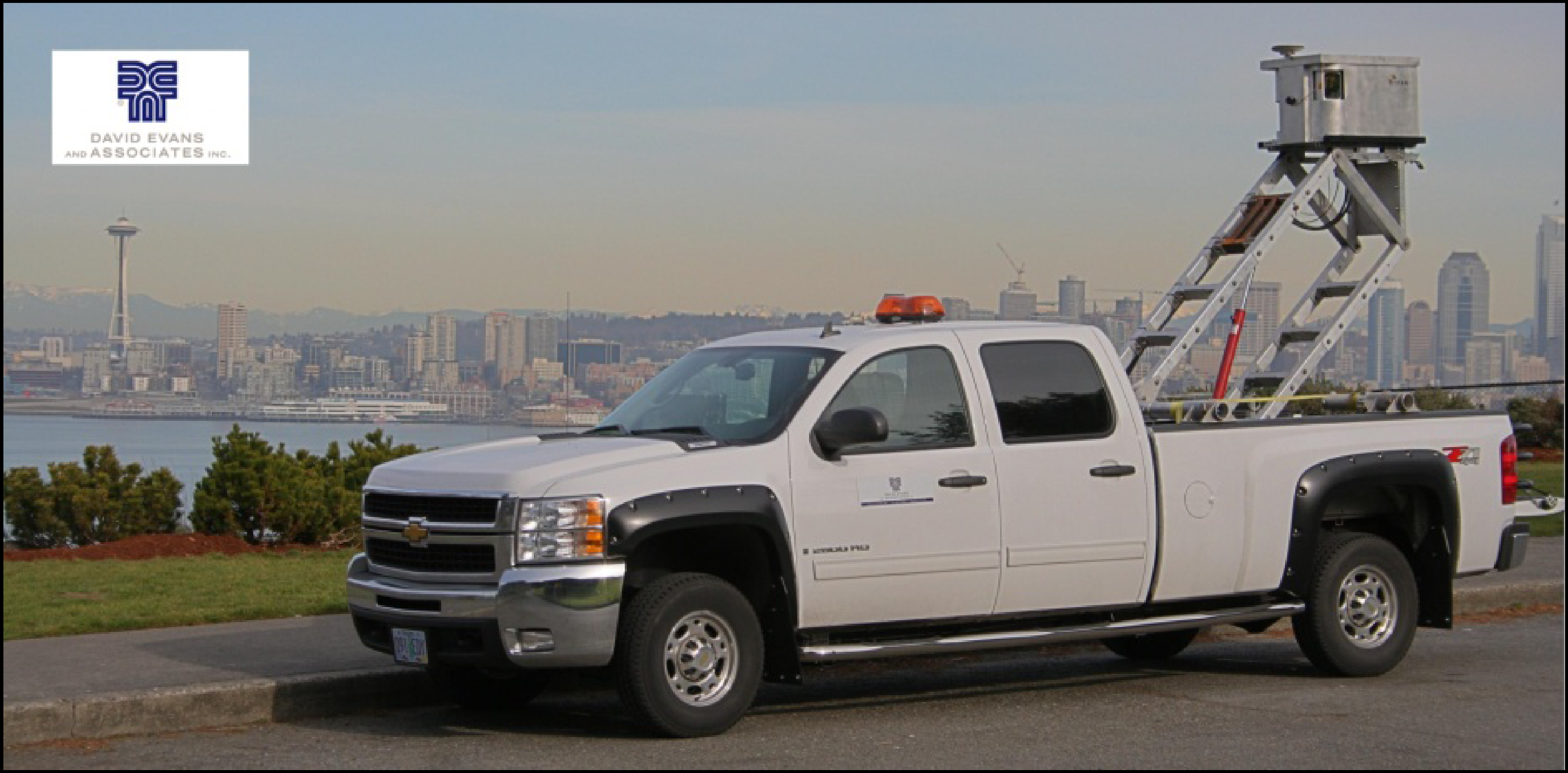
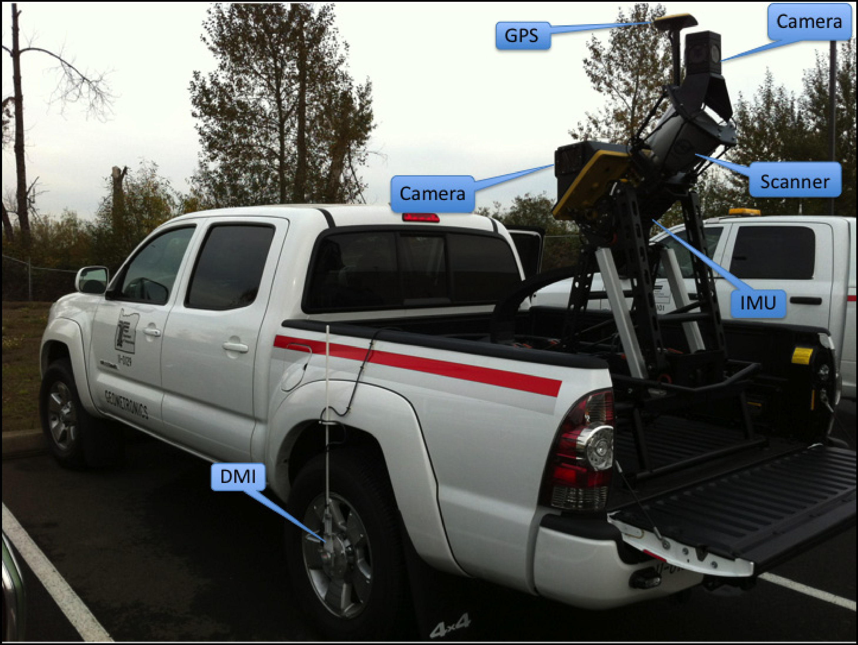

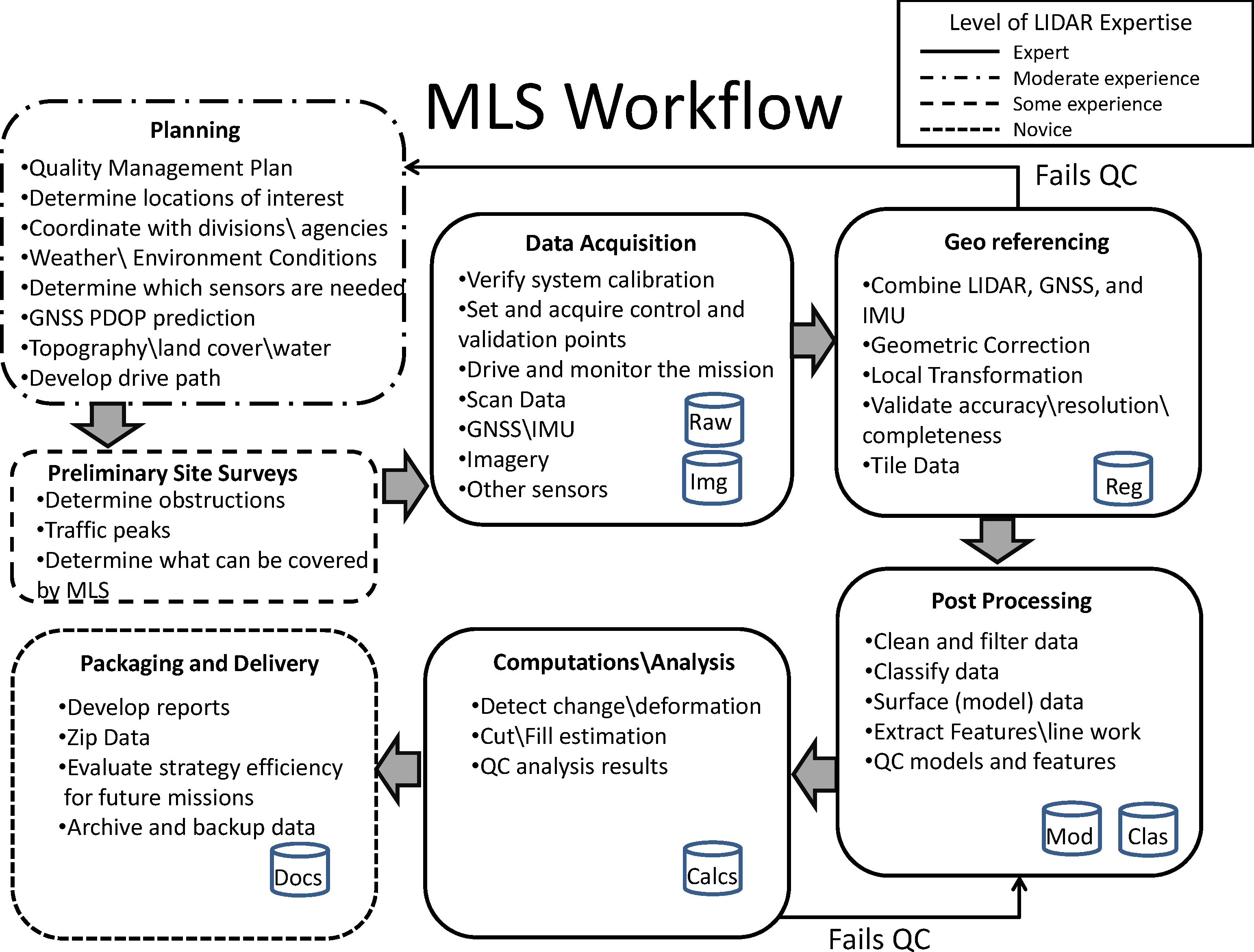


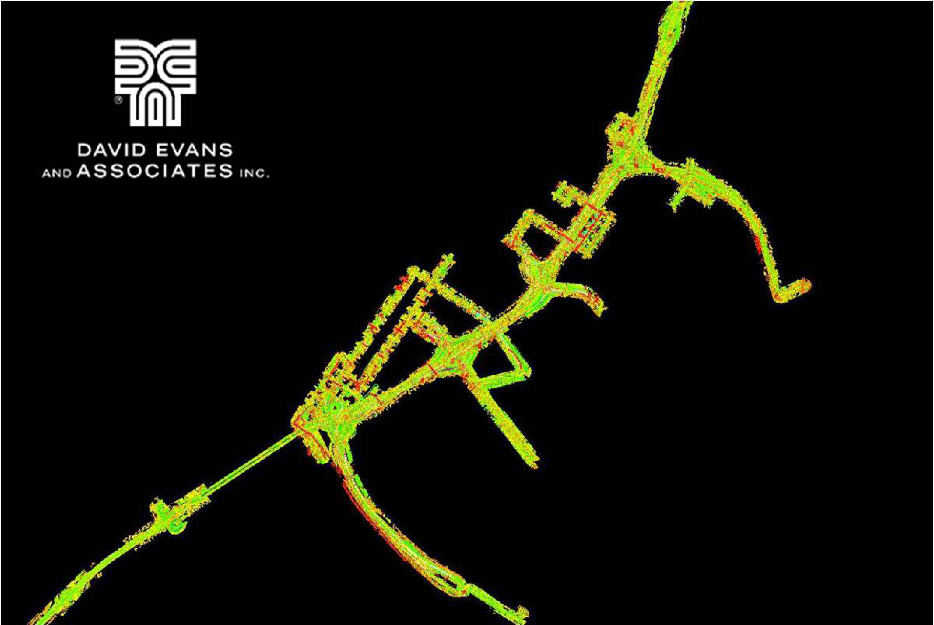
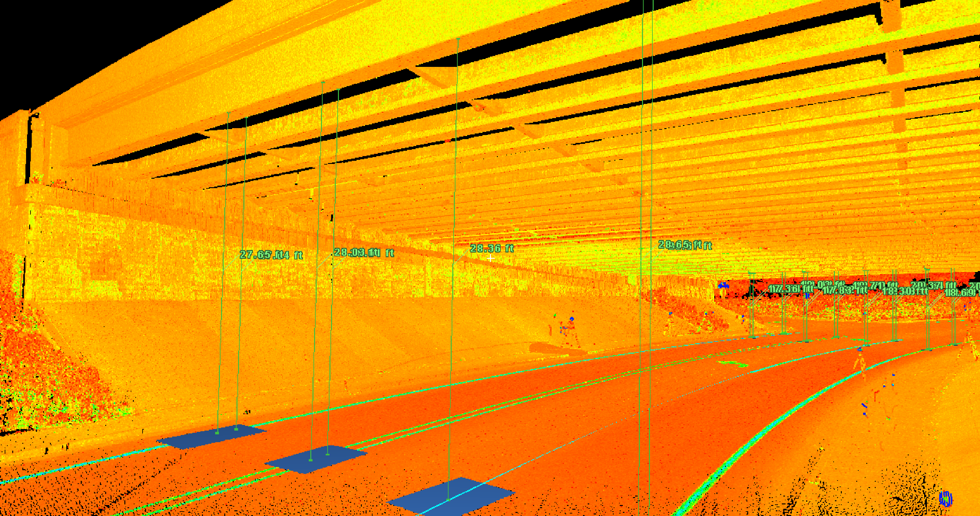


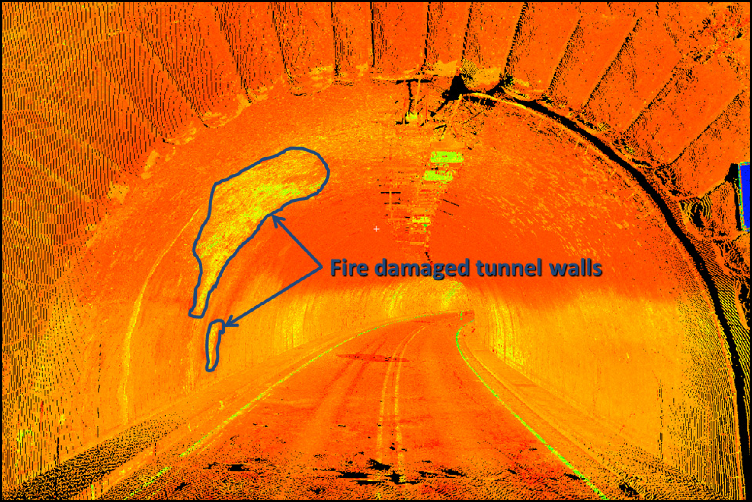
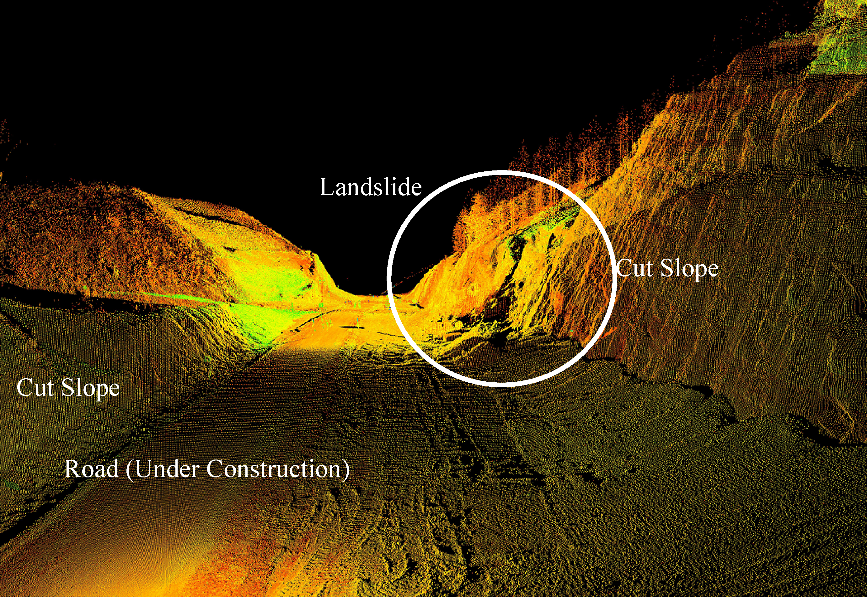
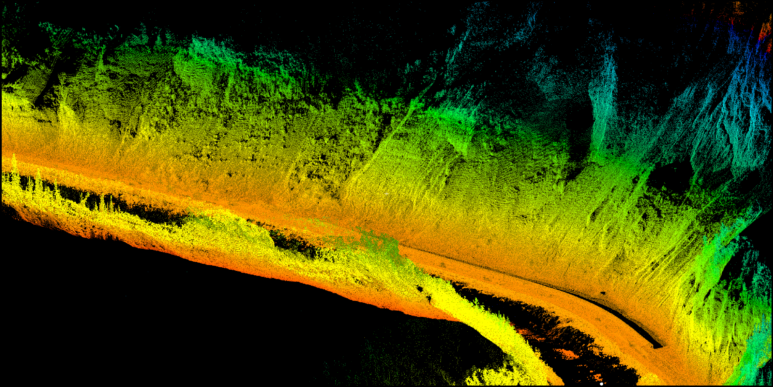
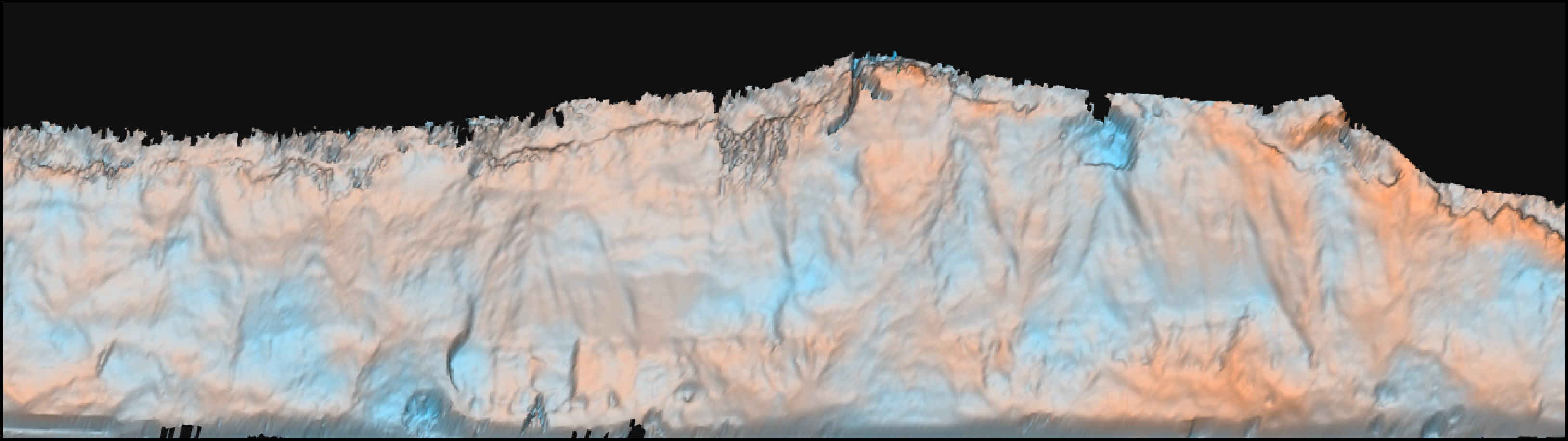
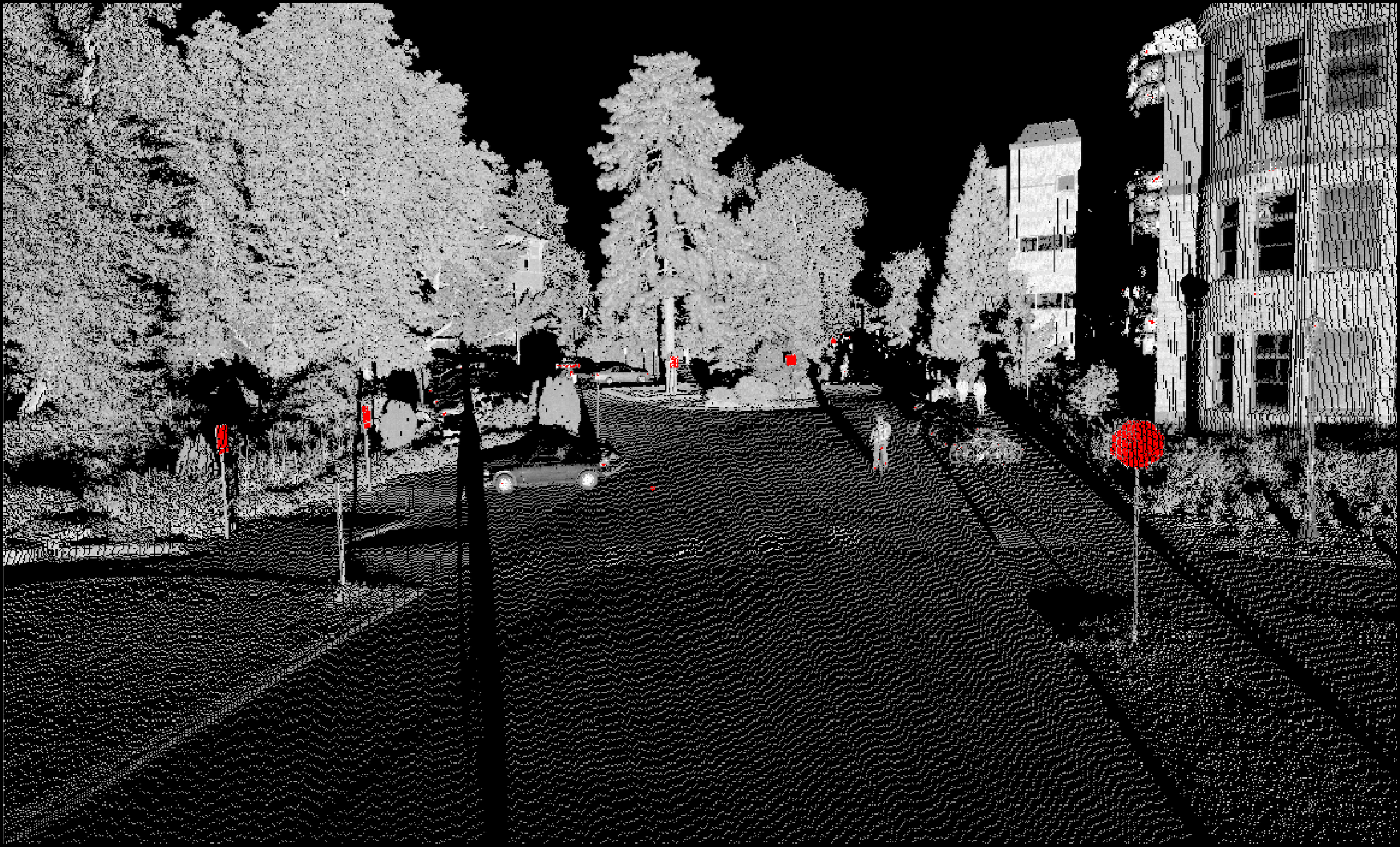

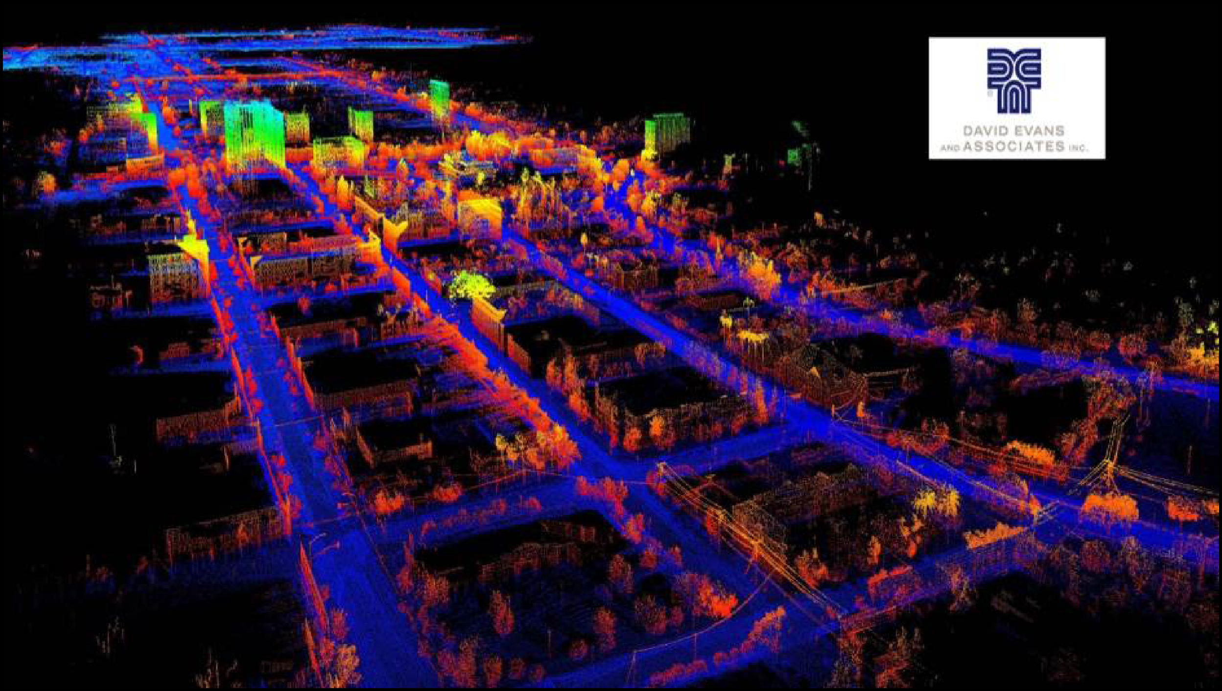
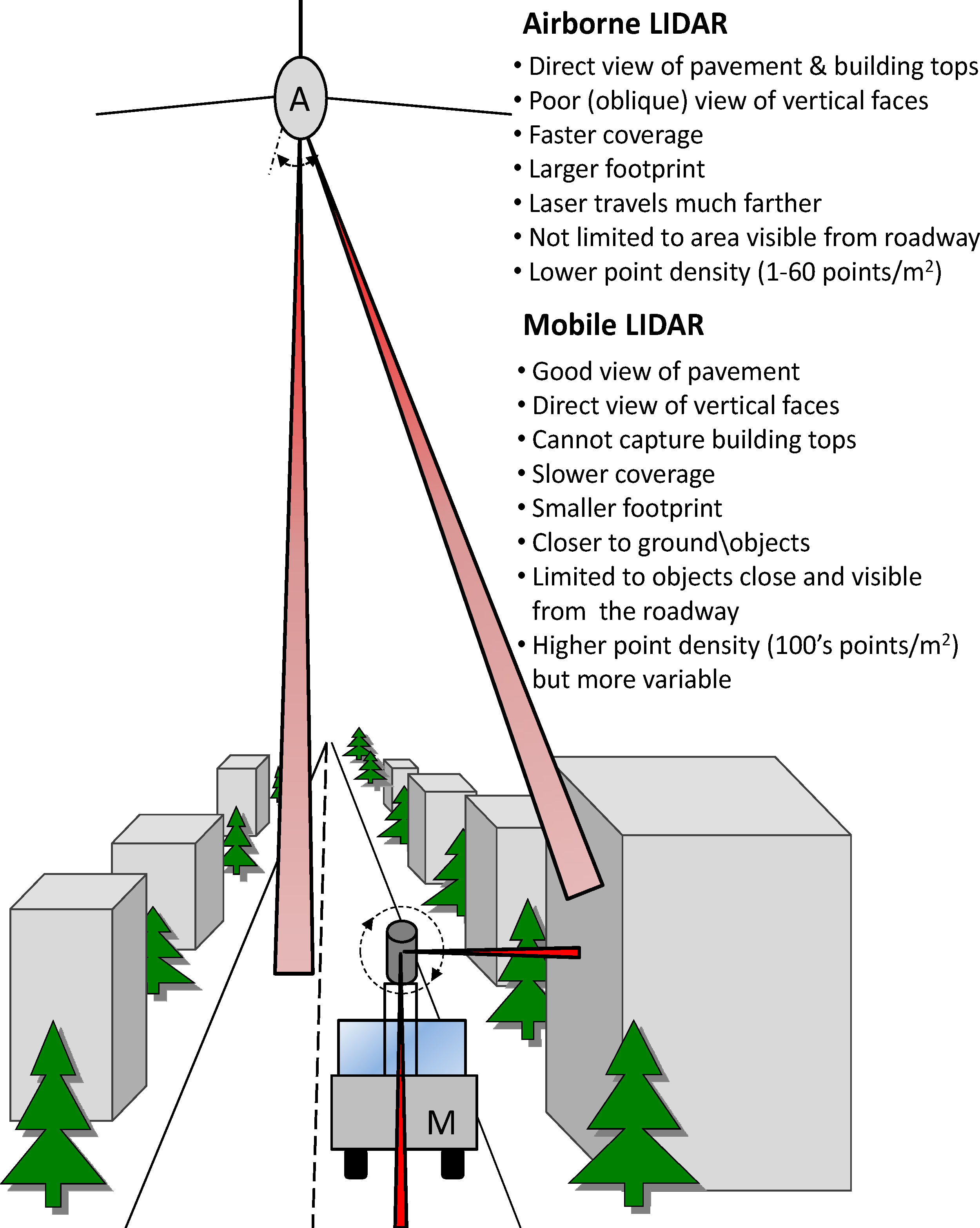
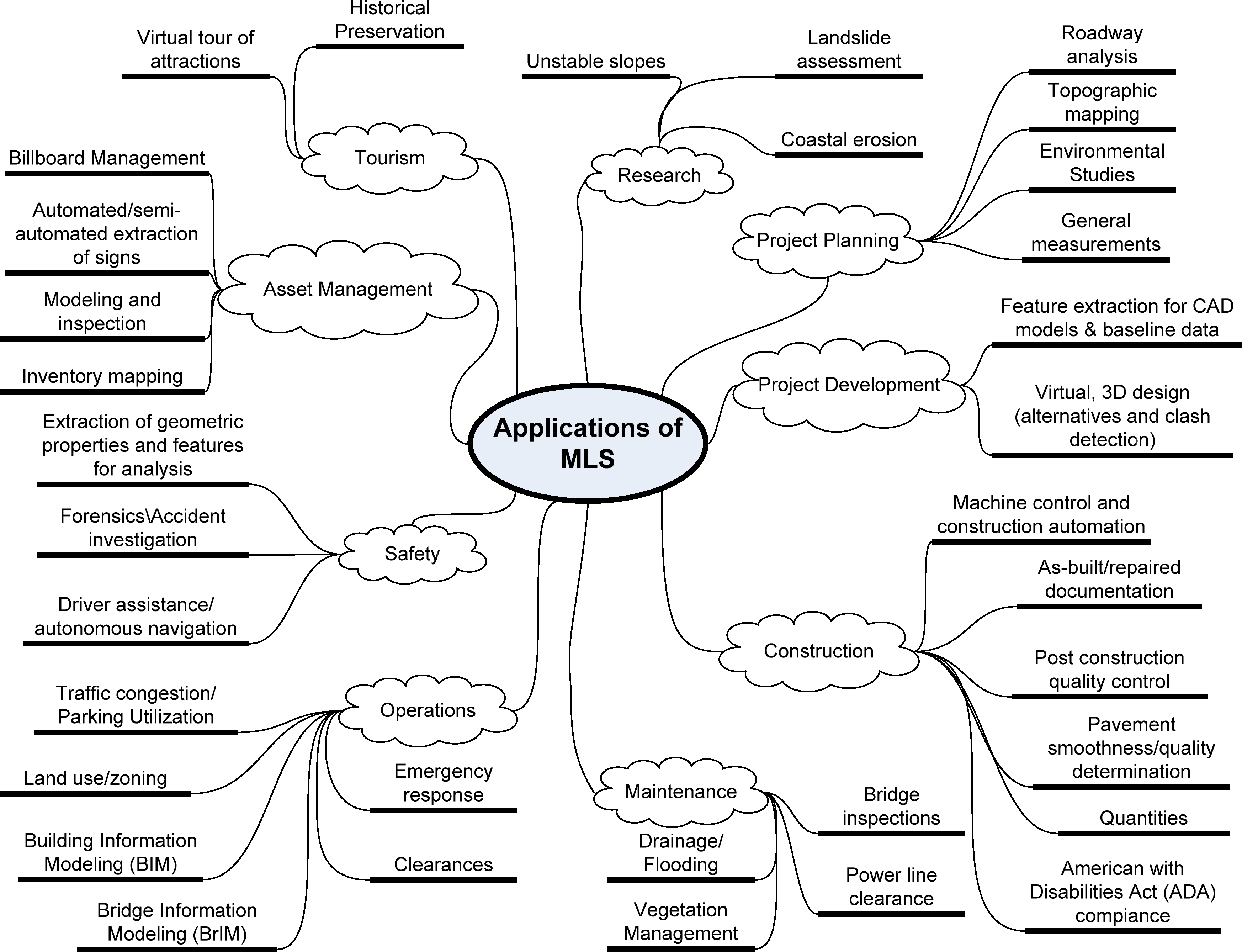
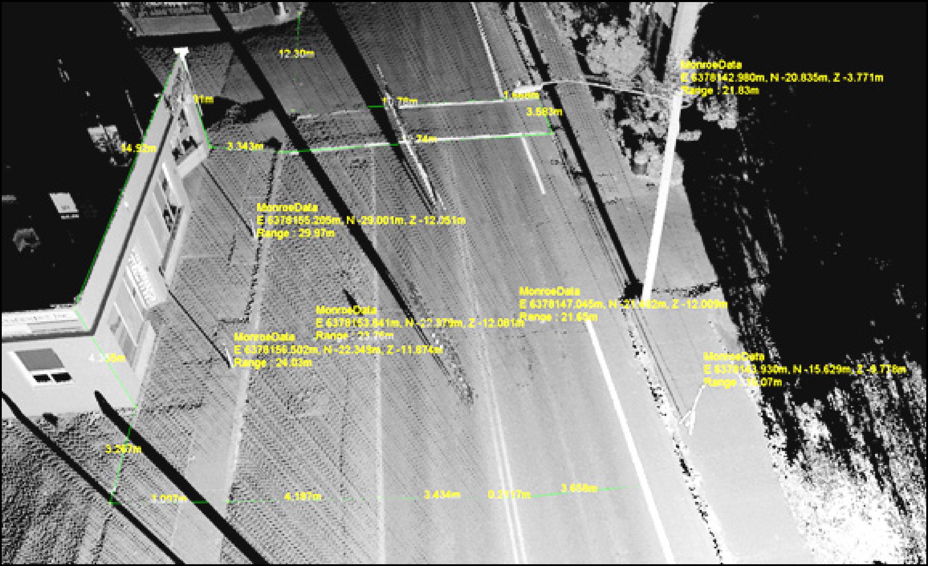
| Existing Guidelines | |
|---|---|
| General Geospatial | Key Points |
| Federal Geographic Data Committee (FGDC) 1996 National Standard for Spatial Data Accuracy (NSSDA) | 95% confidence evaluation, 20 control points, methodology on how to compute accuracy statistics |
| National Digital Elevation Plan (NDEP) 2004 | DTM certification, reporting of accuracy across many different remote sensing platforms. Discusses Fundamental, Supplemental, and Consolidated Vertical Accuracies (FVA, SVA, CVA) |
| Mobile LiDAR (Current) | |
| CALTRANS Chapt. 15 Survey Manual 2011 Florida DOT 2012 | TLS and MLS specifications, various classes of data (Type A-high accuracy, Type B-lower accuracy), requirements for: mission planning, control placement, system calibration, overlap requirements, QA/QC |
| NCHRP Report 748 (Olsen et al. 2013) | Guidelines for the use of mobile LIDAR for use in transportation applications. Focuses on accuracy (network and local) at 95% confidence levels as well as point density through the use of Data Collection Categories. The primary audiences of the document are management and staff who will be developing statements of work for MLS use in transportation. |
| Mobile LiDAR (Development) | |
| TxDOT | In development |
| ASPRS Mobile Mapping Committee | At outline stage |
| MoDOT 2010 | Evaluation of MLS usage for DOT activities |
| Airborne LiDAR | |
| FAA 2011 | Includes LIDAR (airborne, static, and Mobile) standards and recommended practices for airport surveys. System calibrations, data processing. |
| NOAA 2009 | Use of LIDAR for shoreline and flood mapping. |
| USGS (2012) | V1.0. Base Specification. Post spacing, overlap requirements, classification, metadata example, DEM., vertical accuracy assessment, glossary of terms. |
| ASPRS Vertical | Applying FGDC and NDEP guidelines to airborne LIDAR. Land cover types. Selection of checkpoints. |
| ASPRS Horizontal | Considerations (and difficulty) of horizontal accuracy verification. |
| ASPRS Geospatial Procurement Guidelines | Draft phase. Distinguishes between professional\ technical services and commercial geospatial products. |
| FEMA Guidelines | LIDAR use in floodplain mapping. |
© 2013 by the authors; licensee MDPI, Basel, Switzerland This article is an open access article distributed under the terms and conditions of the Creative Commons Attribution license ( http://creativecommons.org/licenses/by/3.0/).
Share and Cite
Williams, K.; Olsen, M.J.; Roe, G.V.; Glennie, C. Synthesis of Transportation Applications of Mobile LIDAR. Remote Sens. 2013, 5, 4652-4692. https://doi.org/10.3390/rs5094652
Williams K, Olsen MJ, Roe GV, Glennie C. Synthesis of Transportation Applications of Mobile LIDAR. Remote Sensing. 2013; 5(9):4652-4692. https://doi.org/10.3390/rs5094652
Chicago/Turabian StyleWilliams, Keith, Michael J. Olsen, Gene V. Roe, and Craig Glennie. 2013. "Synthesis of Transportation Applications of Mobile LIDAR" Remote Sensing 5, no. 9: 4652-4692. https://doi.org/10.3390/rs5094652
APA StyleWilliams, K., Olsen, M. J., Roe, G. V., & Glennie, C. (2013). Synthesis of Transportation Applications of Mobile LIDAR. Remote Sensing, 5(9), 4652-4692. https://doi.org/10.3390/rs5094652