Article

Estimating Riparian and Agricultural Actual Evapotranspiration by Reference Evapotranspiration and MODIS Enhanced Vegetation Index

1
Sonoran Desert Research Station, Southwest Biological Science Center, US Geological Survey, 1110 E. South Campus Drive, Room 123, Tucson, AZ 85721, USA
2
CSIRO Land and Water, Waite Road, Gate 4, Glen Osmund, SA 5064, Australia
3
Environmental Research Laboratory, University of Arizona, 2601 E. Airport Dr., Tucson, AZ 85706, USA
4
USDA-Agricultural Research Service, 2000 E. Allen Rd., Tucson, AZ 85719, USA
*
Author to whom correspondence should be addressed.
Remote Sens. 2013, 5(8), 3849-3871; https://doi.org/10.3390/rs5083849
Submission received: 26 June 2013 / Revised: 22 July 2013 / Accepted: 22 July 2013 / Published: 5 August 2013
(This article belongs to the Special Issue Advances in Remote Sensing of Crop Water Use Estimation)

Abstract

:
Dryland river basins frequently support both irrigated agriculture and riparian vegetation and remote sensing methods are needed to monitor water use by both crops and natural vegetation in irrigation districts. We developed an algorithm for estimating actual evapotranspiration (ETa) based on the Enhanced Vegetation Index (EVI) from the Moderate Resolution Imaging Spectrometer (MODIS) sensor on the EOS-1 Terra satellite and locally-derived measurements of reference crop ET (ETo). The algorithm was calibrated with five years of ETa data from three eddy covariance flux towers set in riparian plant associations on the upper San Pedro River, Arizona, supplemented with ETa data for alfalfa and cotton from the literature. The algorithm was based on an equation of the form ETa = ETo [a(1 − e−bEVI) − c], where the term (1 − e−bEVI) is derived from the Beer-Lambert Law to express light absorption by a canopy, with EVI replacing leaf area index as an estimate of the density of light-absorbing units. The resulting algorithm capably predicted ETa across riparian plants and crops (r2 = 0.73). It was then tested against water balance data for five irrigation districts and flux tower data for two riparian zones for which season-long or multi-year ETa data were available. Predictions were within 10% of measured results in each case, with a non-significant (P = 0.89) difference between mean measured and modeled ETa of 5.4% over all validation sites. Validation and calibration data sets were combined to present a final predictive equation for application across crops and riparian plant associations for monitoring individual irrigation districts or for conducting global water use assessments of mixed agricultural and riparian biomes.

1. Introduction

1.1. Need for Evapotranspiration Estimates for River Basin Irrigation Districts

Dryland (arid and semi-arid) agricultural districts are frequently located in riparian floodplains, using water diverted from the river for irrigation of crops. In these districts, crops and natural riparian vegetation often must co-exist on limited water supplies [1]. Riparian corridors provide habitat for fish, mammals and resident and migratory birds, while agriculture is the primary source of income for surrounding communities. Resource managers need accurate estimates of water requirements of both crops and riparian vegetation to construct district water budgets and apportion water. Globally, crop water budgets require robust algorithms that are calibrated for specific agricultural systems [2]. Irrigated lands account for about 18% of total cropland area but 40% of global food production. They also consume 60–90% of all water diverted for human purposes. Hence, the main goal of this study was to test the feasibility of developing a remote sensing algorithm for mixed riparian and crop systems in dryland irrigation districts that can be applied on a global basis.

1.2. Methods to Determine Crop Water Budgets

Several methods exist to estimate consumptive water use by crops. Often, diversions and drainages (return flows) are gauged to estimate each term [3]. Crop consumptive use (i.e., ETa) can then be estimated as a residual in a water balance equation. Another widely used approach is to census the planted fields within a district and to estimate consumptive use by applying a crop coefficient approach to the fields where:
ET a = K c ET o
where ETa is actual evapotranspiration, Kc is a crop coefficient and ETo is reference crop evapotranspiration estimated from meteorological data [3]. Kc is derived from experimental data for each crop and relates ETa to local meteorological conditions through ETo. An example of this approach is the Lower Colorado River Accounting System [4]. In well-monitored irrigation districts, ETo is calculated with data from local micrometeorological stations based on wind speed, relative humidity, temperature and net radiation data according to the FAO-56 formulation of the Penman-Monteith equation [5].
Water balance approaches can provide accurate data for closed basins over long time spans (typically annually or longer) over which changes in surface and groundwater storage are negligible compared to inflows and outflows. However, these conditions are not always met, and water balances are problematic over short time periods or for individual fields. Crop coefficient methods tend to overestimate crop consumptive use because they are typically derived for crops grown under optimal conditions in lysimeters, whereas actual field crops can have uneven stands and are subject to nutrient limitations and periodic water stress between irrigations. Also, neither of these approaches is easily adapted to riparian vegetation, for which crop coefficients might be variable or unknown.

1.3. Remote Sensing Methods for Estimating ETa

In response to these limitations, numerous methods have been developed to estimate ETa through remote sensing with satellite imagery [6,7]. These methods fall into two broad categories. Surface energy balance (SEB) methods use data from thermal infrared (TIR) satellite bands to estimate sensible heat flux, then calculate latent heat flux (ETa) as a residual in the SEB equation. By contrast, vegetation index (VI) methods, used in the present study, combine estimates of green foliage density with meteorological data to estimate evaporation from transpiring vegetation (Eveg). VI-ETo methods [810] substitute a VI for Kc in Equation (1) then calculate ETa based on locally-measured ETo:
E veg = aET o VI n
where a is a coefficient determined by regressing measured Eveg against a VI and n is an exponent relating Eveg to VI [11]. Sometimes Equation (2) is assumed to be a linear function, in which case n = 1. In some cases, as in the present study, the calibrating data come from measurements of ETa (e.g., from lysimeters or micrometeorological flux towers), in which case Equation (2) estimates ETa rather than Eveg.
Both SEB and VI methods have been reviewed recently, and their strengths and weaknesses compared [10,12,13]. Gonzalez-Dugo et al. [14] found similar levels of accuracy for SEB and VI-ETo methods compared to eddy covariance data in a mixed-crop, agricultural district in Iowa, subsequently adapting the later method to water-use monitoring in an irrigation district in Spain [15]. In this study, we tested the feasibility of developing a generalized VI-ETo algorithm that could be used to estimate ETa of arid-zone irrigation districts, including both crops and riparian vegetation. If successful, this algorithm could be used to characterize water use efficiency and crop and environmental water needs in this type of agricultural biome, as part of an overall strategy to assess global croplands water use [2].

1.4. Applicability of VI-ETo Methods to Dryland Irrigation Districts

The two main limitations of VI-ETo methods are: (1) they do not account for direct evaporation from flooded fields or from soil and canopies following rains; and (2) they do not account for short-term (periods of hours to several days) stress effects on plants [6,13]. These problems tend to be minimized in dryland irrigation districts where rainfall is infrequent and 80–90% of applied water is consumed in Eveg, see [5]. Stress of crops is minimized due to the provision of irrigation water, and riparian plants are mainly phreatophytes that have a more-or-less constant water supply from the shallow aquifer under the riparian floodplain [16] (also see [17,18]). Furthermore, an estimate of soil evaporation can be obtained separately with the two-source model for estimating ETa, which uses drying curves based on soil type to derive evaporation rates following an irrigation or rain event [19]. In districts with significant periods of wet soil due to rain or high-frequency irrigation (e.g., by overhead spray booms), the two-source model can be used [19]. However, in flood-and-furrow irrigated arid irrigation districts, the single-source model, which lumps evaporation and transpiration together in a single Kc, often performs nearly as well as the two-source model [3]. Moisture or nutrient stress can result in short-term decreases in stomatal conductance (GS), but in the longer term, plants tend to reduce leaf area index (LAI) to match the capacity of the environment to support photosynthesis [20]. Hence, over a crop cycle, stress results in a reduction in LAI which can be detected as a decrease in VI.

1.5. VI-ETo Methods Applied to Crops

Numerous studies have documented a strong correlation between VIs and crop ETa [10]. For example, the VI-ETo concept was tested for a number of crops in California’s Central Valley [21] and forms the basis of a prototype satellite irrigation management support system developed to predict real-time crop water demand in California irrigation districts [22]. Similarly, a recent set of experiments in Spain’s Guadalquivir basin irrigation district found an acceptable level of accuracy between ETa measured by eddy covariance flux towers and VI-ETo estimates of ETa for four test crops [14]. The authors concluded the VI-ETo method produced valid and robust estimates of ETa and they, too, developed an operational irrigation management program for farmers in the district based on spatially distributed ETa estimates from Landsat imagery [15]. Both methods had errors under 10% when compared to ground estimates of ETa. However, different algorithms were proposed for each irrigation district and no single VI-ETo method has yet been applied across a wide range of irrigation districts. Furthermore, riparian vegetation has not been included in estimates of irrigation district ETa. These methods can supplement more conventional water balance methods applied to irrigation districts in which not all the terms are adequately measured [23,24].

1.6. VI Methods Applied to Riparian Vegetation

Several studies have shown that riparian vegetation is also amendable to VI-ETo or other VI methods for estimation of ETa. Surface soils are typically dry for most of the year, so direct evaporation of water is low. Nagler et al. [25] developed an algorithm for riparian ETa based on the Enhanced Vegetation Index (EVI) from the Moderate Resolution Imaging Spectrometer (MODIS) sensor on the Terra satellite that adequately predicted (r2 = 0.74) ETa measured at eight moisture flux towers on three different river systems and over five different plant associations ranging from grasses to shrubs and trees. Scott et al. [26] found that this algorithm reproduced water balance estimates of ETa on the upper San Pedro River, Arizona, within 10%. Groeneveld et al. [16] found that a single summer Landsat Normalized Difference Vegetation Index (NDVI) image could be used to predict annual ETa measured at moisture flux towers for a variety of riparian and desert phreatophyte sites in the western US with r2 = 0.95.
Riparian plant communities are subject to environmental factors that can reduce ETa below ETo. ETa typically decreases with increasing depth to groundwater below about 2 m [27]. Depth to groundwater frequently increases over the summer as water is withdrawn to support ETa, hence ETa/ETo might not be constant over a growing season [28]. Furthermore, salts can accumulate in soils and aquifers, further limiting ETa [29]. Finally, soil hydraulic properties can constrain ETa by limiting the rate at which the capillary fringe from which phreatophytes extract water can be replenished during the day [30]. Nagler et al. [17,18], working at salinized sites on the Lower Colorado River, found that mean ETa across sites could be predicted by VI-ETo methods with a standard error of about 20% across sites, but that ETa at any given site could vary much more due to differences in aquifer and soil properties among sites.

1.7. Experimental Approach

Our overall goal was to develop a robust algorithm that could be used to estimate annual rates of water consumption by crops and riparian vegetation over entire irrigation districts. Our intention is to apply this algorithm, if successful, to assessing water use efficiency and pin-pointing opportunities for water savings in global irrigation districts [2]. However, ground data for ETa is often available only as short-term estimates over limited spatial areas. Furthermore, we wanted to develop an algorithm that could be applied over mixed vegetation districts, with crops and riparian plants of different roughness lengths and other biophysical properties. In this study, we developed an algorithm for ETa of mixed crop and riparian areas based on ETo and the EVI from the MODIS sensor on the NASA Terra satellite. MODIS images are acquired near-daily with 250 m resolution, hence are able to closely track the phenology of crops and riparian plants over a growing season. The algorithm was calibrated with eddy covariance flux tower data for riparian plant communities on the San Pedro River, Arizona, supplemented with data from cotton and alfalfa fields in southwestern irrigation districts. The algorithm was then tested against season-long results from seven irrigation districts or riparian zones in dryland areas in the US, Spain and Australia, determined by water balance or flux tower measurements as reported in the literature. We used seasonal or longer data sets for validation because the purpose of the algorithm is to predict season-long ETa, not just to reproduce short-term data as in the calibration set. Examples of the calibration and validation sites are shown in Figure 1.

2. Materials and Methods

2.1. Form of the Algorithm for ETa

The algorithm for ETa took the form used by Nagler et al. [25] and Guerschman et al. [31]:
ET a = ET o [ a ( 1 e ( bEVI ) ) c ]
where a, b and c are fitting coefficients and (1 − e(−bEVI)) is derived from the Beer-Lambert Law modified to predict absorption of light by a canopy [32]. As formulated for plant canopies, LAI normally replaces N in the Beer-Lambert equation as an estimate of density of light absorbing particles, and in our application EVI replaces LAI, assuming a linear relationship between EVI and LAI over LAI values from 0 to ca. 4 as demonstrated in [17,33]. The coefficient c accounts for the fact that EVI is not zero at zero ETa since bare soil has a low but positive EVI. Note that we are predicting ETa rather than Eveg with this equation because all our ground data sources for ETa included both Eveg and direct evaporation from soils. Ground data for ETa were used to determine the coefficients a, b and c by regression analyses.

2.2. Moisture Flux Tower Data

Riparian ETa data came from three eddy covariance moisture flux towers set in different plant communities on the upper San Pedro River, Arizona. The Charleston Mesquite (CM) tower (Figure 1A) was in a dense, mesquite woodland; the Lewis Springs Mesquite (LSM) tower was in a less-dense mesquite shrubland site; and the Lewis Spring Sacaton (LSS) tower was in a big sacaton grass (Sporobolus wrightii) site. Site details and procedures for measuring ETa and meteorological variables have been described in several previous publications listed below.
Scott et al. [34] described the woodland site in detail and documented the water and carbon dioxide fluxes measured in 2001 and 2002. Scott et al. [35] compared all three sites for water and carbon dioxide measurements made in 2003. This study includes these previously reported 2003 measurements plus an additional four years of data from each of these sites collected in 2004–2007. Scott et al. [34,35] gave details about the eddy covariance instrumentation and methods. Studies incorporating eddy covariance instrumentation commonly use the standard energy balance closure method to evaluate the accuracy and efficacy of their measurements [36]. The average daily closure ratio ([lE+H]/[Rn_G]) for the sites used in this study ranged annually from 0.89 to 0.92 for the woodland, 0.81 to 0.83 for the shrubland, and 0.76 to 0.78 for the grassland. These values are consistent with numerous other studies [36]. For our analysis we chose to follow Twine et al. [37] who suggested that forcing closure was justified when available energy was known and errors in its measurement modest. Consequently, we scaled our latent and sensible heat fluxes to force daily closure while conserving the measured Bowen ratio. We computed ETo as the evaporation which would occur from a short, well-watered grass with a fixed-height of 0.12 m following the FAO-56 method [5].

2.3. ETa and ETo of Selected Crops

The riparian vegetation in this study only covered the low end of possible ETa values based on ETo. The mesquite and grass plots in this study were not fully vegetated, with bare soil or sparse vegetation occurring between trees, and LAI tended to be lower than for agricultural crops. For example, typical woodland riparian zones on three river systems had ETa of only 40% of ETo [25]. We included literature values for alfalfa and cotton crops to cover the higher end of ETa values. One source of alfalfa ETa data was from Bowen ratio flux tower measurements made in a commercial, flood-irrigated, 30.1 ha alfalfa field in the Palo Verde Irrigation District (PVID) on the Lower Colorado River in 2007–2008 (Figure 1B) [38]. Alfalfa exhibited a saw-toothed pattern of ETa as it was cut approximately every 30 days in summer in the PVID. A single MODIS EVI pixel selected over the tower location was acquired for 16-day collection periods matched to ETa peaks in 2007 and 2008 (3 peaks per year). ETo was obtained from the Parker, AZ AZMET station in the same irrigation district [39].
A second source of alfalfa ETa data was from the Imperial Irrigation District (IID) in California, using ETa data collected at five commercial alfalfa farms over three years (2006–2008). ETa was measured by eddy covariance towers as reported in Hanson et al. [40]. ETo data was from the California Irrigation Management System (CIMIS) [41]. MODIS EVI pixels were acquired for the period 2006–2008, and mean annual ETa across sites was correlated with mean annual EVI across sites. The exact location of the commercial fields was not given in [40] so we chose five fields identified as alfalfa fields by having year-round high EVI exhibiting the characteristic sawtooth patterns due to cutting. Hence, the fields we chose were not necessarily the same fields where flux towers were located but both data sets represented commercial fields within the IID.
Cotton ETa values were obtained from the USDA-ARS Conservation & Production Research Laboratory, Bushland, Texas [42]. ETa data were collected in a 10 ha field planted to cotton in 2008 as part of an experiment to compare lysimeter ETa values with those collected by neutron hydroprobe soil water balance and eddy covariance flux towers (Figure 1C). Two precision weighing lysimeters (9 m2 each) in the field were surrounded by cotton planted at the same density and irrigated at the same frequency as the lysimeter crops. We obtained the MODIS EVI pixel centered on the middle of the field for the dates of maximum ETa and LAI (DOY 219-247) using neutron probe results as they were distributed over the whole field. ETo data was from an on-site micrometeorological station and was calculated by the FAO-56 method [5].

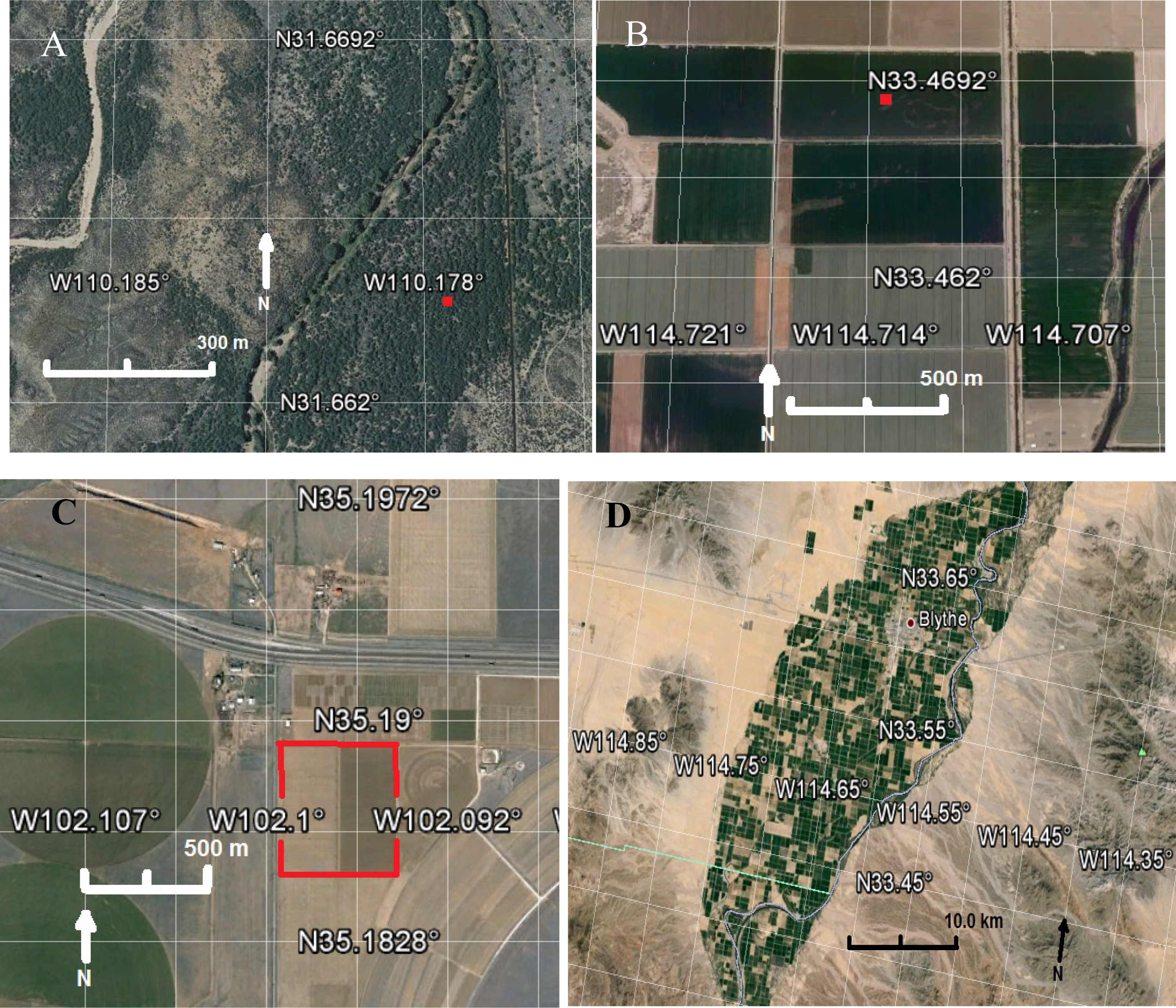
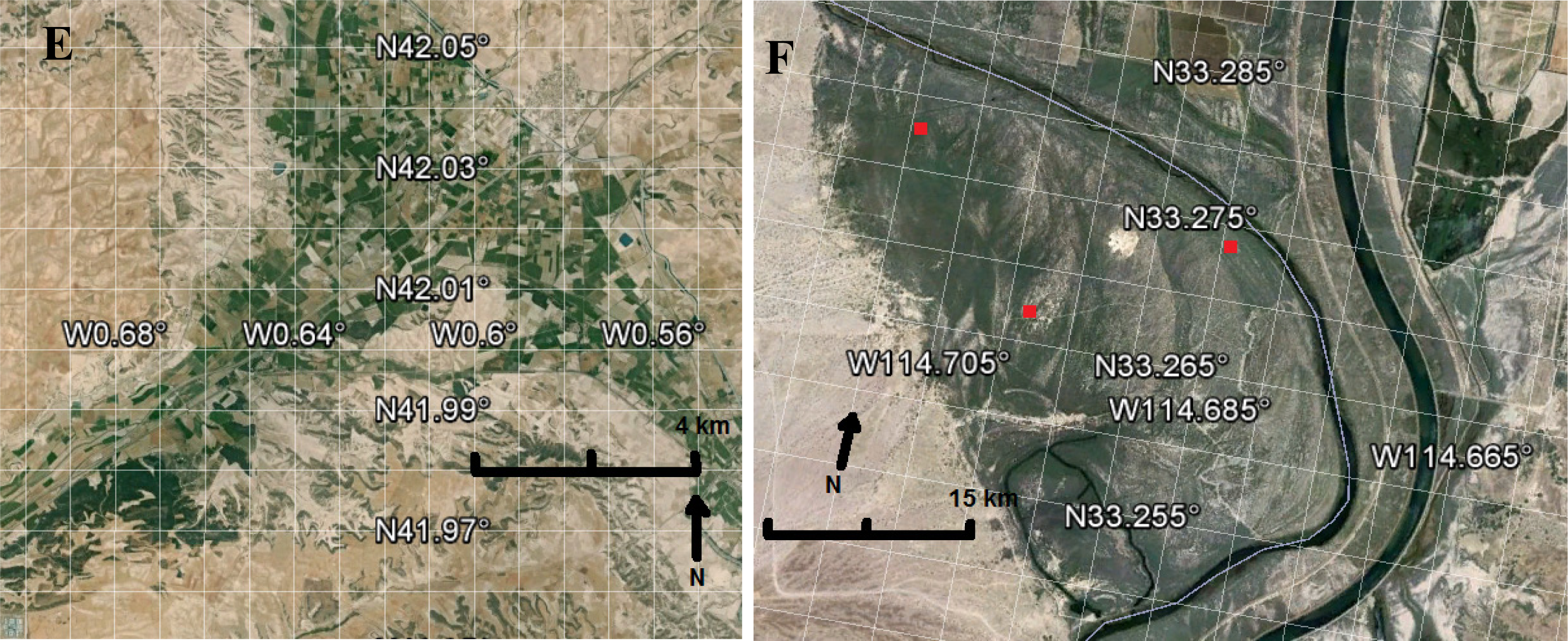
2.4. Sources of Validation Data

We tested the ETa algorithm against annual data collected for five dryland irrigation districts and two riparian areas based on independent estimates of ETa not included in the calibration data sets (Table 1). Crop ETa estimates were based on water balance estimates over one or more growing seasons, in which ETa was reported as a residual of inflows minus outflows. Taghvaeian and Neale [43] constructed a water balance for the PVID for 2008 (Figure 1D), using gauged inflow and outflows and estimates of canal losses and seepage generated by the irrigation district. Cultivation is year-round and the main crops are alfalfa, cotton, small grains and winter vegetables. Their estimate for ETa was 1,268 mm·yr−1. We obtained MODIS EVI pixels for the dates covered in the water balance study but created a 500 m buffer zone to exclude MODIS pixels that were mixed with adjacent desert habitat. ETa estimated by MODIS was then compared to ETa by the water balance study.
Allen et al. [3] conducted a detailed water balance for IID for the period 1990–1996 based on gauged inflow and outflow data and a census of planted areas. Most of the IID has a subsurface drainage system through which the drainage fraction is collected and conveyed to the Salton Sea for disposal; hence all outflows can be quantified. Reference evapotranspiration (ETo) is monitored at three stations in the district [41]. Over 40 different crops are grown in IID including alfalfa, cotton, sugar beets, corn, wheat, Sudan grass, Bermuda grass and winter vegetables. They reported ETa of 1,243 mm·yr−1. We updated their estimate to 2001, the first complete year for which MODIS imagery was available, using consumptive water use data from the Lower Colorado River Accounting System [44]. They reported diversions minus returns of 3.61 × 10⁹ m3·yr−1 for 2001, equal to 1,763 mm·yr−1 over the 2.16 × 10⁵ ha cropping area as reported in [3]. However, returns did not include flows to the Salton Sea from subsurface drainage in IID, estimated at 1.23 × 10⁹ m3·yr−1 [45] and yielding an ETa estimate of 1,194 mm·yr−1, close to the more detailed estimates in Allen et al. [3] for 1990–1996. We compared this estimate to a MODIS ETa estimate for 2001 obtained by acquiring pixels incorporating the IID minus a buffer zone around the perimeter of the district.
Greenwood et al. [46] conducted a water balance study of maize under center-pivot irrigation in a 30.4 ha field in Northern Victoria, Australia (VAU). They measured crop water use over two growing seasons (2003–2005) based on measured application rates and soil moisture depletion rates measured weekly by neutron hydroprobe. Mean ETa was 666 mm·yr−1 over both growing seasons (ca. 150 days each). We acquired data for the single MODIS EVI pixel located over the center of the field for the dates over which crop ETa was estimated by Greenwood et al. [46].
Lecina et al. [47] conducted a water balance study of the Bear River Irrigation Project (BRIP), Utah, for the 2008 growing season over a 1,213 ha surface irrigated area in which on-farm measurements of irrigation applied and infiltration were made at 13 sites over the season. Main crops are alfalfa and other forages, corn and winter/spring cereals. Mean ETa was estimated to be 877 mm for the April to October irrigation season. MODIS EVI pixels covering the dates of the water balance study were acquired for the study area minus a buffer zone. Barros et al. [23,24] conducted a water balance study in La Violada Irrigation District (LVSP) (4,000 ha) (Figure 1 E) in the Ebro River Basin in Spain for the years 1995–2008. The balance was based on measured diversions and returns and estimates of ETa based on soil moisture depletion rates following irrigation events. Main crops are corn, alfalfa and winter cereals. ETa for 2001–2008 (the period for which MODIS imagery was available) was 616 mm·yr−1. We obtained the MODIS EVI pixels encompassing the area of LVSP minus a buffer area around the perimeter for model evaluation.
The final validation included data for two riparian areas within irrigation districts: The Cibola National Wildlife Refuge (CNWR), a saltcedar (Tamarix ramosissima) dominated terrace on the Lower Colorado River below PVID (Figure 1F), and a site on the Platte River dominated by common reed (Phragmites australis). At the first site, ETa was measured at three Bowen ratio moisture flux towers set in stands of saltcedar chosen to represent the range of conditions on the terrace in 2007 and 2008 [38]. Mean ETa over sites and years was 817 mm·yr−1. Corresponding MODIS EVI pixels were acquired to encompass the CNWR minus a buffer area around the perimeter. Irmak et al. [48] measured ETa with a Bowen ratio moisture flux tower in 2009 and 2010 at a site on the Platte River dominated by common reed (Phragmites australis) and surrounded by rain-fed and irrigated crops in Merrick County, Nebraska (PR). Mean ETa of the riparian vegetation over the two years was 379 mm·yr−1. We acquired the single MODIS EVI pixel centered on the tower site for the dates covered by the tower ETa measurements.

2.5. Acquisition of MODIS EVI Pixels

MODIS MOD 13 gridded 250 m VI products are supplied to end-users by NASA as atmospherically and radiometrically corrected 16-day composite images (for details of image acquisition and processing see: http://modis.gsfc.nasa.gov/); MODIS EVI pixels were obtained from the Oak Ridge National Laboratory [49]. The pixel selection tool displays the approximate MODIS pixel footprint on a high-resolution Google Earth image; hence it is possible to positively co-locate ground sites with pixel acquisition sites if images or maps are available for the ground site locations. This condition was met for all sites except the IID alfalfa sites in this study. The choice of EVI was based on its superior performance in predicting ETa noted in previous studies [6,25]. EVI is calculated from band reflectance values as:
EVI = 2.5 × ( NIR Red ) / ( 1 + NIR + ( 6 × Red 7.5 × Blue ) )
where the coefficient “1” accounts for canopy background scattering and the blue and red coefficients, 6 and 7.5, minimize residual aerosol variations [6].

2.6. Statistical Analyses and Other Methods

Statistical and graphical analyses were conducted with Systat, Inc., software (SigmPlot 12.5), Chicago, IL Exponential curves and linear regression equations were fit to data points by the least squares method, and goodness of fit is reported as the coefficient of determination (r2), standard error of means (SEM) and P-value for the regression coefficient (slope) of each equation. ETa estimates by MODIS were compared to ground estimates by the t-test for paired values. Since 6 of 7 ETa estimates were lower by MODIS compared to ground methods, potential bias was also assessed by the Wilcoxon Signed-Rank test using an on-line calculator ( http://www.vassarstats.net/wilcoxon.html).

3. Results and Discussion

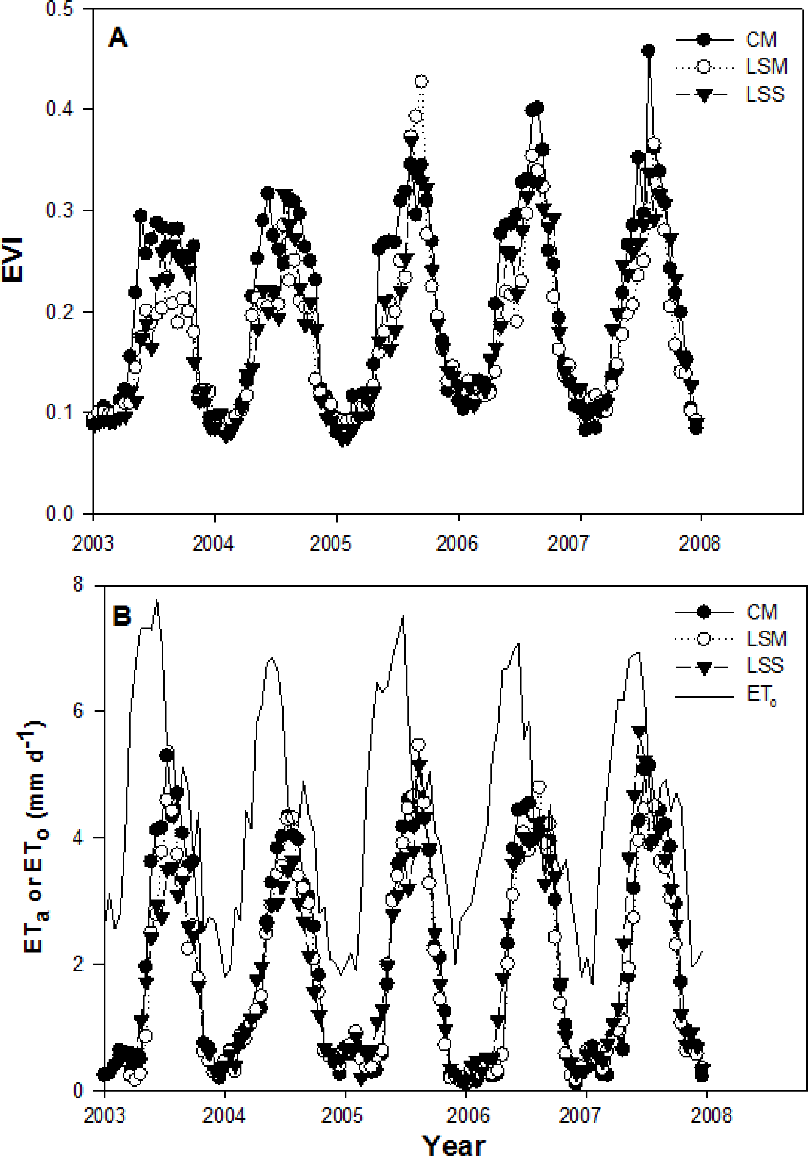
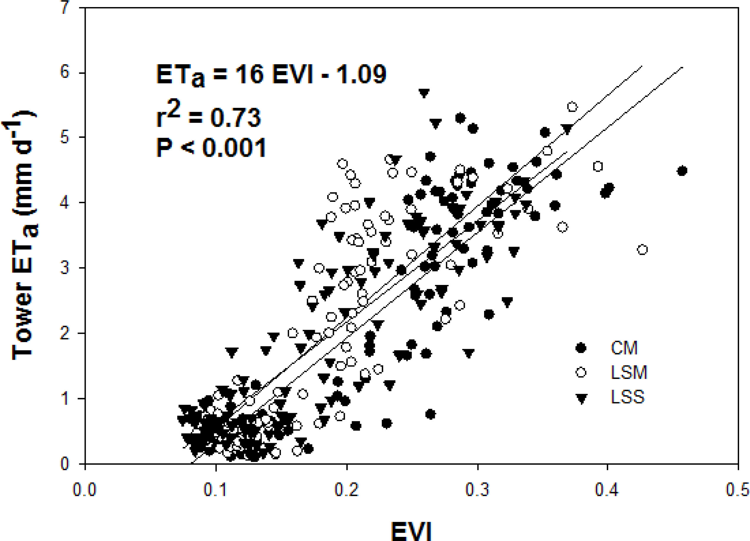
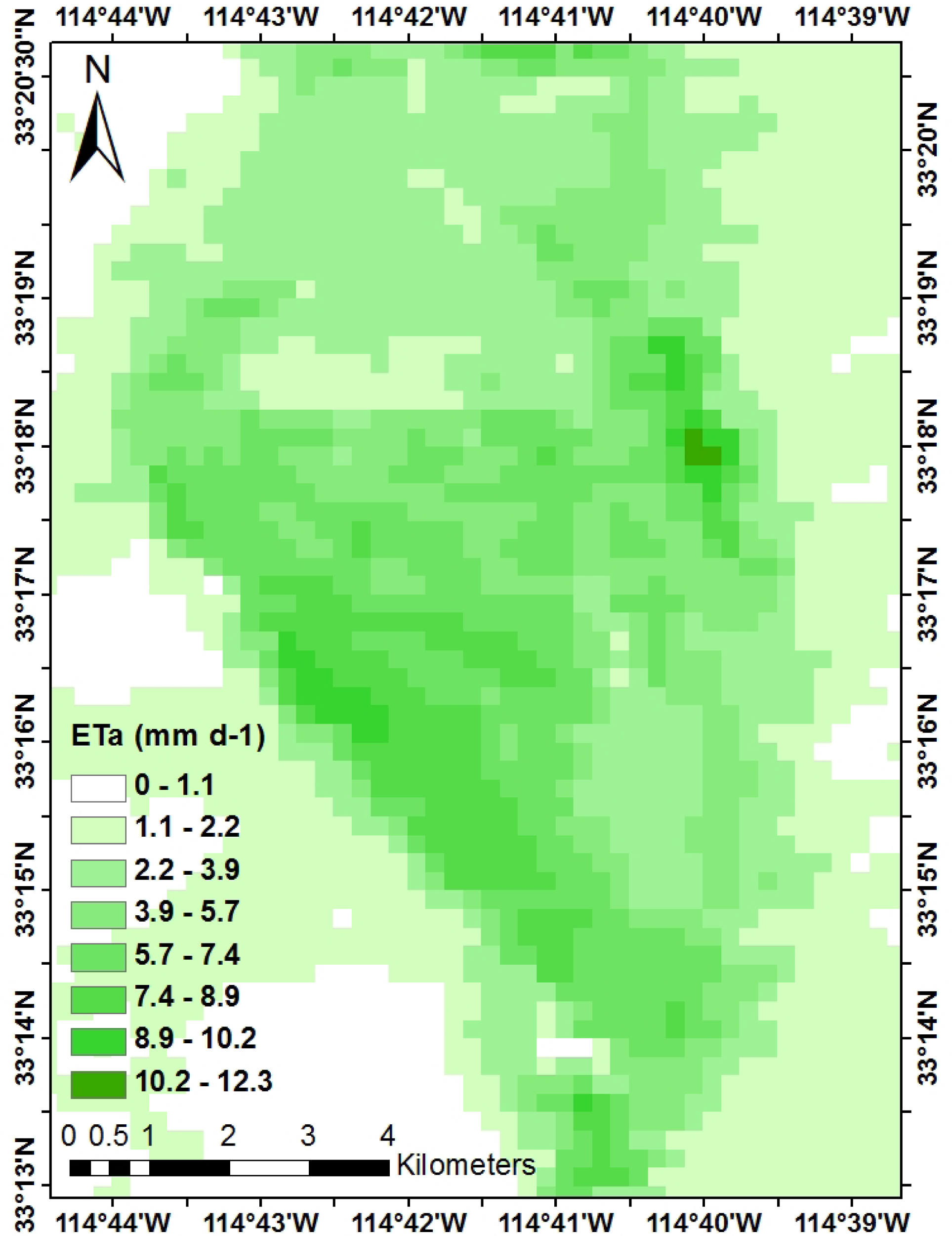
3.1 EVI and ETa Data for San Pedro Riparian Vegetation

Sixteen-day time-series of EVI are shown in Figure 2A and ETa at each tower are compared to ETo in Figure 2B. Peak summer EVI and ETa values tended to overlap among sites. Peak ETa values were about 60% of ETo, and were only 42% of ETo on an annual basis, as the vegetation was dormant during winter. ETa lagged behind ETo, with peaks in July vs. June, respectively. ETa was strongly correlated with EVI across sites (Figure 3), and slopes of ETavs. EVI were not significantly different at the 95% confidence level (P > 0.05) among sites.

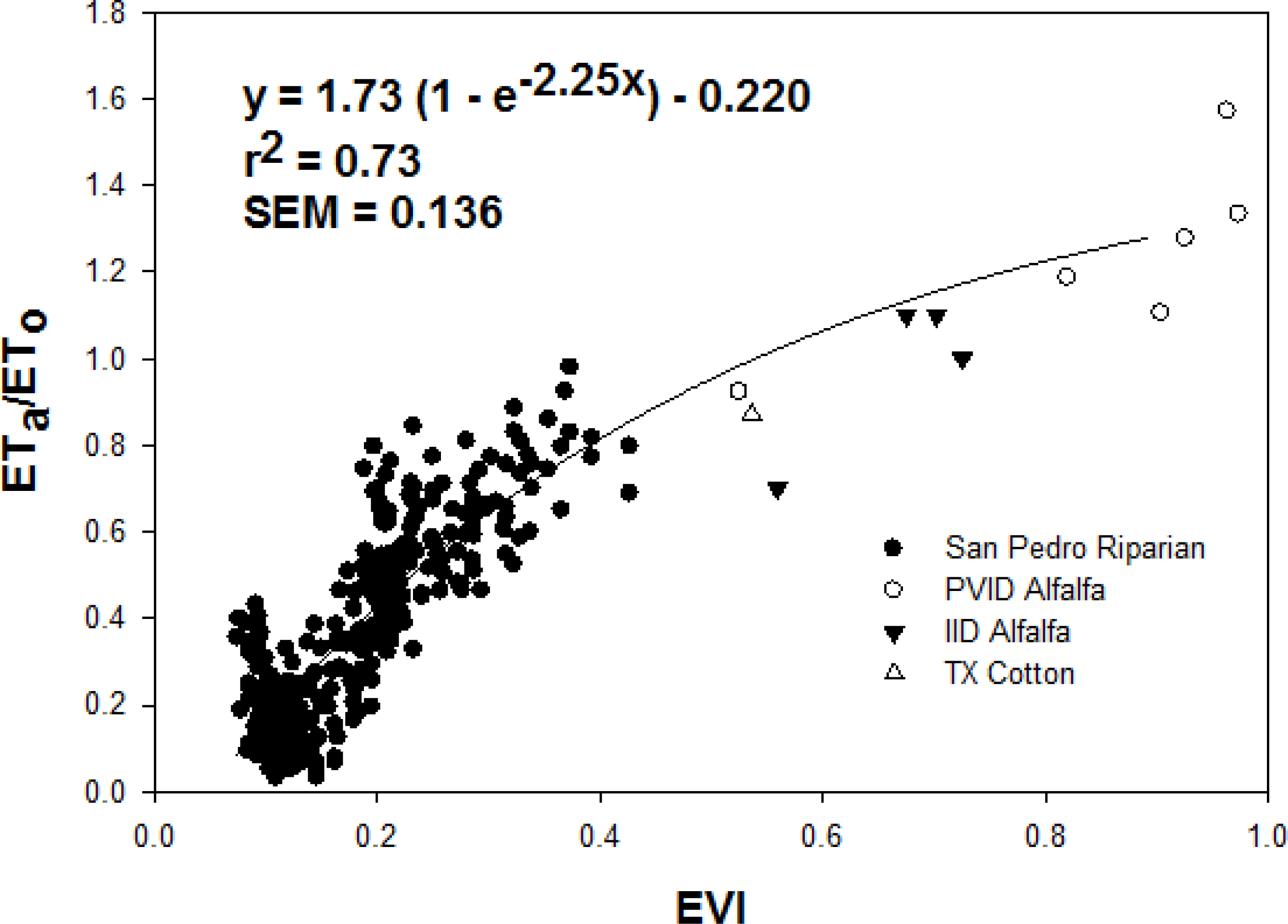
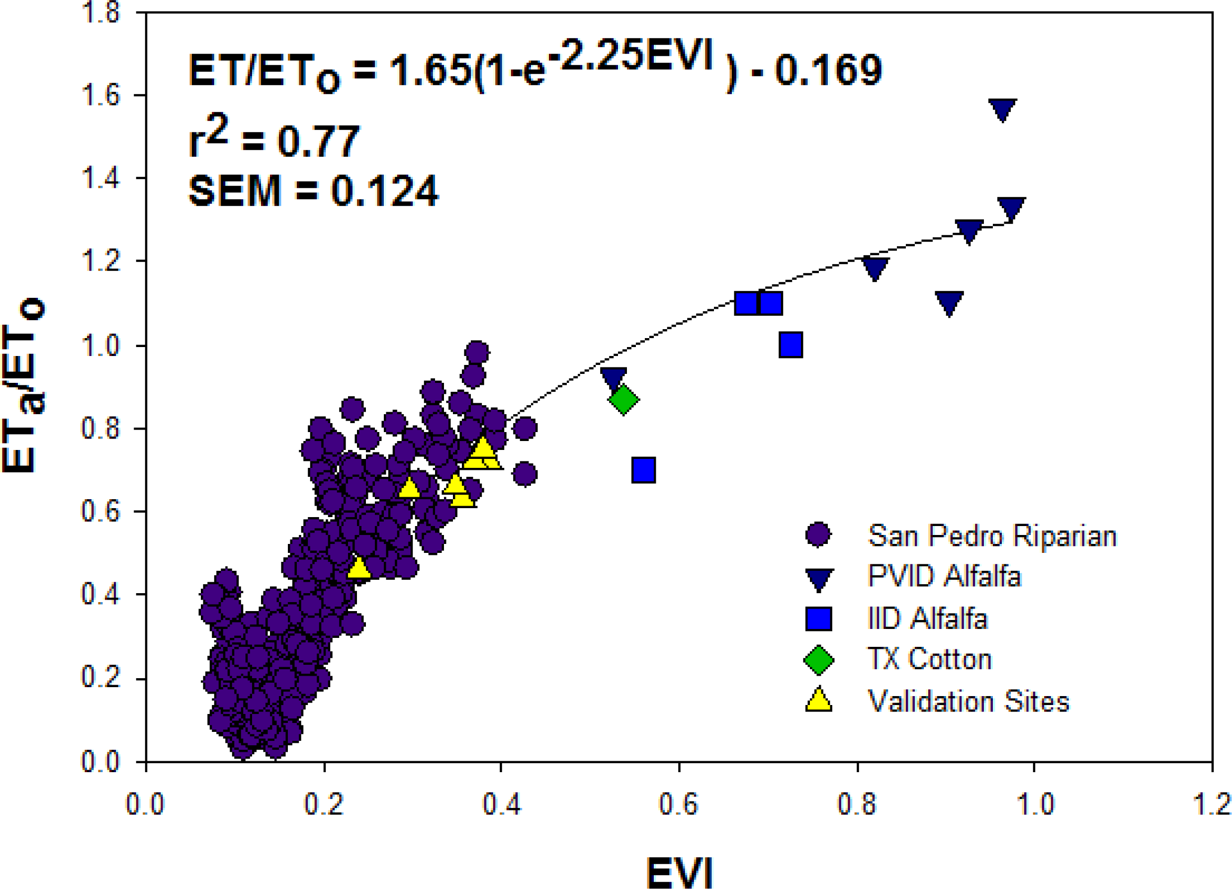
3.2. EVI vs. ETa/ETo for Combined Riparian and Crop Sites

Since ETo differs among irrigation districts due to local meteorological conditions, ETa was normalized as ETa/ETo across combined sites (Figure 4). ETa/ETo increased with EVI but was distinctly nonlinear. An algorithm in the form of Equation (3) fit the data with r2 = 0.73 and a standard error of the mean (SEM) of 0.136 of ETa/ETo. Maximum ETa/ETo projected for EVI = 1.0 is 1.29, within the range expected for freely transpiring alfalfa crops compared to grass reference crop ETo [3,5]. On the other hand, a linear model would greatly overestimate ETa/ETo if based on riparian data, and would underestimate riparian ETa/ETo if based on crop data. Therefore, Equation (5), which has a biophysical justification based on the Beer-Lambert Law, succeeds in unifying riparian and crop data into a single algorithm:
ET a = ET o [ 1.73 ( 1 e 2.25 EVI ) 0.220 ]

3.3. Validation Data Sets

Estimates of ETa by MODIS EVI using Equation (5) are compared to ground estimates of ETa in Table 1. Differences between estimates for individual sites ranged from 2.9 to 9.7% and the difference between means across all sites was 5.4%. Individual site differences were not significant by paired t-test (P = 0.894). However, ETa at 6 of 7 sites was higher by MODIS than by ground estimates, a marginally significant difference (P = 0.051) by the Wilcoxon Signed-Rank test (W = 24), indicating a possible small positive bias for the MODIS estimates compared to the ground estimates.

3.4. Final Equation for ETa

Since ETa across sites did not differ significantly between methods for the validation data, they were combined with the calibration data to produce a final equation of best fit (Figure 5). The r2 (0.77) and SEM (0.124) improved slightly compared to calibration data (Figure 4). The final equation of best fit was:
ET a = ET o [ 1.65 ( 1 e 2.25 EVI ) 0.169 ]
The projected ETa/ETo at EVI = 1.0 was 1.29. Hence, ETa was constrained between 0 at EVI = 0.05 (e.g., bare soil or dormant vegetation) and 1.28 ETo at EVI = 0.973, the highest EVI value observed in this study. Nagler et al. [18] developed a preliminary algorithm for ETa for agricultural and riparian associations on the Lower Colorado River, using a limited data set and a linear regression model. Equation (6) should provide more accurate predictions over a wider range of ETa than the previous algorithm.
ETa maps of the Palo Verde Irrigation District agricultural fields and the Cibola National Wildlife Refuge riparian zone are displayed in Figures 6 and 7, respectively. These maps are based on three MODIS collection periods in June and July 2007, during the period of ground ETa measurements by Bowen ratio flux towers. The maps show the general features of ETa within each area, but due to the low resolution of MODIS imagery, they could not capture the distribution of ETa within individual fields and could not be used for tasks such as irrigation scheduling on specific farms.

3.5. Limitations and Sources of Error and Uncertainty in ETo and ETa Estimates

Despite the apparent success of Equations (5) and (6) in predicting ETa across crops and riparian vegetation, some caveats must be considered. First, the ground data used to calibrate and validate remote sensing methods are themselves subject to error and uncertainty. For example, the source of ETo data can produce error among estimates [50]. While all of the present results were based on ETo calculated for a hypothetical grass reference crop by the FAO-56 method [5], the required data are not available for all irrigation districts on a global basis and are rarely available for riparian corridors away from irrigation districts. Simpler methods of calculating ETo, for example from temperature or solar radiation data, are available, but they can differ from the FAO-56 method by 10% or more and can exhibit different seasonal patterns [50]. The FAO-56 method is specifically designed for short crops with radiation as the main constraint on ETo and might not be the best scalar for tall crops or natural vegetation units, e.g., [18]. Furthermore, ETo is subject to measurement error. Allen et al. [3] pointed out that the CIMIS system replaced measurements of net radiation with estimates based on solar radiation in 1989, resulting in a 13% lowering of ETo values at IID after the change in methods, a discrepancy which has not been corrected. ETo estimates by CIMIS and AZMET stations in the same irrigation districts along the Arizona-California border also differ by about 11% (higher by AZMET) [51].
Ground methods for measuring ETa are also subject to error. Lysimetry is perhaps the most accurate way to measure ETa, with errors under 5% [52] but extrapolating lysimeter results to field conditions can produce errors in the order of 10–20% even under controlled conditions [42]. Water budget methods for estimating ETa typically have error rates of 5–10% even under ideal conditions, and the error rates increase when some of the terms have to be estimated rather than measured. Allen et al. [52] estimated that Bowen ratio and eddy covariance moisture flux towers have typical errors in the order of 15–30%, which can perhaps be reduced to 10–15% under ideal conditions. In the present study, the SEM for the calibrating data set was about 23% of the mean value of ETa/ETo, and the SEM for the combined validation and calibration data sets was 21%, within the error bounds of the likely ground measurement errors. However, the average error for predicting ETa/ETo by Equation (5) was less than 10% for each individual validation site and was only 5.4% across sites. This suggests that errors are likely to be random rather than systematic, so the SEM decreases as more sites and longer measurement periods are added [53].

3.6. Comparison with Other VI Methods for ETa

Several remote sensing methods have been developed recently to estimate ETa with VIs or other optical band combinations (i.e., surface reflectance in visible + NIR bands, in contrast to SEB methods that use TIR bands). VI methods cannot be used to measure instantaneous rates of ETa as can thermal band methods, but for long-term monitoring of ETa, this is an advantage because VI values tend to be stable over days to weeks, while thermal bands provide only a snapshot of the SEB at the time over satellite overpass. We briefly review three remote sensing methods below to show the basic similarities in approach and levels of accuracy of these types of methods.
Guerschman et al. [31] developed a procedure for estimating ETa at the continental scale in Australia. It was based on MODIS EVI in the same exponential-decay, rise-to-a-maximum form as in Equation (3), but it also used the Global Vegetation Moisture Index (GVMI) as a means to differentiate between open water and bare soil when EVI is low. The GVMI detects water by absorption in the short wave bands on MODIS; a low EVI and high GVMI indicate an open water area. The model also included a precipitation interception term (high EVI and high GVMI). Hence, the algorithms used in [31] can be applied over a wider range of landscape surfaces than the present algorithm. They calibrated it with flux tower data from two forests, two open savannas, a grassland, a floodplain and a lake, and validated it with water balance data for 227 unimpaired catchments across Australia. The model has a Root Mean Square Error (RMSE) of 22% of the mean ETa for calibration sites, and RMSE of 19% for the validation sites, similar to the present results.
Mu et al. [54] developed a MODIS-based ETa product meant to be applied across all global biomes, from rainforest to arctic tundra. The model was based on the MODIS fPAR/LAI product, which uses the Red and NIR bands and is linearly related to NDVI. It applies values for fPAR into the Penman-Monteith equation for ETo to solve for ETa. It has additional features such as corrections for view angles and a biome look-up table that accounts for differences among plant communities in the relationship between fPAR and LAI. The algorithm also adjusts leaf-level GS as a function of biome type, and accounts for nighttime transpiration and direct evaporation from wet surfaces, among other features. When compared with ETa measurements from 46 moisture flux tower sites in diverse biomes, the remote sensing algorithm differed from tower results by an average of about 24%. This model has been proposed as an operational MODIS ETa product.
Fisher et al. [55] developed a global model for terrestrial ETa that used the normalized difference vegetation index (NDVI) and the soil adjusted vegetation index (SAVI) as VI inputs. As in the present study and that of Guerschman et al. [31], transpiration by the plant canopy was assumed to be non-linearly related to LAI through the Beer-Lambert Law. ETo was estimated by the Priestly-Taylor equation, and requires only net radiation and surface temperature, which can be derived from remote sensing inputs. The algorithm also included estimates of bare soil evaporation and direct evaporation of water from leaves following rain events, based on daytime estimates of relative humidity, assuming periods of high relative humidity are reflective of rainfall events. The model was tested against 16 flux towers representing a wide diversity of habitat types, and produced r2 values of 0.55–0.96 among sites, and an overall r2 of 0.90, with a SEM of 13% of mean annual ETa across sites.
Yebra et al. [53] compared ETa from 16 Fluxnet tower sites over six different land cover types with six different vegetation measures provided by MODIS. None of the VI or other MODIS products was uniformly superior, although EVI performed best over most of the land cover types. An ensemble of the three best-performing VI products combined with local Penman-Monteith parameters derived from the flux towers had r2 = 0.82 and a RMSE of about 20% of the mean ETa across towers. Similarly good results were obtained by scaling ETo with EVI, as used in the present study. Both the Yebra et al. [53] and our approach benefit from including locally-measured meteorological data. Hence, an important part of the present method is availability of high-quality micrometeorological data within the irrigation districts used for calibration and validation.

3.7. Comparison of VI and Thermal Band Methods to Estimate ETa

Thermal band and VI remote sensing methods can both give unbiased estimates of ETa with errors or uncertainties of 10–30% under ideal conditions [6,7]. When compared head-to-head in agricultural fields equipped with flux towers, both methods can give similar results [14]. However, their operating assumptions and limitations are different, and the choice of a remote sensing method to estimate ETa should consider their differences in light of the objectives of the measurement program.
VI methods either assume that GS is constant for a given crop or biome type, or they adjust GS based on remotely-sensed estimates of surface soil moisture or vapor pressure deficit [54,55]. These are reasonable assumptions for crops, which usually grow under non-stress conditions [8,10]. However, riparian plants are subject to reductions in GS and ETa due to factors such as salinity and depth to groundwater that cannot be detected by remote sensing, so the ratio of ETa to LAI is not constant or predictable without knowledge of the physiological constraints on ETa at a given site [17,18,56]. Nagler et al. [17,18] found that GS varied by four-fold among stands of saltcedar at Cibola National Wildlife Refuge, whereas LAI only varied by two-fold. By contrast to VI methods, thermal band methods can account for reduced GS, which is detected as an increase in surface temperature [7]. Hence, if the goal is to detect short-term water stress or to schedule irrigations, thermal band methods would be preferred over VI methods.
On the other hand, VIs provide robust indications of canopy conditions that are stable over days or weeks, and are directly related to green LAI and fractional plant cover. Hence, they are well suited for monitoring biophysical properties of plants, including ETa and photosynthesis, over a growing season, as in the present application. By contrast, thermal band methods provide only a snap-shot of ETa at the time of satellite overpass, which typically is from 9:30–10:30 am for Landsat and MODIS imagery in the Northern Hemisphere. ETa is then projected over a full day by assuming that the Evaporative Fraction (EF, ratio of ETa to net radiation or ETo) is constant during the daylight hours [7]. This is often the case for crops [7,13]. However, Nagler et al. [17,18] found that saltcedar under salt stress showed marked midday depression of ETa, which would lead to an overestimate of ETa based on the assumption of constant daytime EF. Glenn et al. [56] reported that both thermal band and VI methods over-estimated ETa by 50% or greater at a high-salinity site in Cibola National Wildlife Refuge due to violations in the assumptions underlying each method. Hence, remote sensing estimates of ETa should consider the environmental limitations on ETa for each application.

4. Conclusion

A significant outcome of the study is the finding that ETa can be estimated across different crops and riparian plant communities in dryland climates using MODIS EVI and locally-available calculations of ETo. This study provides further evidence that ETa monitoring can be accomplished using reflectance-based remote sensing information from satellites, combined with ground data to constrain ETo. In areas without complete meteorological information to calculate ETo by the Penman-Monteith equation, temperature-based estimates can also be used, e.g., [17,18], and the algorithm can be adjusted to use NDVI instead of EVI. In fact, the Blaney-Criddle method for calculating ETo, which requires only mean monthly temperature and hours of daylight from a table, had a higher correlation with ground measurements of ETa than the Penman-Monteith methods for riparian crops [18]. This was because riparian plants in that study were deciduous—dropping leaves in winter—and were better matched to the annual temperature curve than the radiation curve, which drives the FAO-56 grass reference crop ETo [5]. Hence, the algorithm developed here can be applied (with modification) even in data-poor regions.
The simple algorithm used in this study was successful because in dryland irrigation districts many of the confounding effects on ETa that are unrelated to plant cover are minimized. Hence, this algorithm can provide a tool for monitoring dryland irrigation districts and riparian areas but cannot necessarily be extended to other biomes. As with other remote sensing methods for estimating ETa, accuracy improves with repeated measurements over a growing season. For example, Allen et al. [57], found that monthly thermal-band METRIC ETa estimates over mixed crops in Idaho irrigation districts deviated from lysimeter values by 15%, while annual estimates varied by only 1–4%. Similarly, King et al. [58] reported that monthly error rates of >20% were reduced to <10% for annual values, similar to the results reported in this paper. For random variations in ETa due to measurement error or short-term natural fluctuations, the standard error of the annual mean value is expected to decrease by the square root of the number of replicates (months of data or number of flux towers). Hence, we conclude with Allen et al. [57] and King et al. [58] that error rates under 10% can be achieved for annual estimates of ETa if monthly or more frequent estimates are available through the growing season.
The present algorithm is most suitable for developing annual, district-level water budgets for agricultural and riparian areas, because the resolution of a MODIS pixel is too low to evaluate individual fields (see Figures 6 and 7). The sharp field boundaries visible in Figure 1 become less distinct in MODIS images. Combining this algorithm with estimates of district water application rates can be a tool for estimating district irrigation efficiency, an important topic in arid regions of the world and where there is intense competition for water on a global basis.

Acknowledgments

Authors would like to thank USGS John Wesley Powell Center for Analysis and Synthesis for funding the Working group on Global Croplands (WGGC). Our special thanks to Powell Center Directors: Jill Baron and Marty Goldhaber. Inputs from WGGC team members are acknowledged, particularly the review from Michael Marshall of USGS ( http://powellcenter.usgs.gov/current_projects.php#GlobalCroplandMembers).
Any use of trade, product, or firm names is for descriptive purposes only and does not imply endorsement by the US Government.

References

  1. Poff, N.L.; Allan, J.D.; Bain, M.B.; Karr, J.R.; Prestegaard, K.L.; Richter, B.D.; Sparks, R.E.; Stromberg, J.C. The natural flow regime. BioScience 1997, 47, 769–784. [Google Scholar]
  2. Thenkabail, P.S.; Hanjra, M.A.; Dheeeravath, V.; Gumma, M. A holistic view of global croplands and their water use for ensuring global food security in the 21st Century through advanced remote sensing and non-remote sensing approaches. Remote Sens 2010, 2, 211–261. [Google Scholar]
  3. Allen, R.G.; Clemmens, A.J.; Burt, C.M. Prediction accuracy for project-wide evapotranspiration using crop coefficients and reference evapotranspiration. J. Irrig. Drain. Eng 2005, 131, 1–24. [Google Scholar]
  4. Congalton, R.G.; Balough, M.; Bell, C.; Green, K.; Milliken, J.A.; Ottman, R. Mapping and monitoring agricultural crops and other land cover in the Lower Colorado River Basin. Photogram. Eng. Remote Sensing 1998, 64, 1107–1113. [Google Scholar]
  5. Allen, R.; Pereira, L.; Rais, D.; Smith, M.; Solomon, K.; O’Halloran, T. Crop Evapotranspiration—Guidelines for Computing Crop Water Requirements; FAO Irrigation and Drainage Paper 56; Food and Agriculture Organization of the United Nations: Rome, Italy, 1998. [Google Scholar]
  6. Glenn, E.; Huete, A.; Nagler, P.; Hirschboek, K.; Brown, P. Integrating remote sensing and ground methods to estimate evapotranspiration. Crit. Rev. Plant Sci 2007, 26, 139–168. [Google Scholar]
  7. Kalma, J.D.; McVicar, T.R.; McCabe, M.F. Estimating land surface evaporation: A review of methods using remotely sensed surface temperature data. Surv. Geophys 2008, 29, 421–469. [Google Scholar]
  8. Neale, C.M.U.; Bausch, W.C.; Heermann, D.F. Development of reflectance-based crop coefficients for corn. Irrig. Sci 1989, 22, 95–104. [Google Scholar]
  9. Hunsaker, D.J.; Fitzgerald, G.J.; French, A.N.; Clarke, T.R.; Ottman, M.J.; Pinter, P.J. Wheat irrigation management using multispectral crop coefficients. I. Crop evapotranspiration prediction. Trans. ASABE 2007, 50, 2017–2033. [Google Scholar]
  10. Glenn, E.P.; Neale, C.M.U.; Hunsaker, D.J.; Nagler, P.L. Vegetation index-based crop coefficients to estimate evapotranspiration by remote sensing in agricultural and natural ecosystems. Hydrol. Process 2011, 25, 4050–4062. [Google Scholar]
  11. Choudhury, B.; Ahmed, N.; Idso, S.; Reginato, R.; Daughtry, C. Relations between evaporation coefficients and vegetation indices studies by model simulations. Remote Sens. Environ 1994, 50, 1–17. [Google Scholar]
  12. Tang, Q.; Huilin, G.; Lu, H. Evapotranspiration by remote sensing. Surv. Geophys 2010, 32, 490–509. [Google Scholar]
  13. Anderson, M.C.; Allen, R.G.; Morse, A.; Kustas, W.P. Use of Landsat thermal imagery in monitoring evapotranspiration and managing water resources. Remote Sens. Environ 2012, 122, 50–65. [Google Scholar]
  14. Gonzalez-Dugo, M.P.; Neale, C.M.U.; Mateos, L.; Kustas, W.P.; Anderson, M.C.; Li, F. A comparison of operational remote-sensing based models for estimating crop evapotranspiration. Agric. For. Meteorol 2009, 49, 2082–2097. [Google Scholar]
  15. Gonzalez-Dugo, M.P.; Escuin, S.; Cano, F.; Cifuentes, V.; Padilla, F.L.M.; Tirado, J.L.; Oyonarte, N.; Fernandez, P.; Mateos, L. Monitoring evapotranspiration of irrigated crops using crop coefficients derived from time series of satellite images. II. Application on basin scale. Agric. Water Manage 2013, 125, 92–104. [Google Scholar]
  16. Groeneveld, D.P.; Baugh, W.M.; Sanderson, J.S.; Cooper, D.J. Annual groundwater evapotranspiration mapped from single satellite scenes. J. Hydrol 2007, 344, 146–156. [Google Scholar]
  17. Nagler, P.L.; Morino, K.; Didan, K.; Osterberg, J.; Hultine, K.; Glenn, E. Wide-area estimates of saltcedar (Tamarix spp.) evapotranspiration on the lower Colorado River measured by heat balance and remote sensing methods. Ecohydrology 2009, 2, 18–33. [Google Scholar]
  18. Nagler, P.L.; Morino, K.; Murray, R.S.; Osterberg, J.; Glenn, E.P. An empirical algorithm for estimating agricultural and riparian evapotranspiration using MODIS Enhanced Vegetation Index and ground measurements of ET. I. Description of method. Remote Sens 2009, 1, 1273–1297. [Google Scholar]
  19. Allen, R.G. Using the FAO-56 dual crop coefficient method over an irrigated region as part of an evapotranspiration intercomparison study. J. Hydrol 2000, 229, 27–41. [Google Scholar]
  20. Seller, P.J.; Berry, J.A.; Collatz, G.J.; F. Dield, C.B.; Hall, F.G. Canopy reflectance, photosynthesis, and transpiration. III. A reanalysis using improved leaf models and a new canopy integration scheme. Remote Sens. Environ 1992, 42, 187–216. [Google Scholar]
  21. Johnson, L.F.; Trout, T.J. Satellite NDVI assisted monitoring of vegetable crop evapotranspiration in California’s San Joaquin Valley. Remote Sens 2012, 4, 439–455. [Google Scholar]
  22. Melton, F. TOPS Satellite Irrigation Management Support; NASA Ames Research Center: Ames, IA, USA, 2012. Available online: http://ecocast.arc.nasa.gov/sims/ (accessed on 1 August 2013).
  23. Barros, R.; Isidoro, D.; Aragues, R. Long-term water balances in La Violada irrigation district (Spain): I. Sequential assessment and minimization of closing errors. Agric. Water Manage 2011, 102, 35–45. [Google Scholar] [Green Version]
  24. Barros, R.; Isidoro, D.; Aragues, R. Long-term water balances in La Violada Irrigation District (Spain): II. Analysis of irrigation performance. Agric. Water Manage 2011, 98, 1569–1576. [Google Scholar] [Green Version]
  25. Nagler, P.; Scott, R.; Westenburg, C.; Cleverly, J.; Glenn, E.; Huete, A. Evapotranspiration on western US rivers estimated using the Enhanced Vegetation Index from MODIS and data from eddy covariance and Bowen ratio flux towers. Remote Sens. Environ 2005, 97, 337–351. [Google Scholar]
  26. Scott, R.L.; Cable, W.L.; Huxman, T.E.; Nagler, P.L.; Hernandez, M.; Goodrich, D.C. Multiyear riparian evapotranspiration and groundwater use for a semiarid watershed. J. Arid Environ 2008, 72, 1232–1246. [Google Scholar]
  27. Nichols, W.D. Groundwater discharge by phreatophyte shrubs in the Great Basin as related to depth to groundwater. Water Resour. Res 1994, 30, 3265–3274. [Google Scholar]
  28. Nippert, J.B.; Butler, J.J.; Liotemberg, G.J.; Whittemore, D.O.; Arnold, D.; Spal, C.E.; Ward, J.K. Patterns of Tamarix water use during a record drought. Oecologia 2010, 162, 283–292. [Google Scholar]
  29. Glenn, E.; Nagler, P. Comparative ecophysiology of Tamarix ramosissima and native trees in western US riparian zones. J. Arid Environ 2005, 61, 419–446. [Google Scholar]
  30. Sperry, J.; Adler, F.; Campbell, G.; Comstock, J. Limitation of plant water use by rhizosphere and xylem conductance: Results from a model. Plant Cell Environ 1998, 21, 347–359. [Google Scholar]
  31. Guerschman, J.P.; Van Kijk, I.J.M.; Mattersdorf, G.; Beringer, J.; Hutley, L.B.; Leuning, R.; Pipunic, R.C.; Sherman, B.S. Scaling of potential evapotranspiration with MODIS data reproduces flux observations and catchment water balance observations across Australia. J. Hydrol 2009, 369, 107–119. [Google Scholar]
  32. Nagler, P.; Glenn, E.; Thompson, T.; Huete, A. Leaf area index and Normalized Difference Vegetation Index as predictors of canopy characteristics and light interception by riparian species on the Lower Colorado River. Agric. For. Meteorol 2004, 116, 103–112. [Google Scholar]
  33. Potithep, S.; Nagai, S.; Nasahara, K.N.; Muraoka, H.; Suzuki, R. Two separate periods of the LAI-Vis relationships using in situ measurements in a deciduous broadleaf forest. Agric. For. Meteorol 2013, 169, 148–155. [Google Scholar]
  34. Scott, R.L.; Edwards, E.A.; Shuttleworth, W.J.; Huxman, T.E.; Watts, C.; Goodrich, D.C. Interannual and seasonal variation in fluxes of water and carbon dioxide from a riparian woodland ecosystem. Agric. For. Meteorol 2004, 122, 65–84.35. [Google Scholar]
  35. Scott, R.L.; Huxman, T.E.; Williams, D.G.; Goodrich, D.C. Ecohydrological impacts of woody-plant encrhoachment: Seasonal patterns of water and carbon dioxide exchange within a semiarid riparian environment. Glob. Change Biol 2006, 12, 311–324. [Google Scholar]
  36. Wilson, K.; Goldstein, A.; Falge, E.; Aubinet, M.; Baldocchi, D.; Berbigier, P.; Bernhofer, C.; Ceulemans, R.; Dolman, H.; Field, C.; et al. Energy balance closure at FLUXNET sites. Agric. For. Meteorol 2002, 113, 223–243. [Google Scholar]
  37. Twine, T.E.; Kustas, W.P.; Norman, J.M.; Cook, D.R.; Houser, P.R.; Meyers, T.P.; Prueger, J.H.; Starks, P.J.; Wesley, M.L. Correcting eddy-covariance flux underestimates at a grassland site. Agric. For. Meteorol 2000, 103, 279–300. [Google Scholar]
  38. Chatterjee, S. Estimating Evapotranspiration Using Remote Sensing: A Hybrid Approach between MODIS Derived Enhanced Vegetation Index, Bowen Ratio System, and Ground-based Micrometeorological Data; Ph.D. Dissertation; Wright State University: Dayton, OH, USA, 2010. [Google Scholar]
  39. Arizona Meteorological Network (AZMET); University of Arizona, College of Agriculture and Life Sciences: Tucson, AZ, USA, 2013. Available online: http://ag.arizona.edu/azmet/ (accessed on 1 August 2013).
  40. Hanson, B.; Orloff, S.; Bali, K.; Sanden, B.; Putnam, D. Evapotranspiration of Fully-Irrigated Alfalfa in Commercial Fields. 2011 Conference Proceedings: Agricultural Certification Programs-Opportunities and Challenges, Fresno, CA, USA, 1–2 February 2011; pp. 83–86. Available online: http://calasa.ucdavis.edu/files/73479.pdf#page=80 (accessed on 1 August 2013).
  41. California Irrigation Management System (CIMIS). State of California, 2013. Available online: http://wwwcimis.water.ca.gov/cimis/welcome.jsp (accessed on 1 August 2013).
  42. Evett, S.R.; Schwartz, R.C.; Howell, T.A.; Baumhardt, R.L.; Copeland, K.S. Can weighing lysimeter ET represent surrounding field ET well enough to test flux station measurements of daily and sub-daily ET? Adv. Water. Resour 2012, 50, 79–90. [Google Scholar]
  43. Taghvaeian, S.; Neale, C.M.U. Water balance of irrigated areas: A remote sensing approach. Hydrol. Process 2011, 25, 4132–4141. [Google Scholar]
  44. US Bureau of Reclamation. Compilation of Records in Accordance with Article V of the Decree of the Supreme Court of the United States in Arizona v. California et al. Calendar Year 2001; US Bureau of Reclamation: Boulder City, NV, USA, 2002; Available online: http://www.usbr.gov/lc/region/g4000/4200Rpts/DecreeRpt/2001DecreeRpt.pdf (accessed on 1 August 2013).
  45. Colorado River Board of California. Report to the California Legislature on the Current Condition and Potential Impacts of Water Transfers; Colorado River Board of California: Glendale, CA, USA, 1992. Available online: http://www.sci.sdsu.edu/salton/PotentialImpactsSaltonSea.html (accessed on 1 August 2013).
  46. Greenwood, K.L.; Mundya, G.N.; Keyy, B. On-farm measurement of the water use and productivity of maize. Austral. J. Exp. Agric 2008, 48, 274–284. [Google Scholar]
  47. Lecina, S.; Neale, C.M.U.; Merkley, G.P.; dos Santos, C.A.C. Irrigation evaluation based on performance analysis at the Bear River Irrigation Project (U.S.A.). Agric. Water Manage 2011, 98, 1394–1363. [Google Scholar]
  48. Imrak, S.; Kabenge, I.; Rudnick, D.; Knezevic, S.; Woodward, D.; Moravek, M. Evapotranspiration crop coefficients for mixed riparian plant community and transpiration crop coefficients for Common reed, Cottonwood and Peach-leaf willow in the Platte River Basin, Nebraska U.S.A. J. Hydrol 2012, 481, 177–190. [Google Scholar]
  49. Oak Ridge National Laboratory Distributed Active Archive Center (ORNL DAAC). MODIS Subsetted Land Products. Collection 5. 2013. Available online: http://daac.ornl.gov/MODIS/modis.html (accessed on 1 August 2013).
  50. Fisher, J.B.; Baldocchi, D.D. Global estimates of the land-atmosphere water flux based on monthly AVHRR and ISLSCP-II data, validated at 16 FLUXNET sites. Remote Sens. Environ 2008, 112, 901–919. [Google Scholar]
  51. Brown, P.; Kopec, D. Converting Reference Evapotranspiration into Turf Water Use. Irrigation Management Series II; University of Arizona Agricultural Extension Service: Tucson, AZ, USA, 2000. Available online: http://ag.arizona.edu/pubs/water/az1195.pdf (accessed on 1 August 2013).
  52. Allen, R.G.; Pereira, L.S.; Howell, T.A.; Jensen, M.A. Evapotranspiration information reporting: I. Factors governing measurement accuracy. Agric. Water Manage 2011, 98, 899–920. [Google Scholar]
  53. Yebra, M.; Van Dijk, A.; Leuning, R.; Huete, A.; Guerschman, J.P. Evaluation of optical remote sensing to estimate actual evapotranspiration and canopy conductance. Remote Sens. Environ 2013, 129, 250–261. [Google Scholar]
  54. Mu, Q.; Zhao, M.; Running, S.W. Improvements to a MODIS global terrestrial evapotranspiration product. Remote Sens. Environ 2011, 115, 1781–1800. [Google Scholar]
  55. Fisher, J.B.; Whittaker, R.J.; Malhi, Y. ET come home: potential evapotranspiration in geographical ecology. Glob. Ecol. Biogeogr 2011, 20, 1–18. [Google Scholar]
  56. Glenn, E.P.; Monino, K.; Nagler, P.L.; Hultine, K.R. Phreatophytes under stress: Transpiration and stomatal conductance of saltcedar (Tamarix spp.) in a high-salinity environment. Plant Soil 2013. [Google Scholar] [CrossRef]
  57. Allen, R.G.; Tasumi, M.; Morse, A.; Trezza, R.; Wright, J.; Nsdyissnddrn, E.; Kramber, W.; Lorite, I.; Robison, C.W. Satellite-based energy balance for mapping evapotranspiration with internalized calibration (METRC)—Applications. J. Irrig. Drain. Eng 2007, 138, 394–406. [Google Scholar]
  58. King, E.A.; van Niel, T.G.; van Djik, A.; Wang, Z.; Paget, M.J.; Raupach, T.; Guerschman, J.; Haverd, V.; McVicar, T.R.; Miltenberg, I.; et al. Actual Evapotranspiration Estimates for Australia. Intercomparison and Evaluation; CSIRO: Canberra, ACT, Australia, 2011. [Google Scholar]
Figure 1. Examples of calibration and validation sites. (A) San Pedro River woodland mesquite (B) Palo Verde Irrigation District (PVID) alfalfa fields; (C) Bushland, TX cotton fields with lysimeters; (D) PVID crops; (E) La Violada Irrigation District, Spain; (F) Cibola National Wildlife Refuge saltcedar. Red squares show location of flux towers (A, B, F) and lysimeters (C). Images from Google Earth.
Remotesensing 05 03849f1aRemotesensing 05 03849f1b
Figure 2. (A) EVI values for pixels corresponding to moisture flux towers on the San Pedro River used for model calibration; (B) ETa measured at flux tower sites compared to ETo. CM = Charleston mesquite site; LSM = Lewis Spring mesquite site; LSS = Lewis Spring sacaton grass site.
Remotesensing 05 03849f2
Figure 3. Scatter plot of ETa measured at flux towers on the San Pedro River used for model calibration and EVI; CM = Charleston mesquite site; LSM = Lewis Spring mesquite site; LSS = Lewis Spring sacaton grass site. Black lines are best fit for individual sites (not significantly different at P = 0.05) and the equation is for all sites combined.
Remotesensing 05 03849f3
Figure 4. ETa/ETovs. EVI for San Pedro moisture flux tower sites used in model calibration and alfalfa measured by moisture flux towers in the Palo Verde (PVID) and Imperial (IID) irrigation districts and for cotton measured by neutron hydroprobe soil water balance in Bushland, Texas (TX Cotton).
Remotesensing 05 03849f4
Figure 5. Combined results of calibration and validation site for ETa/ETovs. EVI.
Remotesensing 05 03849f5
Figure 6. MODIS ETa map for the southern portion of the Palo Verde Irrigation District, CA. Pixel values are the mean for three acquisition dates (26 June–28 July 2007), based on mean ETo = 9.8 mm·d−1.
Remotesensing 05 03849f6
Figure 7. MODIS ETa map for Cibola National Wildlife Refuge, CA. Pixel values are the mean for three acquisition dates (26 June–28 July 2007), based on mean ETo = 9.8 mm·d−1.
Remotesensing 05 03849f7
Table 1. Comparison of MODIS EVI estimates of 2008 ETa with ground measurements. PVID = Palo Verde Irrigation District, CA; IID = Imperial Irrigation District, CA; VAU = Victoria, Australia; BRID = Bear River Irrigation District, UT; LVSP = La Violada Irrigation District, Spain; CNWR = Cibola National Wildlife Refuge, CA; PR = Platte River, NE.
LocationMODIS EVI (mm·yr−1)Ground Measurement (mm·yr−1)No. Years DataETa/EToDifference between Means (%)Ground MethodRef.
PVID Crops1,3691,26810.727.7WB[43]
IID Crops1,1441,19410.654.3WB[44]
VAU Maize272666620.728.6WB[46]
BRIP390387710.752.9WB[47]
LVSP67661680.669.3WB[23]
CNWR88681710.468.1BR[38]
Riparian
PR Riparian143137020.637.7BR[48]
Mean876830--5.4
1May–August growing season;
2November–June growing season;
3April–October growing season.

