Article

Bridging Ridge-to-Reef Patches: Seamless Classification of the Coast Using Very High Resolution Satellite

1
Tokyo Institute of Technology, O-okayama 2-12-1-W8-13, Meguro-ku, Tokyo 152-8552, Japan
2
Institut des Sciences de la Mer, Université du Québec à Rimouski, Rimouski, QC G5L 3A1, Canada
3
USR 3278 CRIOBE CNRS-EPHE, BP 1013, Papetoai, Moorea 98729, French Polynesia
*
Author to whom correspondence should be addressed.
Remote Sens. 2013, 5(7), 3583-3610; https://doi.org/10.3390/rs5073583
Submission received: 28 May 2013 / Revised: 11 July 2013 / Accepted: 12 July 2013 / Published: 22 July 2013

Abstract

:
The structure and functioning of coral reef coastal zones are currently coping with an increasing variety of threats, thereby altering the coastal spatial patterns at an accelerated pace. Understanding and predicting the evolution of these highly valuable coastal ecosystems require reliable and frequent mapping and monitoring of both inhabited terrestrial and marine areas at the individual tree and coral colony spatial scale. The very high spatial resolution (VHR) mapping that was recently spearheaded by WorldView-2 (WV2) sensor with 2 m and 0.5 m multispectral (MS) and panchromatic (Pan) bands has the potential to address this burning issue. The objective of this study was to classify nine terrestrial and twelve marine patch classes with respect to spatial resolution enhancement and coast integrity using eight bands of the WV2 sensor on a coastal zone of Moorea Island, French Polynesia. The contribution of the novel WV2 spectral bands towards classification accuracy at 2 m and 0.5 m were tested using traditional and innovative Pan-sharpening techniques. The land and water classes were examined both separately and combinedly. All spectral combinations that were built only with the novel WV2 bands systematically increased the overall classification accuracy of the standard four band classification. The overall best contribution was attributed to the coastal-red edge-near infrared (NIR) 2 combination (Kappagain = 0.0287), which significantly increased the fleshy and encrusting algae (User’s Accuracygain = 18.18%) class. However, the addition of the yellow-NIR2 combination dramatically impacted the hard coral/algae patches class (Producer’s Accuracyloss = −20.88%). Enhancement of the spatial resolution reduced the standard classification accuracy, depending on the Pan-sharpening technique. The proposed composite method (local maximum) provided better overall results than the commonly used sensor method (systematic). However, the sensor technique produced the highest contribution to the hard coral thicket (PAgain = 30.36%) class with the coastal-red edge-NIR2 combination. Partitioning the coast into its terrestrial and aquatic components lowered the overall standard classification accuracy, while strongly enhancing the hard coral bommie class with the coastal-NIR2 combination (UAgain = 40%) and the green-coastal Normalized Difference Ratio (UAgain = 11.06%). VHR spaceborne remote sensing has the potential to gain substantial innovative insights into the evolution of tropical coastal ecosystems from local to regional scales, to predict the influence of anthropogenic and climate changes and to help design optimized management and conservation frameworks.

Graphical Abstract

1. Introduction

Spatial interfaces lying between land and marine areas are critical zones, which provide ecological functions crucial to human populations, such as disturbance regulation, water supply, nutrient cycling and waste treatment [1]. Coral reefs and mangroves, consisting of the tropical part of the transitional land-to-sea area, are assessed to be the most valuable ecosystems worldwide that ensure recreation and waste treatment services, respectively [2]. Ranked second after floodplains, coral reefs play a key role in disturbance regulation, almost equaling their own contribution related to recreation services [2]. Dynamical patterns of tropical reefscapes emerge from complex land/marine interactions warranting ecological stability or, conversely, forcing profound rework [3]. Anthropogenic pressures, originating from both land and sea areas, have increasingly affected coral reefs and weakened the positive fluxes (proto-cooperation and mutualism) between ecosystem units, thus shifting them to lower complex states. If the current disturbances, such as pollution and sedimentation, persist, 60% of the coral reefs will become degraded by 2050 [4]. Steps need to be taken to understand the spatial patterns of ecosystem units spanning the seamless coast, so that the upstream area is managed in a way beneficial to the downstream coral reefs [5,6].
The mapping of coastal zones has been considerably hampered by the two exclusive land- and marine-based definitions (e.g., coastline), hermetically evolving within their own technical languages, geographic references, scientific issues and institutional frames [7]. A recent research work struggled with this issue in highlighting the non-overlapping areas between topographic maps and hydrographic charts and reviewing preliminary solutions to reconcile vertical measurements along the land-to-sea continuum [8]. Differing viewpoints might also arise from the specificity of tools used to study either terrestrial or marine environments. Based on optical measurements, the dual-wavelength airborne Light Detection and Ranging (LIDaR) system allows for a harmonized coastal topography/bathymetry mapping in collecting accurate elevation data from both the land and sea bottom [9]. This same tool has been recently harnessed to seamlessly map coastal cover in both two and three dimensions, despite the limited number of spectral information [10]. Even though LIDaR has the potential to aid terrestrial and marine scientists, as well as stakeholders involved in the topography/bathymetry, the spectral (between two or three) and spatial accuracies delivered (between five and two meters) do not meet the power of discrimination and very fine scale (near one meter), where ecological processes related to individual trees and coral colonies occur. Moreover, acquiring data from an aircraft is basically more costly than from space, given the long-term planning and the higher km2 effort [11]. In the context of coral reefs with clear waters (amenable to the transmission of the visible spectrum), optical passive remote sensing provided with very high resolution (VHR, i.e., 0–1 m) sensors is susceptible to surpass LIDAR performance regarding the study of the land-to-reef continuum.
Despite the scientific partitioning mentioned previously, researchers have demonstrated satellite capabilities for finely (2.44 m) mapping the sea floor or land with the QuickBird-2 (QB2) sensor [12,13]. The QB2 sensor has only three visible and one near-infrared (NIR) bands in comparison to the five visible and three NIR bands of WorldView-2 (WV2) that are able to both penetrate into water and interact with land covers. The WV2 satellite sensor has more potential than QB2, as it has: (1) two additional visible bands (coastal and yellow), (2) two additional NIR bands, (3) an enhanced spatial resolution of 1.85 m × 1.85 m pixel size for multispectral (MS) band versus 2.44 m × 2.44 m pixel of QB2 and (4) an enhanced spatial resolution of 0.46 m × 0.46 m for the panchromatic (Pan) band versus 0.61 m × 0.61 m pixel of QB2. This technological advancement might provide sufficiently relevant spectral data, so that a comprehensive coastal zone base survey can be carried out at the coastal macro-organism’s scale over large extents.
In this paper, we examined whether the eight-band WV2 satellite is able to classify the tropical coastal zone from the volcanic ridge to the outer reef through an urbanized coastal fringe in a clear water environment. The specific goals were: (1) to demonstrate that the spectral signatures of nine terrestrial and twelve marine classes are discernible using the WV2 and support vector machine (SVM) algorithm, (2) to assess what effect the addition of WV2 novel bands and associated spectral indices have on the classification accuracy of a reliable coastal zone map, (3) to evaluate mapping the seamless coastal zone at a very high spatial resolution using Pan-sharpened WV2 imagery and (4) to analyze whether examining the coast integrity at various levels alters the classification accuracy.

2. Methodology

2.1. Study Site

The study was carried out in a small coastal zone of Moorea Island (17°29′31″S, 149°50′08″W) in the society archipelago, French Polynesia (Figure 1). Tahiti’s sister island, Moorea, is a 1.2 million-year-old volcanic island ranging from a 1,207 m high top to a complex reefscape (lagoon and 12 passes) through freshwater streams and urbanized coastal fringe (≈17,000 inhabitants). Taking into account that more than half of Moorea’s coastal zone has been anthropized [14], the characterization of spatial patterns across the coastal zone is required for change analysis. Documenting the general assessment of the marine-land frontier, Moorea lacks ecological studies linking terrestrial with reef patches.
From ridge to open ocean, the 2.7 km2 site was selected to depict, as comprehensively as possible, a representative tropical coast of a volcanic island. This encompassed Piedmont vegetated cover, traditional cultural systems, individual houses, a road network, a resort, coconut fields (Cocos nucifera), coralligenous beach, as well as fringing, barrier and outer reefs (Figure 1). Hinterland vegetation consisted of mesophilic communities, such as clumps of Casuarina and Leucaena, anthropogenic forests of Syzygium and Mangifera and facies of Miscanthus, Melinis, Psidium and Dodonea [15]. While dwellings were essentially identified by their roofs and surrounding grass, the main and secondary roads were made of tar and bare soil/reef, respectively. The resort infrastructure was essentially identifiable by pile bungalows over the backshore and nearshore, topped by palm roofs. The lagoon contained two main geomorphic structures separated by the resort hotel. The northernmost structure ranged from coralligenous sandy nearshore to barrier reef dominated by various coral species, such as Porites spp., Synarea rus, Montipora spp. massive colonies and Acropora pulchra branching. Southward was a typical lagoon transition: a well-developed fringing reef, a channel and a barrier reef. Both structures ended by the reef crest, outer reef and ocean. Depths ranged from 3 m in the middle of the north structure to 8 m in the southern channel. The study site barrier reef hosted numerous marine species, such as the emblematic mollusk, Tridacna maxima, the urchin, Diadema sp., or the shark, Carcharhinus melanopterus. These top predators are considered as the flagship species in coral reef ecosystems, since their presence attests to the stability of the trophic network. Given the healthy state of the lagoon, the northern part of it was targeted to be preserved and was promoted as the Nuarei Marine Protected Area in 2004.

2.2. In Situ Data

Coupling the field investigation and image examination, 21 patch classes were selected for their representativeness and occurrence within the coast (Table 1). Although the fieldwork was carried out approximately one year after (from 1–15 February 2011) the date of imagery acquisition, the absence of: (i) seasonal rainfall during the austral summer 2010–2011, (ii) a high energy climatic event and (iii) a socio-ecological shift enabled the stability of the investigated patch classes during the imagery-fieldwork period to be assumed.
For each patch class, the validation relied on 90 high-resolution color photographs (using a hand-held Panasonic DMC-TS2) covering a footprint of 0.5 m × 0.5 m, geolocated with a 0.5 m horizontal accuracy Trimble GPS Geo XH. While nine cover classes were investigated over land, encompassing vegetal patches and anthropogenic infrastructures, 12 classes were identified underwater spanning the lagoon patches and the offshore patch class devoid of benthos.
The survey of land classes was divided into two parts with regard to the height of elements constituting the patch class. High-altitude classes, including roofs, mature vegetation, emergent vegetation and dry vegetation were monitored based on photographs for which the geometric plan was perpendicular to the ground. Low-altitude classes, such as grass, tar, bare soil and sand, were characterized by survey photographs taken over a 0.5 m × 0.5 m quadrat. Similarly, 11 of the 12 lagoon patch classes were investigated using underwater photographs taken over a 0.5 m × 0.5 m quadrat, and their georeferencing was ensured by a weighted rope, serving to check whether the angle between the nadir (watercraft) and the rope was ≤10°. The pool and ocean classes were georeferenced at 90 locations each, since we were not able to take benthic photoquadrats.
Characterized by in situ geolocations, 90 pixels per class were selected over the imagery. The dataset was divided in 60 calibration and 30 validation pixels per class for training and accuracy assessment, respectively. For the pool class, it was trained and validated by 50 and 25 pixels, respectively, due to the low occurrence in the scene. Ground locations were selected within homogeneous areas at the 1–10 m scale, so as to avoid the subtle uncertainties, due to georeferencing. The selection of pixels intended for the calibration and validation was randomly carried out to minimize a bias due to spatial autocorrelation. Provided with a 0.5 m accuracy, geolocations enabled the number of pixels to remain constant with respect to the spatial resolution, i.e., the MS 2 m × 2 m pixel size and the Pan-sharpened 0.5 m × 0.5 m images.

2.3. Remotely-Sensed Data

One WV2 image was acquired on 12 February 2010 at 20:15 h (GMT), two hours before high tide (+0.05 m), over Moorea island. The WV2 provides MS information (coastal, blue, green, yellow, red, red edge, NIR1, NIR2) at 1.85 m and Pan data at 0.46 m resolution. Currently, WV2 is the most relevant satellite sensor for mapping tropical coastal ecosystems at the macro-organism level.
The water surface condition was assessed to get an indication of the effects of wave action and sun glint on image radiometry. Analyzing the density function of the pixel values composing the WV2 8th band (i.e., the band provided with the highest light absorption rate by water), we confidently assumed that the lagoon-related water surface did not require a sun glint procedure, owing to the absence of influential waves. The assessment of the water column condition was supported by the visual inspection of both the WV2 1st and 4th bands (i.e., the band susceptible to reveal absorption and reflection by chromophoric (or colored) dissolved organic matter (CDOM), respectively [16,17]. Insofar as the spatial patterns of the reflectance in both bands consistently match the benthic features accounting for the underwater light decay with wavelengths, we can hypothesize that the water column was a priori homogeneous over the lagoon part of the study area.
The spatially-resampled 2 m × 2 m pixel MS and 0.5 m × 0.5 m pixel Pan datasets were not geocorrected through the standard products of the image provider (DigitalGlobe Inc.). The WV2 image was geometrically corrected using 36 ground control points (GCP) that were measured with a 0.5 m horizontal accuracy Trimble GPS Geo XH (Figure A1 in Appendix). The GCPs were acquired over features both easily recognizable in and evenly spread across the image. While land GCPs included roof edge, pool edge and road line markings, water GCPs included clearly identifiable coral colonies and geomorphic features, such as reef flat edges. The combination of GCPs and the metadata file (.rpb) led to a root mean square error (RMSE) less than 0.5 m, corresponding to within one pixel accuracy for the MS WV2 pixel of 2.0 m × 2.0 m. A second order warping model was applied to correct the simple nonlinear distortions, and the nearest neighbor interpolations provided the resampling procedure, allowing pixel values to be preserved without smoothing.
The WV2 image was calibrated to at-sensor radiance (in μW·cm−2·nm−1·sr−1) using the WV2 metadata file (.imd). The at-sensor radiance of the MS dataset was then converted into at-surface radiance and, then, into at-surface reflectance by correcting for atmospheric and adjacent effects using the Environment for Visualizing Images (ENVI)-nested Fast Line-of-sight Atmospheric Analysis of Spectral Hypercubes (FLAASH) module (see [18] for further details). Since the single Pan band cannot be converted into at-surface reflectance by FLAASH, the at-sensor radiance of both MS and Pan datasets were used to compute the very high resolution MS dataset using the Pan-sharpening procedure.
Even though water column correction is strongly recommended to get better classification accuracy [19], it was not undertaken in this study, since we were not able to measure the benthic features with an in situ hyperspectral sensor necessary to efficiently solve the water column attenuation [20,21]. In this context, some authors recommended to avoid water column correction in shallow waters, especially when the water surface, water column clarity and homogeneity are favorable to distinct shallow benthic features [22,23]. Insofar as both the water surface and column were amenable to distinguishing the surveyed benthic features, we processed the water-leaving reflectance, but designed a classification scheme integrating the water depth (not the water clarity) into the benthic class designation for the sake of accuracy (i.e., very shallow sand, shallow sand and ocean classes). In our preliminary study, the classification accuracy of the water classes based on benthos-leaving reflectance was outperformed by water-leaving reflectance.

2.4. Pan-Sharpening Procedure

Linked with a Pan image, the spatial resolution of MS imagery can be scaled up to the Pan using a pixel-level fusion technique, called the Pan-sharpening procedure. In the component substitution [24] method, four steps are required: (1) selecting the 2 m MS image to simulate a 2 m Pan image, (2) applying a Gram-Schmidt sharpening transformation on the simulated Pan image and MS imagery, (3) replacing the 0.5 m transformed simulated Pan image by the initial 0.5 m Pan image and (4) applying the inverse transform to all MS images in choosing a resampling method. While Pan-sharpening is commonly hypothesized to preserve the spectral information, a quality survey recently raised some questions about this assumption [25].
The simulation of the 2 m Pan image (Figure 2) indeed consists of a crucial step to reduce the spectral discrepancies between initial and Pan-sharpened images. According to our preliminary exploration, an inappropriate simulation can result in loss of spectral agreement or spatial enhancement, both leading to problematic misclassifications. We thereafter tested nine simulations (cf. step 1 in the previous paragraph): in the first eight simulations (band), the 2 m Pan image directly corresponds to one of the eight 2 m MS bands, and in the ninth simulation (Sensor), the 2 m Pan image is a combination of the weighted 2 m MS images. The weight depends on the spectral response of both the Pan and MS datasets and on the optical transmittance of the Pan band. Based on comparisons between resampling methods (nearest neighbor, bilinear and cubic convolution), cubic polynomials were found to show the best spatial consistency (cf. step 4 in the previous paragraph). After the 0.5 m MS imagery was created from the eight band and the sensor simulations, the conversion of their at-sensor radiance into at-surface reflectance was performed.
Analysis of the true color displays of the Pan-sharpened at-sensor radiance and at-surface reflectance highlight the noticeable differences occurring over land and water. While the conversion into reflectance brought subtle contrast among terrestrial features, it greatly emphasized the coral colonies, either living in the fringing or the barrier reefs, strengthening the contrast between coral and sediment classes (Figure A1 in Appendix).

2.5. A Multiscale Analysis

Addressing multiple issues related to spectral contributions, spatial scale and ecological organization, a multiscale analysis was adopted.
Spectral contributions of the new WV2 bands and derived indices were quantitatively assessed using the four band dataset as a reference. Mimicking the QB2 spectral capacities, the WV2 reference encompassed the blue (second), green (third), red (fifth) and NIR1 (seventh) bands. This approach allowed us to process images acquired with the same geometry and radiometry, thus analyzing only variability due to the four new bands: coastal (first), yellow (fourth), red edge (sixth) and NIR2 (eighth). Once the performance (i.e., the classification accuracy) of the reference was established, the normalized contributions (gains and losses) of single and combined spectral bands were computed in dividing the difference of the performance by the reference performance (centered reduced variables). Since four new bands were included in the WV2 dataset, 15 different series had to be examined (= 4 × one band + 6 × two band + 4 × three band + 1 × four band series, cf. Figure 3). In addition, contributions of spectral indices based on band ratios intended for highlighting vegetation and coral features were computed. The vegetation indices relied on three Normalized Difference Vegetation Indices (NDVI, [26]), based on red-red edge, red-NIR1 and red-NIR2 pairs, and six Atmospherically Resistant Vegetation Indices (ARVI, [27]), calling on coastal-red-red edge, blue-red-red edge, coastal-red-NIR1, blue-red-NIR1, coastal-red-NIR2 and blue-red-NIR2. The NDVI-related red and NIR bands, such as:
NDVI jk = B k B j B k + B j
with j equaling red, and k belonging to the NIR bands, namely red edge, NIR1 and NIR2. The ARVI integrated an additional band in lower wavelengths, as follows:
ARVI ijk = B k ( B j γ ( B i B j ) ) B k + ( B j γ ( B i B j ) )
with i corresponding to either coastal or blue bands, j equaling red and k belonging to the NIR bands, namely red edge, NIR1 and NIR2, and, lastly, γ referring to a weighting function that depends on the aerosol type and fixed at one, as recommended by Kaufman and Tanré[27], since no information about it was available.
As for the coral investigation, six Normalized Difference Ratios (NDR) involving green-coastal, green-blue, green-red and yellow-coastal, yellow-blue and yellow-red pairwise combinations were selected based on their hard coral-related relevance [28].
The influence of the spatial scale on classification accuracy was examined by means of resolutions akin to the initially measured imagery and to the products of the Pan-sharpening techniques. While the 2 m resolution was represented by the initial MS dataset, the 0.5 m resolution was related to the composite and sensor simulation MS outputs (cf. Figure 2).
Following the Pan-sharpening framework, the coast integrity was investigated: either unified (land + water) or divided into two environments (land versus water). Opting for this approach was motivated by detection of the potential effect of training pixels belonging to another spectral context on the support vector machine (SVM)-derived classification accuracy, as suggested by [29]. In other words, the influence of the training stage of land class pixels on the classification accuracy of water classes and vice versa had to be evaluated. A masking procedure differentiated the terrestrial and water class pixels. Since water absorption increases with wavelengths, we chose the highest waveband, namely NIR2, to define the land-water boundary for empirically identifying the threshold value on the histogram.
According to the three domains studied (spectral contributions, spatial scale and ecological organization), an array of 189 classifications were run and tested, summing the three spatial series of the 16 (1 reference + 15 spectral combinations) land + water datasets, the three spatial series of the 25 (16 + 9 vegetation indices) land datasets and the three spatial series of the 22 (16 + 6 coral-related NDR) water datasets (Figure 3).

2.6. Classification and Accuracy Assessment

The classification step utilized the SVM as the supervised classifier, owing to its nonlinear-driven proficiency [30]. SVM projects pixels into a high-dimensional feature space and, then, fits a hyperplane, which maximizes the distance between the closest training vectors, or support vectors, and the hyperplane itself [31]. As its decision boundary is solely based on a few meaningful vectors, SVM does not need a large set of training pixels to be accurate [31]. Trained by the 60 calibration pixels per class (50 for the pool class), the 189 SVM-driven models were assessed using the 30 validation pixels per class (25 for the pool class). For each model, a confusion matrix was created, which revealed the number of pixels that were correctly classified in the output image based on comparison of the reference data set (30 pixel per class) and the pixel values of the same location in the mapped data set. Summarizing the confusion matrix, the appa coefficient (κ), producer’s (PA) and user’s (UA) accuracies [32] were calculated to reliably compare the various classifications and, then, quantitatively assess the contributions of the spectral combinations across the spatial scale and organization level. While the κ measures an inter-rater agreement, producer’s accuracy (omission error) and user’s accuracy (commission error) determine the percentage of correct predictions for each patch class by focusing on the modeled and ground-truth data, respectively. For the sake of clarity, the positive contribution will hereafter be indicated by κgain, PAgain and UAgain, while the negative will be stated by κloss, PAloss and UAloss, respectively. Statistical tests, such as Z-statistic, traditionally applied to compare confusion matrices [32], were not conducted, due to the inconsistency of the test’s underlying normal distribution with the discrete aspect of remotely-sensed data [32] and the very fine scale level of the analysis. However, we measured the significance (p < 0.01 two-tailed) of the contributions of the spectral combinations using the pairwise Mann-Whitney U test applied to the diagonal values of the confusion matrices (associated with the reference and to-be-tested datasets). Showing a great efficiency on non-normal distributions, such as the remotely-sensed data, the U test is a non-parametric test of the null hypothesis that two distributions are similar.

3. Results and Discussion

3.1. Increasing Classification Accuracy by Spectral Enhancement

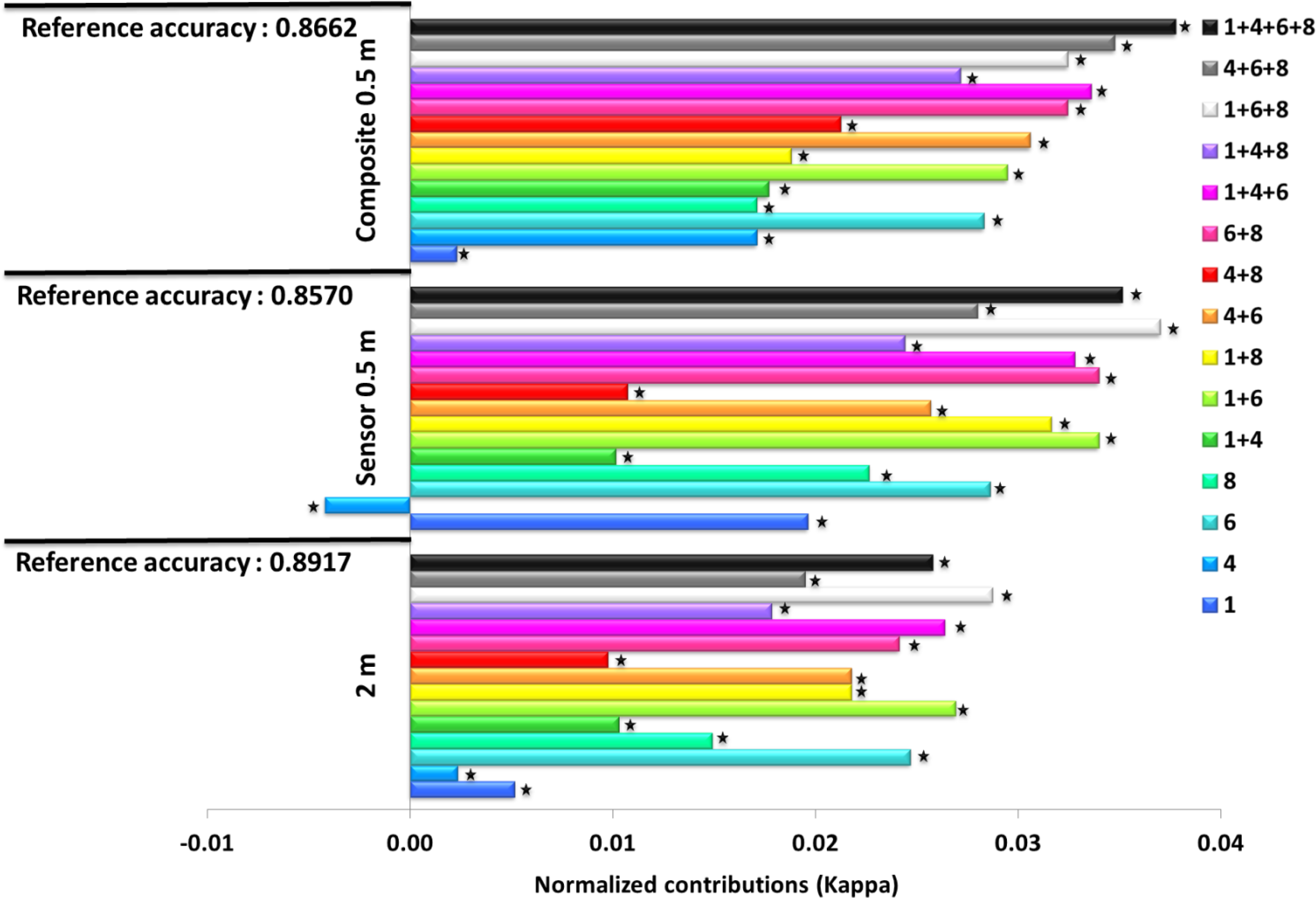
From the single band to the four band combination, the normalized contributions of the 15 combinations, built only with novel WV2 bands (coastal, yellow, NIR1 and NIR2) systematically increased the appa coefficient (κ) of the commonly used four band classification (Figure 4). The overall best single and combined contributions were attributed to the red edge band (κgain = 0.0247) and to the coastal-red edge-NIR2 combination (κgain = 0.0287) (cf. 
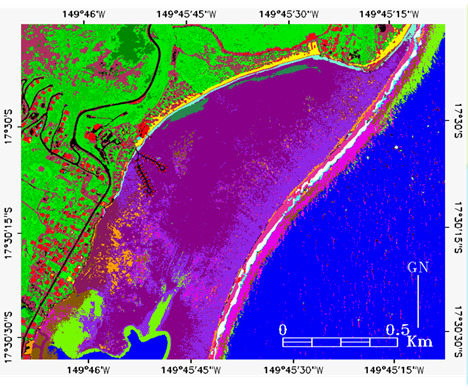
Figure A2 in Appendix for the classification map). Adding the red edge band enabled the spectral gap occurring between the red and NIR1 bands to be bridged, enhancing the discrimination among classes that show identifiable reflectance/absorbance within this spectral range. Note that the red edge penetration into water is expected to reach 0.7 m [33]. This assumption was confirmed by the best PA/UA results, indicating that: (1) the fleshy and encrusting algae received the highest contribution (UAgain = 18.18%) from all combinations, including either the red edge or the NIR2 bands, (2) the hard coral thicket was strongly enhanced by the coastal-red edge-NIR2 and four band combination (PAgain = 16.95%), (3) the tar was reinforced by all combinations, including either the red edge or the NIR2 bands (PAgain = 11.11%), and (4) the emergent vegetation benefited from the red edge and coastal-red edge combinations (UAgain = 10.59%) (Table 2). Regarding the emergent vegetation and the fleshy and encrusting algae (composed of Turbinaria spp. and encrusting algae), the importance of the integration of the red edge might be correlated with the detection of high reflectance inherent to chlorophyll organisms, also called the red-shift effect. Conversely, the red edge, sometimes called the far red, was demonstrated to correspond to the absorbance of photosystem I, while photosystem II was driven by the red wavelengths [34]. Stretching out the QB2 spectral windows, both coastal and NIR2 favored a better distinction among coastal classes. The contribution of coastal band to emergent vegetation and hard coral thicket might be related to the detection of the first peak of chlorophyll-a [28], hitherto undetectable for the traditional blue-bottomed sensor. Detecting beyond 1,000 nm (more than 150 nm over the QB2 upper boundary), NIR2, strongly absorbed by water, enabled the misclassifications occurring between land and water classes to be avoided. Of special relevance was the combined effect of the three and four band series, pointing out that a classification of hard coral thicket could be successful with a 400–1,000 nm spectrum range, despite the coarse spectral resolution (eight band average: 56 nm).
The most negative PA and UA contributions involved the yellow-NIR2 combination and were related to the hard coral/algae patches (losses: −20.88% and −18.38%, respectively) (Table 2). The misclassification associated with the yellow band might be the consequence of the subtle spatial heterogeneity of water composition occurring along the coast, due to terrestrial run-off. Matching the reflectance peak of surface waters containing CDOM [17], the yellow band might lead to misclassifications over the coastline-contiguous classes, such as the hard coral/algae patches. The overall accuracy supported this assessment, since the yellow band was the lowest contributor (0.0024), and its presence within the four band combination (coastal-yellow-red edge-NIR2) impaired the intuitively-expected best contribution. Following the advances tied to hyperspectral measurements, the WV2 yellow band coupled with in situ measurements should be further investigated regarding information from the water column, so that the inherent optical properties (IOP) could be better modelled across regional areas.

3.2. Patterning Classification Accuracy with Spatial Enhancement

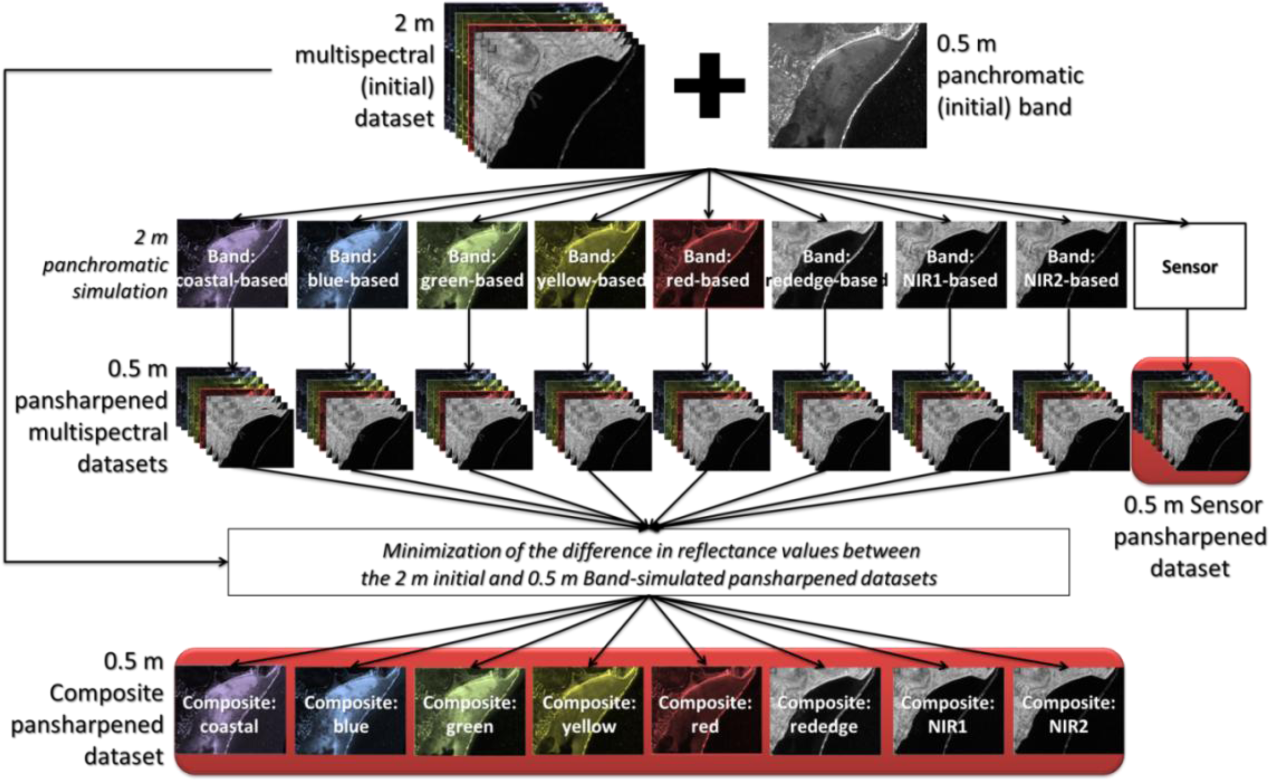
The influence of the simulation method (cf. step 1 of the Pan-sharpening procedure, Section 2.4, and 
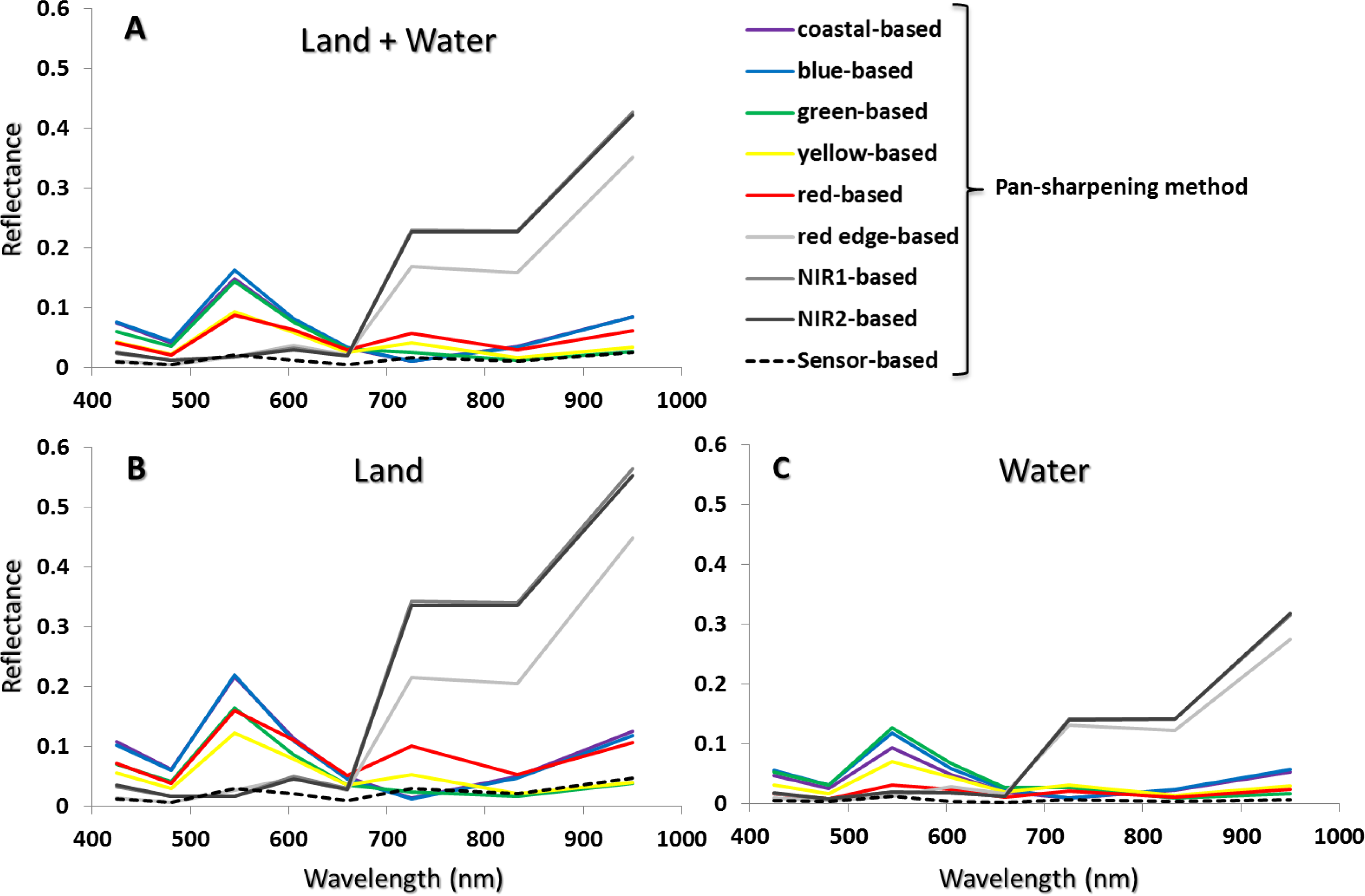
Figure 2) on the spectral properties of at-surface reflectance was assessed by computing the absolute average difference of the training pixels per band issued from the initial (2 m) and nine Pan-sharpened MS imageries (Figure 5). The difference was first computed based on the seamless study area, spanning the 21 ground-truth regions of interest, keeping the integrity of the reefscape irrespective of the coastline boundary (Figure 5A). Splitting the study area into nine land and 12 water areas, two differences were calculated in order to account for the land- and water-related specificity of spectral responses (Figure 5B,C). Overall, the sensor simulation displayed the lowest differences, irrespective of the level of the coast integrity, outperforming most of the eight band simulations. However, the sensor simulation was locally (at the wavelength scale) surpassed by some band simulations (e.g., red edge-based band simulation at 545 nm and coastal-based band simulation at 725 nm in the land + water analysis). Some spectral patterns related to band simulations emerged from the seamless and splitting analyses. While the NIR-based band simulations minimized the differences in the visible spectrum, the visible-based band simulations minimized the difference in the NIR spectrum. Conversely, the NIR- and visible-based band simulations maximized the differences in the NIR and visible spectral ranges, respectively (Figure 5).
Based on observations of the eight band simulations (excluding the sensor simulation, cf. Figure 5), a Pan-sharpened composite MS imagery was built from the band-based simulation displaying the smallest difference for each spectral band (Table 3). The resulting Pan-sharpened composite dataset thereafter provided a very high spatial resolution dataset, whilst minimizing the spectral deviation from the initially collected pixel values.
The effect of the enhancement of spatial scale on overall classification was examined as a function of the two simulation techniques employed in the Pan-sharpening procedure. The refinement of the spatial scale tended to slightly diminish the overall consistency between trained and validated pixels attendant with the measured 2 m standard four band dataset (Figure 4). Nevertheless, the proposed composite Pan-sharpening technique (κloss = −0.0255) was less impacted by the traditional sensor technique (κloss = −0.0347). The sensor modality showed the same categorical boundaries as those of the overall 2 m performance, i.e., highest and lowest contributions driven by the coastal-red edge-NIR2 (κgain = 0.037) and the yellow series, which was negative (κloss = −0.004). The composite modality was delimited by the coastal and four band series (κgain = 0.0023 and 0.0378, respectively). A pattern emerged from this latter modality, clearly separating the lowest contributions with no red edge and the highest contributions, including the red edge band.
According to previous results, we could hypothesize that the gap bridging, provided by the red edge integration into WV2 bands, was better exploited by the composite than the sensor simulation. On the other hand, the spectral deviation of the red edge signatures between the 2 m and the composite 0.5 m datasets was minimized by the coastal band, outperforming the 0.5 m sensor-driven deviation (Table 3). This result pointed out the existing complementarities of the red edge and the coastal information, which substantially improved the signals traditionally carried by the NIR-green couple (Table 3). Our composite simulation might also confer better results, because of accounting for the coastal band (400–450 nm), which was excluded from the sensor simulation (the WV2 Pan band spectrally starting at 450 nm). When dealing with Pan-sharpened-driven overall classification, we strongly advocate to use this proposed simulation technique in order to differentiate better among land and water classes with the integrated quasi-continuous optical spectrum.
The component substitution method, employed in this study, was based on a spectral combination of eight bands, without any spatial filtering of the Pan band. Advances in Pan-sharpening have been considerably motivated by the use of the multiresolution analysis. The principle is to decompose the imagery at various spatial resolutions, so that the details of the Pan image can be injected into the original MS dataset. The most successful decomposition functions are the generalized Laplacian pyramid and redundant shift-invariant wavelet and contourlet filtering of the Pan band [35].
The fusion products derived from the sensor and composite techniques were empirically assessed as spectral difference with the original dataset. Some protocols exist for evaluating the quality of fused images, such as the Khan’s protocol, which integrates the properties of other protocols in order to define spectral and spatial quality indices at full scale [35]. In the near future, the composite technique will be assessed with those recent progresses in quality measures in order to compare its efficiency with other techniques.
At the patch level, scaling up the spatial resolution led to an overall rise of spectral contributions (Tables 4 and 5). The sensor technique (Table 4) displayed the highest contributions in both land and water classes, namely the hard coral thicket (PAgain = 30.36% with coastal-red edge-NIR2), tar (UAgain = 18.94% with NIR2, coastal-NIR2, coastal-yellow-NIR2 and coastal-red edge-NIR2 series), hard coral bommie (UAgain = 17.81% with the four band combination) and emergent vegetation (PAgain = 16.67% with red edge and red edge-NIR2). The lowest contribution was attributed to the composite modality, involving the yellow band, which contributed in decreasing the UA hard coral thicket by −9.29%. However, the sensor simulation (Table 5) produced the three remaining lowest contributions, namely emergent vegetation (UAloss = −8.73% with the yellow-NIR2 combination), reef matrix (PAloss = −7.89% with yellow-red edge and yellow-red edge-NIR2 associations) and mature vegetation (PAloss = −7.04% with coastal-yellow and coastal-yellow-NIR2 combinations). While the average maximum PA and UA increased with spatial refinement, the range computed between average maximum and minimum PA and UA increased and decreased for land and water classes, respectively (Table 6). Those findings underlined two gradients of the accuracy stability: one for land classes ranging from high to low resolution; the other one for water classes ranging from low to high resolution. Following the pattern deciphered in the 2 m results, the red edge, associated or not with NIR2, was of profit for the emergent vegetation and considerably beneficial when combined with coastal, NIR2 and even yellow for both hard coral classes (Tables 4 and 5). These results could be explained by the same arguments mentioned in Section 3.1, namely spectral continuity, offered by the gap fulfilled by the red edge, detecting the reflectance/absorbance of chlorophylls, and yellow, as well as the spectral extension of the gamut with coastal and NIR2, sensing the first peak of chlorophyll-a and water, respectively. However, singly considered, the yellow band created discrepancies over hard coral thicket (UAloss = −9.29%), as well as hard coral/algae patches (UAloss = −6.72%). The yellow-driven counter performance might be due to the suspended sediment in the water column, since hard coral/algae patches attested to it (cf. explanation in Section 3.1), but also to the method itself, since the spectral difference between the 2 m and composite 0.5 m was the highest (Table 3). When dealing with Pan-sharpened images at the patch level, it is recommended to adopt the sensor approach to improve the classification accuracies of both land and water classes.

3.3. Classification Accuracy According to the Coast Integrity

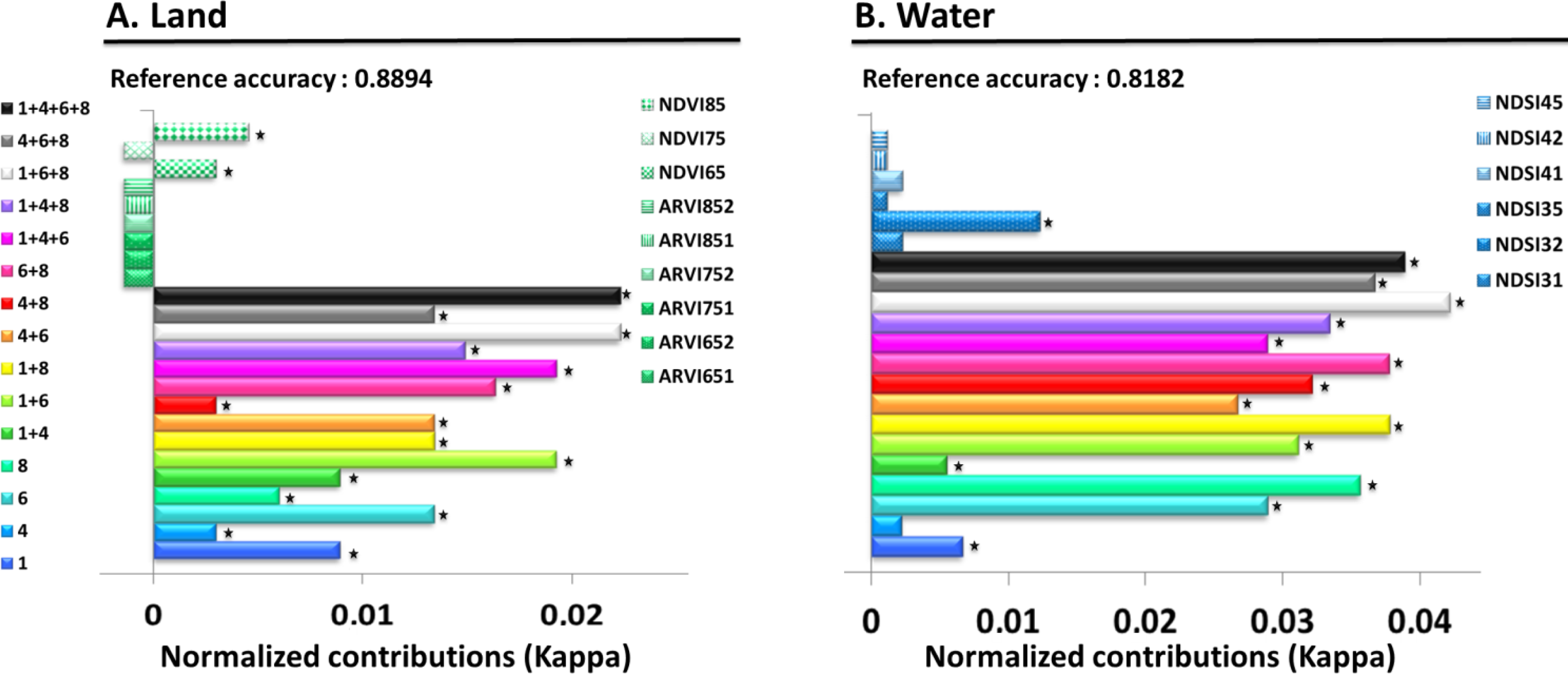
The splitting of the original 2 m coast into its land and water bodies differentially altered their respective overall classification accuracy (Figure 6). While the kappa coefficient related to land barely reduced to 0.8894 (κloss = −0.0023), for water, it decreased to 0.8182 (κloss = −0.0735). Considering only the land, the lowest spectral contribution was attributed to the yellow band (κgain = 0.0029), and the most gaining series involved coastal-red edge-NIR2 and a four band combination (κgain = 0.0223). Concerning vegetation indices, all ARVI and red-NIR1 NDVI brought negative contributions, while red-red edge NDVI and red-NIR2 NDVI supported slight contributions (topping at 0.0045 for the latter index). As for water partition, the yellow band brought the least important contribution (κgain = 0.0022), and the prime combination was based on the coastal-red edge-NIR2 association (κgain = 0.0422). All hard coral-related NDR furnished valuable information, increasing by 0.0011 (green-red, yellow-blue, yellow-red), 0.0022 (green-coastal, yellow-coastal) and 0.012 (green-blue). Regarding the land classes, the yellow band might be the least important contributor, since its spectral sensitivity does not correspond to any primary reflectance peaks of the vegetation pigments (cf. [36]). Although the yellow band provided the smallest contribution to both realms, it seemed that it was more prejudicial to the water class, given the best contribution was deprived of the yellow band. Once again, the spectral matching of the reflectance peak of CDOM-borne waters and the yellow band might entail inconsistencies over water classes somewhat masked by suspended matter in the water column. Arguing in favour of the increased power of discrimination with the quasi-continuity of the spectrum, the three and four band combination furnished the best results. The contribution of the land band ratios might be associated with the well-recognized spectral behaviour of the chlorophyll vegetation: strong absorption and reflection in the red and NIR wavelengths, respectively. Even if the traditional red wavelengths got involved in both ratios, the two related NIR wavelengths belonged to the novel WV2 spectral capabilities, the red edge band, bridging the traditional QB2 red and NIR1 bands, and the NIR2 band, considerably stretching out the NIR1 band to longer wavelengths. These findings unequivocally underscored the better proficiency of red edge and NIR2 bands for detecting vegetation reflectance compared to the commonly used NIR1 band, as found by [37]. Even though ARVI was better recognized to reduce the atmosphere effects than the NDVI index [38], it only worsened the classification accuracy of land classes. However, this counter-performance might be attributed to the fixing of the γ value at one. Provided with a γ value equalling 0.7, the ARVI index, applied to atmospherically uncorrected data, was demonstrated to be most capable of decreasing the atmospheric influence [38]. We therefore suggest that various γ values should be tested in further vegetated land classifications.
At the patch scale, the integrative approach of the coast turned out to be more prejudicial to land patch classes and more profitable to water patch classes, regardless of the PA and UA (Table 6). When singly considered, the land patch classes only benefited from the best contributions of 9.72% for UA emergent vegetation (with red edge band), of 8.89% for PA grass (with red edge, coastal-red edge, red edge-NIR2 and coastal-red edge-NIR2 combinations) and showed the least efficient contributions of −2.3% for PA bare soil (with yellow-NIR2, red edge-NIR2 and yellow-red edge-NIR2) and of −2.36% for UA roof (with yellow-NIR2) (Table 7). While the best contributions stemming from vegetation indices reached 3.85% for PA emergent vegetation (with red-NIR2 NDVI), the worst contribution was attributed to this same index with PA bare soil (i.e., PAloss = −2.3%). The grass and emergent vegetation classification accuracies were successively improved by the red edge band and red-NIR2 NDVI. As previously mentioned, the value of the red edge band might be strongly associated with the detection of reflectance/absorbance peaks of chlorophylls-a and -b and the utilization of NIR2, contiguous to the short-wavelength IR (SWIR). The resulting NDVI might optimize the detection of chlorophyll reflectance in avoiding the detection in the very NIR of vegetation absorbance attendant with its phenology and/or vigor [39].
On the other hand, singly considered, the water patch classes received a considerably prime contribution of 40% for PA hard coral bommie (with the coastal-NIR2 combination), 30% for UA hard coral bommie (with red edge-NIR2 and coastal-red edge combinations) and the poorest contributions of only −3.85% for UA hard coral/algae patches (coastal-yellow-NIR2) and of −1.18% for PA reef matrix (with the yellow band) (Table 7). Linked with the coastal, red edge and NIR2 bands, the strong enhancement of hard coral bommie might be explained by the detection of the first peak of chlorophyll-a, red-shift effect and, lastly, SWIR or the refinement of the land-water discrimination. The UA hard coral bommie benefited from green-coastal hard coral-related index (UAgain = 11.06%), while the PA reef matrix was lowered (PAgain = 4.71%) with the green-red, yellow-blue and yellow-red hard coral indices. The green-coastal NDR result firmly concurred with the finding of [28], demonstrating that it was likely to be a robust proxy for detecting coral pigments. Since this band ratio is required to be sensitive to pigments showing a high reflectance in the coastal band and a low reflectance in green coastal, the peridinin might turn out to be a good candidate. The difference existing between average maximum and minimum PA and UA was obviously lower for both land and water classes when the coast was examined according to a dichotomous approach (Table 6). This result indicated a higher stability in accuracies of the cut-off than the integrative scene, which might be due to the spectral and contextual specificity of the terrestrial and aquatic classes.
The increased contributions of the spectral combinations could be the consequence of the dramatic diminution of the overall classification accuracy. It is noteworthy that the overall classification accuracy of the integrated scene was greater than that of the fragmented coast. This result might reveal the “emergent properties that arose from spatial coupling of spectrally-derived local ecosystems” [40]. This citation, referred to as the concept of meta-ecosystem, could be defined as a “set of ecosystems connected by spatial flows of energy, materials and organisms across ecosystem boundaries” [40]. The bespoke coast-ecosystem could adequately match such a concept that will target ecological issues, commonly restrained to land and marine realms exclusively, in considering tropical watershed and nearshore ecosystems as spatially interconnected nodes of ecological processes across different spatial scales. Fluxes of materials and organisms occurring at the watershed/nearshore interface could, thereby, be looked at using a powerful theoretical framework. Monitoring the spatial assemblage of vegetation productivity and diversity (using red edge-NIR2 NDVI) with sedimentation (using yellow band) will not only enable the bilateral relationships to be quantitatively assessed, but also provide the potential to study the reciprocal influences that the hard coral/algae patches and the emergent/mature vegetation exert on each other’s functioning (coastal protection and sedimentation, respectively). Merging the coast-ecosystem concept with the WV2-based spatial patterning will furnish a timely method to analyze the structure and dynamics of coral-related meta-ecosystems at various scales and model the influence of watershed management on reef maintenance of the ecological services.

4. Conclusions

The tropical coastal zone ranging from the vegetated volcanic ridge to the outer reef through urbanized coastal fringe (nine terrestrial + 12 marine classes) has been successfully classified using the standard four band combination (blue: 2, green: 3, red: 5, NIR1: 7) and the support vector machine algorithm (kappa = 0.8917). Built only with the novel WorldView-2 bands (coastal: 1, yellow: 4, red edge: 6, NIR2: 8), the 15 combinations systematically increased the overall classification accuracy of the standard classification. The overall best single and combined contributions were attributed to the red edge band (κgain = 0.0247) and coastal-red edge-NIR2 combination (κgain = 0.0287), providing a significant increase of tar (Producer’s Accuracygain = 11.11%) and fleshy and encrusting algae (User’s Accuracygain = 18.18%) classes, respectively. On the other hand, while the addition of the yellow-NIR2 combination to the standard four bands brought an overall positive contribution, it dramatically impacted the hard coral/algae patches class (PAloss = −20.88%).
Enhancement of spatial resolution declined the standard classification accuracy, depending on the Pan-sharpening technique at stake. Our proposed composite method, selecting the WorldView-2 band minimizing the difference with initial data values per band (κ = 0.8662), provided better overall results than the commonly used sensor method, based on the spectral sensitivity of the inherent bands (κ = 0.857). However, the sensor technique produced the highest contributions with coastal-red edge-NIR2 combination akin to the tar (UAgain = 18.94%) and hard coral thicket (PAgain = 30.36%) classes. Partitioning the coast into its terrestrial (κ = 0.8894) and aquatic (κ = 0.8182) components lowered the standard classification accuracy. While the land-related emergent vegetation class mostly benefited from the red edge band (UAgain = 9.72%) and red-NIR2 NDVI (PAgain = 3.85%), the water-related hard coral bommie class was highly enhanced by the coastal-NIR2 combination (UAgain = 40%) and green-coastal NDR (UAgain = 11.06%).
The contributions of the added WorldView-2 bands to patch classification accuracy were inversely correlated with the overall classification accuracy. We discussed the spectral, methodological and ecological properties that have the potential to explain those novel findings. By enhancing the spectral discrimination at the individual massive plant and coral level (0.5–2 m), VHR spaceborne remote sensing is able to provide innovative insights into the evolution of tropical coastal ecosystems from local to regional scales, to predict the influence of anthropogenic and climate changes and to help design optimized management and conservation frameworks.

Acknowledgments

The first author gratefully acknowledges the technical staff from CRIOBE for validation sampling and the French Agency of Marine Protected Areas for the acquisition of the WorldView-2 imagery. The authors are also indebted to Manuscriptedit.com and Matthieu Huot for the sound English correction and to the reviewers for their relevant comments and suggestions.

Conflict of Interest

The authors declare no conflict of interest.

References

  1. Levin, L.A.; Boesch, D.F.; Covich, A.; Dahm, C.N.; Erseus, C.; Ewel, K.C.; Kneib, R.T.; Moldenke, A.; Palmer, M.A.; Snelgrove, P.; et al. The function of marine critical transition zones and the importance of sediment biodiversity. Ecosystems 2001, 4, 430–445. [Google Scholar]
  2. Costanza, R.; d’Arge, R.; de Groot, R.; Farber, S.; Grasso, M.; Hannon, B.; Limburg, K.; Naeem, S.; O’Neill, R.; Paruelo, J.; et al. The value of the world’s ecosystem services and natural capital. Nature 1997, 387, 253–260. [Google Scholar]
  3. Bellwood, D.R.; Hughes, T.P.; Folke, C.; Nyström, M. Confronting the coral reef crisis. Nature 2004, 429, 827–833. [Google Scholar]
  4. McGinley, M.; McClary, M. Threats to Coral Reefs. In Encyclopedia of Earth; Cleveland, C.J., Ed.; Environmental Information Coalition, National Council for Science and the Environment: Washington, DC, USA, 2008. [Google Scholar]
  5. Wolanski, E.; Richmond, R.; McCook, L.; Sweatman, H. Mud, marine snow and coral reefs: The survival of coral reefs requires integrated watershed-based management acticities and marine conservation. Amer. Sci 2003, 91, 44–51. [Google Scholar]
  6. Richmond, R.H.; Rongo, T.; Golbuu, Y.; Victor, S.; Idechong, N.; Davis, G.; Kostka, W.; Neth, L.; Hamnett, M.; Wolanski, E. Watersheds and coral reefs: Conservation science, policy and implementation. BioScience 2007, 57, 598–607. [Google Scholar]
  7. Mayer, L.; Barbor, K.; Boudreau, P.; Chance, T.; Fletcher, C.; Greening, H.; Li, R.; Mason, C.; Metcalf, K.; Snow-Cotter, S.; et al. A Geospatial Framework for the Coastal Zone: National Needs for Coastal Mapping and Charting; National Academies Press: Washington, DC, USA, 2004; p. 149. [Google Scholar]
  8. Bartier, P.M.; Sloan, N.A. Reconciling maps with charts towards harmonizing coastal zone base mapping: A case study from british columbia. J. Coast. Res 2007, 231, 75–87. [Google Scholar]
  9. Guenther, G.C.; Brooks, M.W.; LaRocque, P.E. New capabilities of the “SHOALS” airborne lidar bathymeter. Remote Sens. Environ 2000, 73, 247–255. [Google Scholar]
  10. Collin, A.; Long, B.; Archambault, P. Merging land-marine realms: Spatial patterns of seamless coastal habitats using a multispectral LiDAR. Remote Sens. Environ 2012, 123, 390–399. [Google Scholar]
  11. Green, E.P.; Mumby, P.J.; Edwards, A.J.; Clark, C.D. Remote Sensing Handbook for Tropical Coastal Management; Edwards, A.J., Ed.; UNESCO: Paris, France, 2000. [Google Scholar]
  12. Mishra, D.; Narumalani, S.; Rundquist, D.; Lawson, M. Benthic habitat mapping in tropical marine environments using Quickbird multispectral data. Photogramm. Eng. Remote Sensing 2006, 72, 1037–1048. [Google Scholar]
  13. Viedma, O.; Torres, I.; Pérez, B.; Moreno, J.M. Modeling plant species richness using reflectance and texture data derived from QuickBird in a recently burned area of Central Spain. Remote Sens. Environ 2012, 119, 208–221. [Google Scholar]
  14. Benet, A. Évolution des Zones Côtières en Milieu Insulaire et Impact du Changement Global: Perspectives 2100, Ph.D. Thesis, University of French Polynesia, Papeete, French Polynesia, 29 November 2010. 245.
  15. Pouteau, R.; Stoll, B. Fusion for Classes in Difficulty for Accurate and Speed Tropical Rainforests Classification. Proceedings of the IEEE International Geoscience and Remote Sensing Symposium, Vancouver, BC, Canada, 24–29 July 2011; pp. 740–743.
  16. Bricaud, A.; Morel, A.; Prieur, L. Absorption by dissolved organic matter of the sea (yellow substance) in the UV and visible domains. Limnol. Oceanogr 1981, 26, 43–53. [Google Scholar]
  17. Chen, S.; Chen, W.; Li, D. Remote Sensing of CDOM in Tidal Reach of Pearl River Estuary, China. Proceedings of The 2nd Academic Forum of Quantitative Remote Sensing of China, Beijing, China, 4–6 March 2011.
  18. Collin, A.; Hench, J.L. Towards deeper measurements of tropical reefscape structure using the WorldView-2 spaceborne sensor. Remote Sens 2012, 4, 1–23. [Google Scholar]
  19. Collin, A.; Planes, S. Enhancing coral health detection using spectral diversity indices from WorldView-2 imagery and machine learners. Remote Sens 2012, 4, 3244–3264. [Google Scholar]
  20. Mumby, P.J.; Clark, C.D.; Green, E.P.; Edwards, A.J. Benefits of water column correction and contextual editing for mapping coral reefs. Int. J. Remote Sens 1998, 19, 203–210. [Google Scholar]
  21. Purkis, S.J.; Pasterkamp, R. Integrating in situ reef-top reflectance spectra with Landsat TM imagery to aid shallow-tropical benthic habitat mapping. Coral Reefs 2004, 23, 5–20. [Google Scholar]
  22. Andrefouet, S.; Kramer, P.; Torres-Pulliza, D.; Joyce, K.E.; Hochberg, E.J.; Garza-Perez, R.; Mumby, P.J.; Riegl, B.; Yamano, H.; White, W.H.; et al. Multi-sites evaluation of IKONOS data for classification of tropical coral reef environments. Remote Sens. Environ 2003, 88, 128–143. [Google Scholar]
  23. Dalleau, M.; Andréfouët, S.; Wabnitz, C.C.; Payri, C.; Wantiez, L.; Pichon, M.; Friedman, K.; Vigliola, L.; Benzoni, F. Use of habitats as surrogates of biodiversity for efficient coral reef conservation planning in Pacific Ocean islands. Conserv. Biol 2010, 24, 541–552. [Google Scholar]
  24. Laben, C.A.; Brower, B.V. Process for Enhancing the Spatial Resolution of Multispectral Imagery Using Pan-Sharpening. US Patent 6,011,875, 4 January 2000.
  25. Amro, I.; Mateos, J.; Vega, M.; Molina, R.; Katsaggelos, A.K. A survey of classical methods and new trends in pansharpening of multispectral images. EURASIP J. Adv. Signal Process 2011, 79, 1–22. [Google Scholar]
  26. Tucker, C. Red and photographic infrared linear combinations for monitoring vegetation. Remote Sens. Environ 1979, 8, 127–150. [Google Scholar]
  27. Kaufman, Y.J.; Tanre, D. Atmospherically resistant vegetation index (ARVI) for EOS-MODIS. IEEE Trans. Geosci. Remote Sens 1992, 30, 261–270. [Google Scholar]
  28. Collin, A.; Hench, J.L.; Planes, S. A Novel Spaceborne Proxy for Mapping Coral Colonies. Proceedings of the International Coral Reef Symposium (ICRS), Cairns, Queensland, Australia, 9–13 July 2012.
  29. Pouteau, R.; Collin, A. Spatial location and ecological content of support vectors in an SVM classification of tropical vegetation. Remote Sens. Lett 2013, 4, 686–695. [Google Scholar]
  30. Vapnik, V.; Chervonenkis, A. Statistical Learning Theory. In Support Vector Machines for Pattern Recognition; John Wiley & Sons: New York, NY, USA, 1998. [Google Scholar]
  31. Foody, G.M.; Mathur, A. The use of small training sets containing mixed pixels for accurate hard image classification: Training on mixed spectral responses for classification by a SVM. Remote Sens. Environ 2006, 103, 179–189. [Google Scholar]
  32. Congalton, R.; Green, K. Basic Analysis Techniques. In Assessing the Accuracy of Remotely Sensed Data: Principles and Practices; Congalton, R., Green, K., Eds.; CRC Press: Boca Raton, FL, USA, 1999; Chapter 5. [Google Scholar]
  33. Smith, R.C.; Baker, K.S. Optical properties of the clearest natural waters (200–800 nm). Appl. Opt 1981, 20, 177–184. [Google Scholar]
  34. Koning, R.E. Light. Plant Physiology Information Website. 1994. Available online: http://plantphys.info/plant-phisiology/light.shtml (accessed on 22 March 2012).
  35. Aiazzi, B.; Alparone, L.; Baronti, S.; Garzelli, A. Quality assessment of pansharpening methods and products. IEEE Gesosci. Remote Sens. Newsl 2011, 161, 10–18. [Google Scholar]
  36. Gross, J. Pigments in Vegetables: Chlorophylls and Carotenoids; Van Nostrand Reinhold: New York, NY, USA, 1991; p. 351. [Google Scholar]
  37. Collin, A.; Planes, S. What is the Value Added of 4 Bands within the Submetric Remote Sensing of Tropical Coastscape? QuickBird-2 vs. WorldView-2. Proceedings of the IEEE International Geoscience and Remote Sensing Symposium, Vancouver, BC, Canada, 24–29 July 2011; pp. 2165–2168.
  38. Liu, G.R.; Liang, C.K.; Kuo, T.H.; Lin, T.H.; Huang, S.J. Comparison of the NDVI, ARVI and AFRI vegetation index, along with their relations with the AOD using SPOT 4 Vegetation data. J. Terr. Atmos. Ocean. Sci 2004, 15, 15–31. [Google Scholar]
  39. Kariyeva, J.; van Leeuwen, W.J.D. Environmental drivers of NDVI-Based vegetation phenology in central Asia. Remote Sens 2011, 3, 203–246. [Google Scholar]
  40. Loreau, M.; Mouquet, N.; Holt, R.D. Meta-ecosystems: A theoretical framework for a spatial ecosystem ecology. Ecol. Lett 2003, 6, 673–679. [Google Scholar]

Appendix

Figure A1. Comparisons of true color composite images (RGB: 532) of the (A) atmospherically-uncorrected (i.e., at-sensor radiance) and the (B) atmospherically-corrected (i.e., at-surface radiance) scenes.NB: Yellow and red stars symbolize land and water patch class sites (90 stations each except for Pool class, which has 75), respectively. Blue stars represent locations of the 36 ground control points. Black-contoured white arrows show the sites of the two zoom-ins.
Remotesensing 05 03583f7
Figure A2. Support Vector Machine-driven classification of 21 coastal patch classes derived from the standard spectral dataset (blue, green, red, and NIR1) enhanced by the three band combination (Coastal-red edge-NIR2): κ = 0.9173 (+0.0256).
Remotesensing 05 03583f8
Figure 1. Location of the study area in (A) Moorea, society island archipelago, (B) French Polynesia and (C) the true color composite image (RGB:532) of the study area.
Remotesensing 05 03583f1
Figure 2. Heuristic framework showing the composite and sensor Pan-sharpened multispectral (MS) datasets for identifying optimized Pan-sharpening methods with regard to the Pan simulation.
Remotesensing 05 03583f2
Figure 3. Study design aiming at assessing the contribution of the 15 spectral combinations, the nine vegetation indices and the six coral indices relative to the reference combination (IR:7, R:5, G:3, B:2) with respect to the ecological organization (land + water, land and water) and the spatial scale (2 m, composite 0.5 m and sensor 0.5 m).Nota bene (NB): 1 = Coastal, 2 = blue, 3 = green, 4 = yellow, 5 = red, 6 = red edge, 7 = NIR1, 8 = NIR2, NIR = near-infrared, NDVI = Normalized Difference Vegetation Index, ARVI: Atmosphere Resistant Vegetation Index, NDSI = Normalized Difference Scleractinian Index.
Remotesensing 05 03583f3
Figure 4. Bar plots of the overall normalized contributions of the 15 spectral combinations derived from the novel WV2 bands for the initial 2 m, the Pan-sharpened sensor 0.5 m, and the Pan-sharpened composite 0.5 m MS datasets.NB: 1 = Coastal, 4 = yellow, 6 = red edge, 8 = NIR2; Black stars indicate a significant difference between the distribution of correctly classified values related to the reference and combinations to-be-tested (Mann-Whitney U test, p < 0.01).
Remotesensing 05 03583f4
Figure 5. Segment plots of the absolute average difference of the reflectance values (per band) of the training pixels stemming from (1) the 2 m initial dataset and (2) eight band-based and one sensor-based 0.5 m Pan-sharpened datasets (i.e., nine various series) as a function of the coast integrity: (A) land + water; (B) only land; and (C) only water.
Remotesensing 05 03583f5
Figure 6. Bar plots of the land/water split overall normalized contributions of the 15 spectral combinations derived from new WV2 bands associated with (A) the nine vegetation indices for land classes and (B) the six coral indices for water classes.NB: 1 = Coastal, 2 = blue, 3 = green, 4 = yellow, 5 = red, 6 = red edge, 7 = NIR1, 8 = NIR2; Black stars indicate a significant difference between the distribution of correctly classified values related to the reference and to-be-tested combinations (Mann-Whitney U test, p < 0.01).
Remotesensing 05 03583f6
Table 1. Description of the 21 tropical coastal patch classes, comprising nine land classes showing anthropogenic features and 12 water classes.
Coastal ZonationPatch ClassDescription
RidgeRoofMetallic or vegetal covers of dwellings that can be white, red, green or brown colored
PoolSmall body of clear water localized nearby dwellings
GrassHerbaceous communities frequently mowed
ValleyMature vegetationArborescent (≥5 m) natural and cultivated species represented by Casuarina, Syzygium and Mangifera clumps and Cocos nucifera plantation
Emergent vegetationArbustive (≤5 m) natural and cultivated species represented by young tree stratum and facies of Miscanthus, Melinis, Psidium and Dodonea
Dry vegetationArborescent and arbustive species dominated by Leucaena
Coastal road networkTarPrimary transport axis characterized by asphalt-covered curve lines
Bare soilSecondary transport axis covered by reef pebbles and bare soil
BackshoreSandSupratidal coralligenous clastic sediment included in the 0.06–2 mm range
ForeshoreVery shallow sandIntertidal coralligenous clastic sediment included in the 0.06–2 mm range
NearshoreShallow sandSubtidal coralligenous clastic sediment included in the 0.06–2 mm range
Sandy pavementConsolidated coralligenous debris consisting of the nearshore platform
Hard coral/algae patches on sandy/muddy pavementConsolidated coralligenous debris sometimes showing scattered algae tufts and micro-atolls
Hard coral bommiePseudo-spherical massive colony dominated by Porites spp., S. rus and Montipora spp.
Hard coral thicketField of massive A. pulchra colony
AlgaeTufts or carpets of macroalgae dominated by Turbinaria spp., Padinae spp. and Sargassum spp.
Hard coral bommie on pavementSandy pavement over-mounted by patched massive coral colonies
Fleshy and encrusting algaeSeaward boundary of the lagoon covered by encrusting and Turbinaria spp. algae
FoamWhite body of water constituted by air-seawater mix
Reef matrixOceanic part of the reefs showing spurs-and-grooves reef forms
OffshoreOceanOptical deep water
Table 2. Class normalized contributions of the 15 spectral combinations derived from the novel WorldView-2 bands computed for (above sub-table) the producer’s accuracy and (below sub-table) the user’s accuracy.
RoofPoolGrassMature VegetationEmergent VegetationDry VegetationTarBare SoilSandVery Shallow SandShallow SandSandy PavementHard Coral/Algae Patches on Sandy/Muddy PavementHard Coral BommieHard Coral ThicketAlgalHard Coral Bommie on PavementFleshy and Encrusting AlgaeFoamReef MatrixOcean
1−0.01000.01000.010.07000.010−0.030.01−0.08000.0500.040
400.0400.0100.030.01−0.01000.020−0.01−0.030000.090.01−0.1−0.01
6−0.010.040.080.0400.020.11−0.01000.01000.10.15000.14−0.01−0.06−0.01
80.01000.0600.020.11−0.01000.01000−0.1000.1400.020
1+400.0200.0100.030.010.06000.010−0.0200.05000.090.01−0.040
1+6−0.0100.080.0300.020.110.05000.020−0.020.10.15000.140−0.050
1+80.010.0400.0500.020.110.06000.020−0.010.01−0.08000.1400.050
4+6−0.010.040.070.030.010.030.11−0.01000.010−0.010.070.140−0.010.140.01−0.09−0.01
4+800.020.070.01−0.010.030.11−0.01000.010−0.210.090.140−0.060.140−0.040
6+800.020.080.03−0.010.020.11−0.01000.01000.090.150−0.010.140−0.050
1+4+6−0.010.020.070.040.010.030.110.05000.010.01−0.020.070.15000.140−0.070
1+4+80.010.0400.0300.030.110.050000−0.020−0.02000.140.01−0.010
1+6+800.020.08000.020.110.03000.01000.120.17000.140−0.040
4+6+800.020.070−0.010.030.11−0.010000−0.020.060.140−0.010.140−0.050
1+4+6+800.020.0700.010.030.110.03000.010.01−0.020.070.17000.140−0.060
10.07−0.020000.030−0.020000.01−0.030.03−0.04000.0400.020
40.01000.0100.050.03000.0100.02−0.03−0.11−0.01−0.0100.050−0.010
60−0.020.010.010.110.050.05−0.0100.0100.01−0.080.050.05000.1800.130
80.01−0.0200.010.010.080.0500.01000.01−0.06−0.01−0.05000.18−0.010.050
1+40.06000.0100.040.04−0.0100.0100.01−0.03−0.030.03−0.0100.0500.010
1+60.05−0.020.0100.110.040.05−0.020000.02−0.050.060.04−0.0100.1800.110
1+80.06−0.0200.010.010.070.05−0.010.010.0100.03−0.080.01−0.01000.1800.060
4+60.0100.020.010.090.030.06−0.0100.0100.01−0.0700.04−0.0100.1800.090
4+80−0.020.0100.050.060.05−0.010.010.0100.01−0.180.060.02−0.01−0.110.1800.110
6+80−0.020.01−0.010.070.070.05−0.010.010.0100.01−0.080.080.04000.1800.120
1+4+60.05−0.020.020.020.090.040.06−0.0200.0100.01−0.050.020.04−0.010.010.1800.090
1+4+80.06000.010.010.050.05−0.010.010.0100.01−0.07−0.060−0.0100.1800.080
1+6+80.04−0.020.0100.070.050.05−0.020.010.0100.01−0.060.090.06−0.0100.1800.130
4+6+80−0.020.0100.050.050.05−0.010.010.0100−0.080.040.04−0.0100.1800.10
1+4+6+80.04−0.020.020.010.060.050.05−0.020.010.0100.01−0.070.030.04−0.010.010.1800.130
NB: the normalized contributions are color-coded according to a blue-red gradient (dark blue and red represent the most detrimental and beneficial contributions, respectively).
Table 3. Composition of the Pan-sharpened composite MS imagery with respect to coast integrity. Each selected Pan-sharpened band corresponds to the band of the eight band-based Pan-sharpening methods, minimizing the difference with initial data values for each spectral band.
CoastalBlueGreenYellowRedRed EdgeNIR1NIR2
Land + WaterRed edgeRed edgeRed edgeNIR2NIR2CoastalGreenGreen
LandRed edgeRed edgeNIR2NIR2Red edgeBlueGreenGreen
WaterRed edgeRed edgeRed edgeNIR2redCoastalGreenGreen
Table 4. Class normalized contributions of the 15 spectral combinations derived from the novel WV2 bands as a function of the sensor Pan-sharpening technique computed for (above sub-table) the producer’s accuracy and (below sub-table) the user’s accuracy.
RoofPoolGrassMature VegetationEmergent VegetationDry VegetationTarBare SoilSandVery Shallow SandShallow SandSandy PavementHard Coral/Algae Patches on Sandy/Muddy PavementHard Coral BommieHard Coral ThicketAlgalHard Coral Bommie on PavementFleshy and Encrusting AlgaeFoamReef MatrixOcean
1−0.010.020.100.06000.100000.010.030.140−0.02000.030.02
40−0.02−0.04−0.030000.0100000−0.02−0.020−0.010.050−0.050.01
6−0.02−0.020.13−0.030.1700.050.01000000.060.130−0.030.250−0.050.01
80.02−0.02−0.020.010.0200.070−0.010.01000.01−0.020.20−0.020.2500.030
1+40.010.020.05−0.070.03000.0900000.010.050.050−0.020.050−0.040.01
1+6−0.020.020.15−0.040.0800.050.10000−0.010.050.210−0.030.250−0.010.01
1+800.020.0500.0500.070.0700.0100−0.0100.230−0.030.2500.010.02
4+6−0.0200.13−0.040.1400.050.01000000.050.130−0.030.250−0.080.01
4+80.020−0.06−0.06000.05000.01000.01−0.020.070−0.030.250−0.040.01
6+80−0.020.1300.1700.050.01−0.010.0100−0.010.090.180−0.030.250−0.040.01
1+4+6−0.010.020.13−0.040.0900.050.10000−0.020.050.230−0.030.250−0.050.01
1+4+80.0100.02−0.070.0300.070.06−0.010.01000.010.030.180−0.030.250−0.010.01
1+6+800.020.12−0.040.1100.070.09−0.010.0100−0.020.080.30−0.030.250−0.050.01
4+6+8−0.0100.13−0.060.1400.050.01−0.010.010000.080.160−0.030.250−0.080.01
1+4+6+8000.16−0.040.1100.050.0500.0100−0.020.060.290.01−0.030.250−0.070.01
10.0700.060.010.1100.01−0.02000.01−0.01−0.040.050.120−0.02000.10
4−0.0100.01−0.02−0.05−0.010.0300.010.01−0.010−0.040.01−0.020.0100.020−0.040
6−0.0100.110.020.1400.18−0.010000−0.010.140.03−0.010.020.090−0.040
800−0.010.02−0.030.020.190.010.02000−0.010.090.0800.010.0900.040
1+40.0600.05−0.03000.05−0.010.010.020−0.01−0.060.050.040.01−0.02000.060
1+60.0700.1−0.040.120.010.18−0.02000.010−0.040.130.09−0.010.010.0900.050
1+80.0700.0400.050.020.19−0.020.0100.010−0.050.10.1−0.010.010.0900.090
4+6−0.0100.1100.1200.18−0.0100.0100−0.060.130.040.010.010.090−0.050
4+800−0.030.01−0.0900.1900.020.0100−0.040.020.020.010.010.090−0.010
6+8−0.0100.110.040.1400.19−0.010.0200000.130.11−0.010.010.090−0.040
1+4+60.0600.11−0.030.1100.18−0.020.010.010.010−0.070.130.070.01−0.010.0900.070
1+4+80.0500.03−0.03−0.020.010.19−0.010.0100.010−0.050.080.080.01−0.010.0900.10
1+6+80.0500.1−0.010.110.010.19−0.020.010.010.010−0.020.170.11−0.0100.0900.050
4+6+8−0.0100.110.010.11−0.010.19−0.020.010.0100−0.030.150.060.010.010.090−0.050
1+4+6+80.0400.11−0.020.1400.19−0.020.0100.010−0.040.180.080.01−0.010.0900.050
NB: the normalized contributions are color-coded according to a blue-red gradient (dark blue and red represent the most detrimental and beneficial contributions, respectively)
Table 5. Class normalized contributions of the 15 spectral combinations derived from the novel WV2 bands bands as a function of the composite Pan-sharpening technique computed for (above sub-table) the producer’s accuracy and (below sub-table) the producer’s accuracy and (below sub-table) the user’s accuracy.
RoofPoolGrassMature VegetationEmergent VegetationDry VegetationTarBare SoilSandVery shallow SandShallow SandSandy PavementHard Coral/Algae Patches on Sandy/Muddy PavementHard Coral BommieHard Coral ThicketAlgalHard Coral Bommie on PavementFleshy and Encrusting AlgaeFoamReef MatrixOcean
10.0100.0200000.040000−0.030.01−0.070000.010.030.01
40−0.020.050.01−0.010.010.07000.0100.010.05−0.04−0.0100.010.1300.1−0.01
60.0100.1300.010.010.10.0100.01000.020.070.030−0.030.1500.08−0.01
8−0.01−0.020.02000.010.1000.0100.010.02000−0.010.1500.060
1+4−0.01−0.020.050.02−0.040.010.060.0200.0100.010.05−0.030.010−0.020.110.010.10.01
1+6000.130.020.010.010.090.0400000.020.070.040−0.030.150.010.040.01
1+80.0100.01000.010.10.0200.01000.020.01−0.030−0.010.150.010.040.01
4+6000.130.0200.010.080.0100.01000.050.0700−0.020.1500.15−0.01
4+8−0.01−0.020.050.04−0.040.010.1000.01000.050.01−0.010−0.020.150.010.13−0.01
6+80.010.020.120.010.030.010.10.0100.01000.020.070.070−0.030.150.010.1−0.01
1+4+600.020.140.0200.010.080.0200.0100.010.050.0700−0.030.150.010.140.01
1+4+8000.050.04−0.010.010.110.0200.0100.010.05−0.01−0.01000.150.010.130.01
1+6+80.01−0.020.130.010.030.010.10.0200.01000.020.070.080−0.030.150.010.060.01
4+6+80.010.020.130.020.010.010.10.0100.01000.050.070.030−0.020.150.010.14−0.01
1+4+6+80.0100.140.020.010.010.110.0200.0100.010.050.070.040−0.030.150.010.140.01
10.040000.0200−0.020.02000−0.01−0.040.0300.01−0.010.01−0.050
4−0.020000.06−0.040.130000.01−0.010.12−0.04−0.090.0200.110.010.140
6000.020.010.15−0.050.150.020.020000.0200.010.02−0.010.110.010.110
8−0.010000.02−0.020.14−0.010.0200.0100.07−0.050.03−0.0200.1100.030
1+40.020−0.0200.05−0.030.12−0.02000.01−0.010.08−0.04−0.060.02−0.010.110.010.150
1+60.0400.020.010.15−0.030.1400.02000−0.020.010.05000.110.010.090
1+80.020000.01−0.020.1400.02000.010.05−0.050.05−0.020.010.110.010.010
4+6000.0200.16−0.040.150.020.01−0.010.01−0.010.09−0.030.010.0200.110.010.120
4+8−0.010−0.020.010.05−0.020.1500.01−0.010.01−0.010.15−0.04−0.030.02−0.010.110.010.070
6+80.0200.010.020.12−0.020.140.010.020000.070.010.050.01−0.010.110.010.070
1+4+60.0400.0200.16−0.030.150.010.0100.01−0.010.08−0.0100.0200.110.010.110
1+4+80.02000.010.06−0.020.150.010.0100.0100.17−0.06−0.020.0200.110.010.080
1+6+80.0200.020.020.14−0.020.1400.020000.030.040.06000.110.010.080
4+6+80.0200.020.010.16−0.040.150.010.02−0.010.0100.140.010.010.02−0.010.110.010.080
1+4+6+80.0300.020.010.16−0.030.150.010.0200.01−0.010.130.040.010.0200.110.010.090
NB: the normalized contributions are color-coded according to a blue-red gradient (dark blue and red represent the most detrimental and beneficial contributions, respectively).
Table 6. Range and maximum of the average contribution producer’s and user’s accuracies for land and water classes as a function of spatial resolution and coast integrity. PA, producer’s accuracy; UA, user’s accuracy.
LandWater

PAUAPAUA

RangeMaximumRangeMaximumRangeMaximumRangemaximum
Original 2 m4.944.684.223.988.244.327.754.05
Sensor 0.5 m8.136.078.376.37.3266.044.6
Composite 0.5 m5.034.395.644.45.954.67.234.9
Split 2 m3.552.843.753.065.285.265.895.39
Table 7. Land/water split class normalized contributions of the 15 spectral combinations derived from the (above sub-table) the nine vegetation indices for the land classes and (below sub-table) the six coral indices for the producer’s and the user’s accuracies.
RoofPoolGrassMature VegetationEmergent VegetationDry VegetationTarBare SoilSandRoofPoolGrassMature VegetationEmergent VegetationDry VegetationTarBare SoilSand
1−0.01000000.010.0700.06000−0.010.010−0.010
40.01−0.0200.010.0100.01−0.010−0.0200.01000.010.010.010
6−0.01−0.020.090.010.0300.01−0.010−0.0200.0300.10.01000
80.01−0.0200.05000.01−0.010−0.02000.0100.05−0.010.010.01
1+40−0.02000.0100.010.0600.0500.010−0.010.01000
1+6−0.01−0.020.090.010.01−0.010.010.0600.0400.02−0.010.10.010−0.010
1+80000.040−0.010.010.0700.0700−0.01−0.010.030−0.010.01
4+6−0.0100.080.010.0300.01−0.010−0.0100.0300.080.01000
4+80.01−0.0200.030.0100.01−0.020−0.0200.010−0.010.0300.010.01
6+8000.090.040.03−0.010.01−0.020−0.0200.03−0.010.080.04−0.0100.01
1+4+6−0.01−0.020.0800.0300.010.0600.0400.0300.070.010−0.010
1+4+80.01−0.0200.040.0100.010.0600.0500.010−0.010.04000.01
1+6+80−0.020.090.040.01−0.020.010.0600.0500.02−0.020.080.04−0.01−0.010.01
4+6+8000.080.040.01−0.010.01−0.020−0.0200.02−0.010.070.03000.01
1+4+6+80−0.020.080.030.0100.010.0600.0500.0200.070.030−0.010.01
ARVI65100−0.010.010.03−0.020−0.010−0.0100.01−0.0100000
ARVI65200−0.010.010.03−0.020−0.010−0.0100.01−0.0100000
ARVI75100−0.010.010.03−0.020−0.010−0.0100.01−0.0100000
ARVI75200−0.010.010.03−0.020−0.010−0.0100.01−0.0100000
ARVI85100−0.010.010.03−0.020−0.010−0.0100.01−0.0100000
ARVI85200−0.010.010.03−0.020−0.010−0.0100.01−0.0100000
NDVI650.010−0.010.010.04−0.02000000.02−0.010.0100.0100
NDVI7500−0.010.010.03−0.020−0.010−0.0100.01−0.0100000
NDVI850.01000.010.0400−0.020−0.0200.020.010.0200.0100
Table 7. Land/water split class normalized contributions of the 15 spectral combinations derived from the (above sub-table) the nine vegetation indices for the land classes and (below sub-table) the six coral indices for the producer’s and the user’s accuracies.
Very Shallow SandShallow SandSandy PavementHard Coral/Algae Patches on Sandy/Muddy PavementHard Coral BommieHard Coral ThicketAlgalHard coral Bommie on PavementFleshy and Encrusting AlgaeFoamReef MatrixOceanVery Shallow SandShallow SandSandy PavementHard Coral/Algae Patches on Sandy/Muddy PavementHard Coral BommieHard Coral ThicketAlgalHard Coral Bommie on PavementFleshy and Encrusting AlgaeFoamReef MatrixOcean
1000.0100.030.03000000.0100000.040.0200.01000.010
400.010.0100.020.010000−0.01−0.01000.01−0.010000.030000
600.010.0100.220.0900000.040.01000.010.010.180.1200.01000.05−0.01
80000.010.170.0900000.140.02000−0.040.380.0800.02000.040
1+400000.020.0100000.010.02000−0.010.040.040000−0.010
1+600.01000.250.0900000.040.02000.010.010.20.1300000.050
1+800−0.0100.170.1200000.160.02000−0.010.40.0900000.05−0.01
4+6000.0100.220.0900000.020.0100000.180.0900.03000.050
4+8000.0100.0600000.140.02000−0.030.40.0500.030000
6+8000.0100.30.0300000.130.02000−0.020.370.1200.030000
1+4+600000.230.0900000.040.0200000.20.1200.01000.050
1+4+800000.0900000.140.02000−0.040.40.0700.02000.020
1+6+8000.0100.30.0600000.140.02000−0.020.3700.02000.030
4+6+8000.0100.280.0300000.130.02000−0.030.370.1200.030000
1+4+6+8000.0100.270.0500000.140.02000−0.030.370.1200.03000.020
NDR3200.0100.010.020.030000−0.040000.010.0100.0100000.010
NDR3100.010.010.01−0.020.0100000.080.01000.010.020.110.020−0.0100−0.020
NDR3500.0100.010.020.030000−0.050000.010.01−0.010.0100000.010
NDR4200.0100.010.050.010000−0.050000.010.02−0.010.0100000.010
NDR4100.0100.010.020.010000−0.040000.010.01−0.01000000.010
NDR4500.0100.010.020.030000−0.050000.010.01−0.010.0100000.010
NB: The normalized contributions are color-coded according to a blue-red gradient (dark blue and red represent contributions, respectively).

