Landslide Displacement Monitoring Using 3D Range Flow on Airborne and Terrestrial LiDAR Data


Abstract
:1. Introduction
2. Related Work
3. Data and Methods
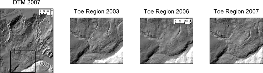
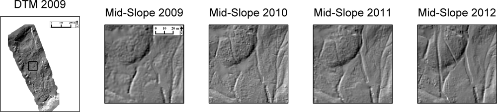
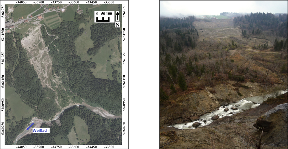
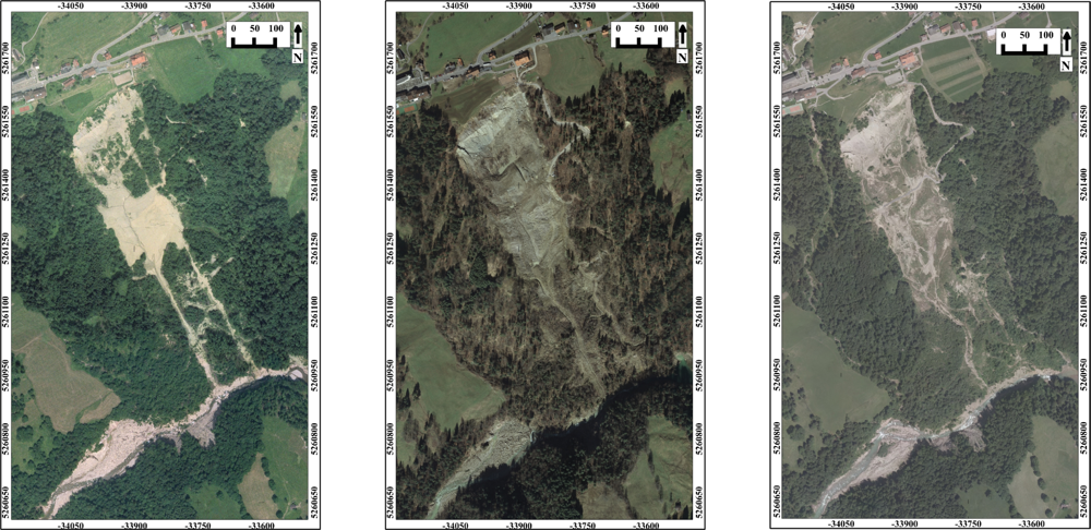
3.1. Study Site
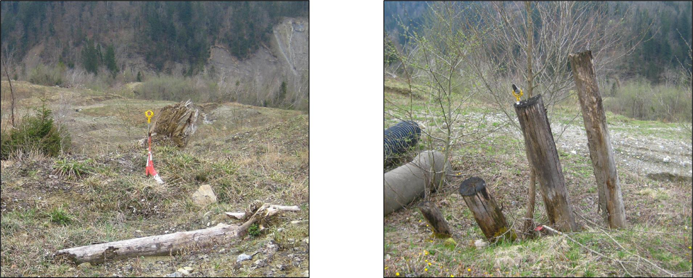
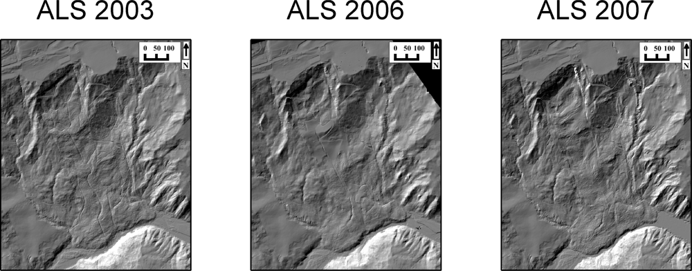
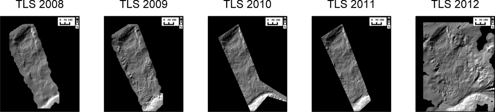
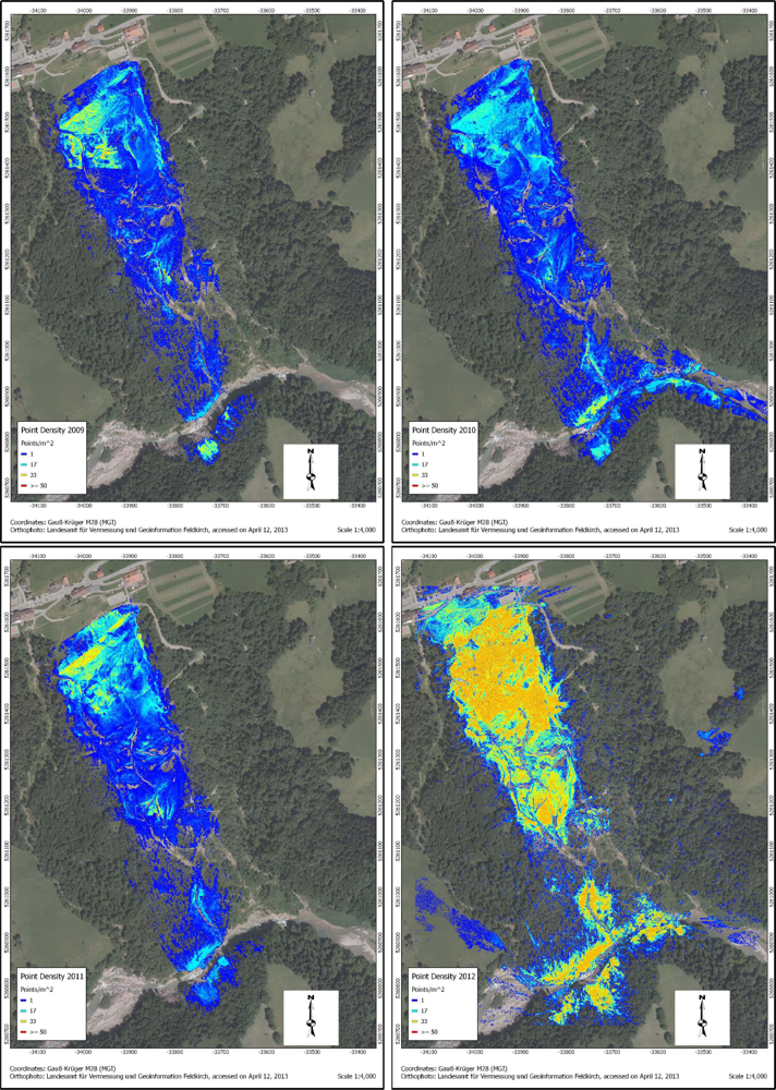
3.2. Data Acquisition and Basic Processing
3.3. Range Flow Methodology
3.4. Motion Detection Framework
4. Results
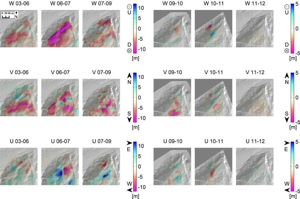
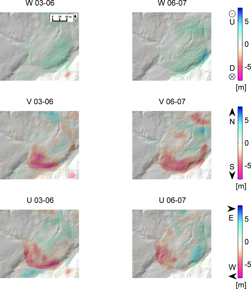
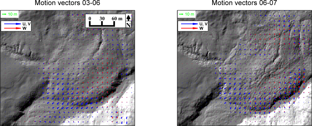
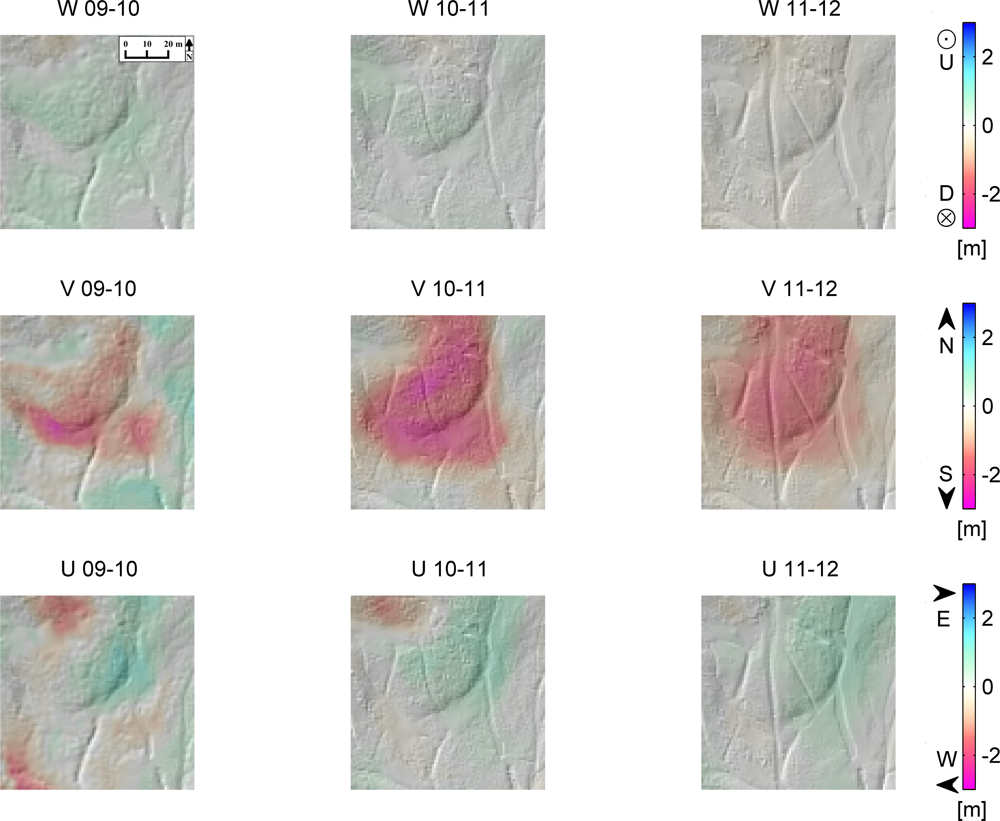
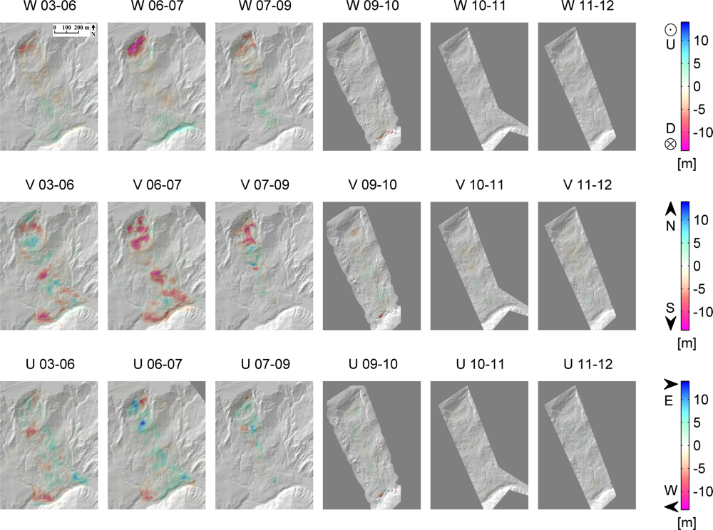
4.1. Flow Vectors
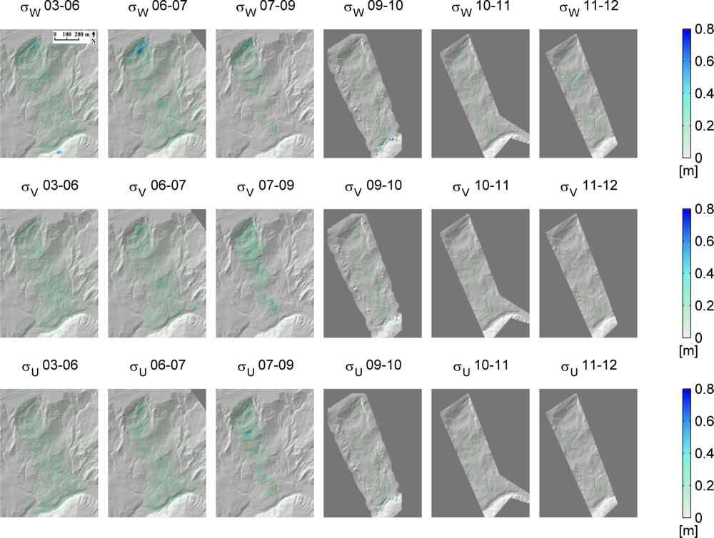
4.2. Interpretation and Assessment of the Results
4.3. Methodological Consequences
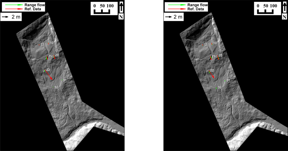
4.4. Comparison with Reference Data
5. Conclusions
Acknowledgments
- Conflict of InterestThe authors declare no conflict of interest.
References
- Kraus, K.; Pfeifer, N. Determination of terrain models in wooded areas with airborne laser scanner data. ISPRS J. Photogramm. 1998, 53, 193–203. [Google Scholar]
- Sithole, G.; Vosselman, G. Experimental comparison of filtering algorithms for bare-earth extraction from airborne laser scanning point clouds. ISPRS J. Photogramm. 2004, 59, 85–101. [Google Scholar]
- Horn, B.; Harris, J. Rigid body motion from range image sequences. CVGIP Image Underst. 1991, 53, 1–13. [Google Scholar]
- Yamamoto, M.; Boulanger, P.; Beraldin, J.; Rioux, M. Direct estimation of range flow on deformable shape from a video rate range camera. IEEE Trans. Patt. Anal. Mach. Intell. 1993, 15, 82–89. [Google Scholar]
- Spies, H.; Jahne, B.; Barron, J. Range flow estimation. Comput. Vision Image Underst. 2002, 85, 209–231. [Google Scholar]
- Bell, R.; Petschko, H.; Röhrs, M.; Dix, A. Assessment of landslide age, landslide persistence and human impact using airborne laser scanning digital terrain models. Geografiska Ann. Series A Phys. Geogr. 2012, 94, 135–156. [Google Scholar]
- Miller, P.; Kunz, M.; Mills, J.; King, M.; Murray, T.; James, T.; Marsh, S. Assessment of glacier volume change using ASTER-based surface matching of historical photography. IEEE Trans. Geosci. Remote Sens. 2009, 47, 1971–1979. [Google Scholar]
- Kenyi, L.; Kaufmann, V. Estimation of rock glacier surface deformation using SAR interferometry data. IEEE Trans. Geosci. Remote Sens. 2003, 41, 1512–1515. [Google Scholar]
- Tofani, V.; Raspini, F.; Catani, F.; Casagli, N. Persistent Scatterer Interferometry (PSI) technique for landslide characterization and monitoring. Remote Sens. 2013, 5, 1045–1065. [Google Scholar]
- Baldo, M.; Bicocchi, C.; Chiocchini, U.; Giordan, D.; Lollino, G. LIDAR monitoring of mass wasting processes: The Radicofani landslide, Province of Siena, Central Italy. Geomorphology 2009, 105, 193–201. [Google Scholar]
- Kasperski, J.; Delacourt, C.; Allemand, P.; Potherat, P.; Jaud, M.; Varrel, E. Application of a Terrestrial Laser Scanner (TLS) to the Study of the Séchilienne Landslide (Isère, France). Remote Sens. 2010, 2, 2785–2802. [Google Scholar]
- Dewitte, O.; Jasselette, J.; Cornet, Y.; Van Den Eeckhaut, M.; Collignon, A.; Poesen, J.; Demoulin, A. Tracking landslide displacements by multi-temporal DTMs: A combined aerial stereophotogrammetric and LiDAR approach in western Belgium. Eng. Geol. 2008, 99, 11–22. [Google Scholar]
- Feng, T.; Liu, X.; Scaioni, M.; Lin, X.; Li, R. Real-time Landslide Monitoring Using Close-Range Stereo Image Sequences Analysis. Proceedings of the 2012 International Conference on Systems and Informatics, Yantai, China, 19–20 May 2012; pp. 249–253.
- Lowe, D.G. Distinctive image features from scale-invariant keypoints. Int. J. Comput. Vision 2004, 60, 91–110. [Google Scholar]
- Aryal, A.; Brooks, B.A.; Reid, M.E.; Bawden, G.W.; Pawlak, G.R. Displacement fields from point cloud data: Application of particle imaging velocimetry to landslide geodesy. J. Geophys. Res.-Earth Surf. 2012. [Google Scholar] [CrossRef]
- Abdalati, W.; Krabill, W. Calculation of ice velocities in the Jakobshavn Isbrae area using airborne laser altimetry. Remote Sens. Environ. 1999, 67, 194–204. [Google Scholar]
- Schwalbe, E.; Maas, H. Motion analysis of fast flowing glaciers from multi-temporal terrestrial laser scanning (Bewegungsanalyse schnell fließender Gletscher aus multi-temporalen terrestrischen Laserscanneraufnahmen). Photogramm. Fernerkund. Geoinf. 2009, 2009, 91–98. [Google Scholar]
- Besl, P.; McKay, N. A method for registration of 3D shapes. IEEE Trans. Patt. Anal. Mach. Intell. 1992, 14, 239–256. [Google Scholar]
- Maas, H.; Casassa, G.; Schneider, D.; Schwalbe, E.; Wendt, A. Photogrammetric techniques for the determination of spatio-temporal velocity fields at Glaciar San Rafael, Chile. Photogramm. Eng. Remote Sensing 2013, 79, 299–306. [Google Scholar]
- Teza, G.; Galgaro, A.; Zaltron, N.; Genevois, R. Terrestrial laser scanner to detect landslide displacement fields: A new approach. Int. J. Remote Sens. 2007, 28, 3425–3446. [Google Scholar]
- Monserrat, O.; Crosetto, M. Deformation measurement using terrestrial laser scanning data and least squares 3D surface matching. ISPRS J. Photogramm. 2008, 63, 142–154. [Google Scholar]
- Grün, A.; Akca, D. Least squares 3D surface and curve matching. ISPRS J. Photogramm. 2005, 59, 151–174. [Google Scholar]
- Kraus, K.; Ressl, C.; Roncat, A. Least Squares Matching for Airborne Laser Scanner Data. Proceedings of the 5th International Symposium Turkish-German Joint Geodetic Days, Berlin, Germany, 29–31 March 2006; p. 7.
- Jaboyedoff, M.; Oppikofer, T.; Abellán, A.; Derron, M.; Loye, A.; Metzger, R.; Pedrazzini, A. Use of LIDAR in landslide investigations: A review. Nat. Hazards 2012, 61, 5–28. [Google Scholar]
- Marr, D. Vision: A Computational Investigation into the Human Representation and Processing of Visual Information; Henry Holt and Co., Inc.: New York, NY, USA, 1982. [Google Scholar]
- Horn, B.; Schunck, B. Determining optical flow. Artif. Intell. 1981, 17, 185–203. [Google Scholar]
- Gottfried, J.; Fehr, J.; Garbe, C. Computing Range Flow from Multi-Modal Kinect Data. In Advances in Visual Computing; Bebis, G., Boyle, R., Parvin, B., Koracin, D., Wang, S., Kyungnam, K., Benes, B., Moreland, K., Borst, C., DiVerdi, S., et al., Eds.; Springer: Berlin/Heidelberg, Germany, 2011; pp. 758–767. [Google Scholar]
- Schuchert, T.; Aach, T.; Scharr, H. Range Flow for Varying Illumination. In Computer Vision–ECCV 2008; Forsyth, D., Torr, P., Zisserman, A., Eds.; Springer: Berlin/Heidelberg, Germany, 2008; pp. 509–522. [Google Scholar]
- Ghuffar, S.; Brosch, N.; Pfeifer, N.; Gelautz, M. Motion Segmentation in Videos from Time of Flight Cameras. Proceedings of the 19th International Conference on Systems, Signals and Image Processing, Vienna, Austria, 11–13 April 2012; pp. 328–332.
- Zhang, Z. Iterative point matching for registration of free-form curves and surfaces. Int. J. Comput. Vision 1994, 13, 119–152. [Google Scholar]
- Ressl, C.; Pfeifer, N.; Mandlburger, G. Appyling 3D affine transformation and least squares matching for airborne laser scanning strips adjustment without GNSS/INS trajectory data. Int. Arch. Photogramm. Remote Sens. Spat. Inf. Sci. 2011, 38. [Google Scholar] [CrossRef]
- Spies, H.; Haußecker, H.; Jähne, B.; Barron, J. Differential Range Flow Estimation. Proceedings of the German Association for Pattern Recognition Symposium, Bonn, Germany, 15–17 September 1999; pp. 309–316.
- Ressl, C.; Kager, H.; Mandlburger, G. Quality checking of ALS projects using statistics of strip differences. Int. Arch. Photogramm. Remote Sens. Spat. Inf. Sci. 2008, 37, 253–260. [Google Scholar]
- Rusinkiewicz, S.; Levoy, M. Efficient Variants of the ICP Algorithm. Proceedings of the Third International Conference on 3-D Digital Imaging and Modeling (3DIM ’01), Quebec City, QC, Canada, 28 May–1 June 2001; pp. 145–152.
- Glazer, F.C. Hierarchical Motion Detection. 1987. [Google Scholar]
- Brox, T.; Bruhn, A.; Papenberg, N.; Weickert, J. High Accuracy Optical Flow Estimation Based on a Theory for Warping. In Computer Vision-ECCV 2004; Pajdla, T., Matas, J., Eds.; Springer: Berlin/Heidelberg, Germany, 2004; pp. 25–36. [Google Scholar]
- Mikhail, E.M. Observations and Least Squares; IEP-A Dun-Donnelley: New York, NY, USA, 1976. [Google Scholar]
- New, M.; Lister, D.; Hulme, M.; Makin, I. A high-resolution data set of surface climate over global land areas. Clim. Res. 2002, 21, 1–25. [Google Scholar]
- van Husen, D. Die Ostalpen in den Eiszeiten; Geologische Bundesanstalt: Vienna, Austria, 1987; p. 24. [Google Scholar]
- Herrmann, P.; Draxler, I.; Müller, M. Geologische Karte der RepublikÖsterreich 1:25.000. Erläuterungen zu Blatt 83 Sulzberg; Geologische Bundesanstalt: Vienna, Austria, 1985; p. 21. [Google Scholar]
- Czurda, K.A.; Ginther, G. Quellverhalten der molassemergel im pfänderstock bei bregenz, österreich (expansion behaviour of molasse-marls of the pfänder near Bregenz/Austria). Mitteilungen der Österreichischen Geologischen Gesellschaft 1983, 76, 141–160. [Google Scholar]
- Zámolyi, A.; Székely, B.; Biszak, S. Assessing the accuracy of the second military survey for the Doren landslide (Vorarlberg, Austria). Geophys. Res. Abstr. 2010, 12, 9974. [Google Scholar]
- Drexel, P.; Seebacher, M. Einmal ist Keinmal–die Anwendung von Luftbild-/Laserscanning-/Geodatenzeitreihen in der Vorarlberger Landesverwaltung. In 17 Internationale Geodätische Woche Obergurgl 2013; Hanke, K., Weinold, T., Eds.; Wichmann Verlag: Berlin/Offenbach, Germany, 2013; pp. 50–55. [Google Scholar]
- Roncat, A.; Dorninger, P.; Molnár, G.; Székely, B.; Zámolyi, A.; Melzer, T.; Pfeifer, N.; Drexel, P. Influences of the Acquisition Geometry of different Lidar Techniques in High-Resolution Outlining of Microtopographic Landforms. In Fachtagung Computerorientierte Geologie–COGeo 2010; Marschallinger, R., Wanker, W., Zobl, F., Eds.; Arbeitsgruppe Computerorientierte Geologie derÖsterreichischen Geologischen Gesellschaft: Salzburg, Austria, 2010. [Google Scholar]
- SCOP++. Institute of Photogrammetry and Remote Sensing. 2013. Available online: www.ipf.tuwien.ac.at/products/products.html (accessed on 23 May 2013).
- OPALS. Institute of Photogrammetry and Remote Sensing. 2013. Available online: www.ipf.tuwien.ac.at/opals (accessed on 23 May 2013).
- Pfeifer, N.; Mandlburger, G. Filtering and DTM Generation. In Topographic Laser Ranging and Scanning: Principles and Processing; Shan, J., Toth, C.K., Eds.; CRC Press: Boca Raton, FL, USA, 2008; pp. 307–334. [Google Scholar]
- Snow, K.B. Topics in Total Least-Squares Adjustment within the Errors-In-Variables Model: Singular Cofactor Matrices and Prior Information. 2012. [Google Scholar]
- Baker, S.; Scharstein, D.; Lewis, J.; Roth, S.; Black, M.; Szeliski, R. A database and evaluation methodology for optical flow. Int. J. Comput. Vision 2011, 92, 1–31. [Google Scholar]
- Brox, T.; Malik, J. Large displacement optical flow: Descriptor matching in variational motion estimation. IEEE Trans. Pattern Anal. Mach. Intell. 2011, 33, 500–513. [Google Scholar]
- Guarnieri, A.; Pirotti, F.; Vettore, A. Comparison of discrete return and waveform terrestrial laser scanning for dense vegetation filtering. Int. Arch. Photogramm. Remote Sens. Spat. Inf. Sci. 2012, 39, 511–516. [Google Scholar]
- Mittelberger, M. Vom Nutzen bewegter “Fest” punkte und “verrückter” Grenzen. In 16 Internationale Geodätische Woche Obergurgl 2011; Grimm-Pitzinger, A., Weinold, T., Eds.; Wichmann Verlag: Berlin/Offenbach, Germany, 2011; pp. 85–89. [Google Scholar]


| Pts. | Range Flow 10–11 (m) | Ref. Vector 10–11 (m) | Difference 10–11 (m) | Range Flow 11–12 (m) | Ref. Vector 11–12 (m) | Difference 11–12 (m) |
|---|---|---|---|---|---|---|
| #10 | −0.15, −0.11, −0.10 | 0.10, −0.49, −0.02 | −0.26, 0.38, −0.08 | 0.28, −0.59, −0.14 | 0.11, −0.56, 0.00 | 0.17, −0.02, −0.14 |
| #11 | 0.15, −0.16, 0.46 | 0.05, −0.32, −0.16 | 0.10, 0.17, 0.62 | 0.05, −0.38, −0.07 | 0.06, −0.35, −0.15 | −0.01, −0.03, 0.08 |
| #20 | 0.22, −0.86, −0.32 | 0.38, −1.31, −0.32 | −0.16, 0.46, 0.01 | 0.64, −1.26, −0.46 | 0.48, −1.41, −0.33 | 0.16, 0.15, −0.13 |
| #21 | −0.14, −1.15, −0.35 | 0.31, −1.10, −0.27 | −0.44, −0.05, −0.08 | 0.55, −0.69, −0.46 | 0.35, −1.20, −0.21 | 0.21, 0.50, −0.25 |
| #22 | −0.20, −0.58, −0.01 | 2.41, −3.32, −0.21 | −2.61, 2.74, 0.20 | 0.41, −0.84, −0.25 | 1.76, −2.56, 0.05 | −1.34, 1.72, −0.31 |
| #31 | 0.23, 0.23, 0.14 | −0.00, −0.03, −0.00 | 0.24, 0.26, 0.14 | −0.08, −0.36, −0.07 | −0.01, −0.03, 0.00 | −0.07, −0.33, −0.08 |
| #32 | 0.07, 0.07, 0.21 | 0.01, −0.03, −0.00 | 0.06, 0.10, 0.22 | −0.01, −0.29, −0.13 | 0.01, −0.03, 0.00 | −0.02, −0.26, −0.13 |
© 2013 by the authors; licensee MDPI, Basel, Switzerland This article is an open access article distributed under the terms and conditions of the Creative Commons Attribution license (http://creativecommons.org/licenses/by/3.0/).
Share and Cite
Ghuffar, S.; Székely, B.; Roncat, A.; Pfeifer, N. Landslide Displacement Monitoring Using 3D Range Flow on Airborne and Terrestrial LiDAR Data. Remote Sens. 2013, 5, 2720-2745. https://doi.org/10.3390/rs5062720
Ghuffar S, Székely B, Roncat A, Pfeifer N. Landslide Displacement Monitoring Using 3D Range Flow on Airborne and Terrestrial LiDAR Data. Remote Sensing. 2013; 5(6):2720-2745. https://doi.org/10.3390/rs5062720
Chicago/Turabian StyleGhuffar, Sajid, Balázs Székely, Andreas Roncat, and Norbert Pfeifer. 2013. "Landslide Displacement Monitoring Using 3D Range Flow on Airborne and Terrestrial LiDAR Data" Remote Sensing 5, no. 6: 2720-2745. https://doi.org/10.3390/rs5062720
APA StyleGhuffar, S., Székely, B., Roncat, A., & Pfeifer, N. (2013). Landslide Displacement Monitoring Using 3D Range Flow on Airborne and Terrestrial LiDAR Data. Remote Sensing, 5(6), 2720-2745. https://doi.org/10.3390/rs5062720