Article

Using Satellite Data to Represent Tropical Instability Waves (TIWs)-Induced Wind for Ocean Modeling: A Negative Feedback onto TIW Activity in the Pacific

1
Key Laboratory of Meteorological Disaster of Ministry of Education, Nanjing University of Information Science and Technology, Nanjing 210044, China
2
Earth System Science Interdisciplinary Center (ESSIC), University of Maryland, College Park, MD 20740, USA
*
Author to whom correspondence should be addressed.
Remote Sens. 2013, 5(6), 2660-2687; https://doi.org/10.3390/rs5062660
Submission received: 2 April 2013 / Revised: 20 May 2013 / Accepted: 20 May 2013 / Published: 24 May 2013

Abstract

:
Recent satellite data and modeling studies indicate a pronounced role Tropical Instability Waves (TIW)-induced wind feedback plays in the tropical Pacific climate system. Previously, remotely sensed data were used to derive a diagnostic model for TIW-induced wind stress perturbations (τTIW), which was embedded into an ocean general circulation model (OGCM) to take into account TIW-induced ocean-atmosphere coupling in the tropical Pacific. While the previous paper by Zhang (2013) is concerned with the effect on the mean ocean state, the present paper is devoted to using the embedded system to examine the effects on TIW activity in the ocean, with τTIW being interactively determined from TIW-scale sea surface temperature (SSTTIW) fields generated in the OGCM, written as τTIW = αTIW·F(SSTTIW), where αTIW is a scalar parameter introduced to represent the τTIW forcing intensity. Sensitivity experiments with varying αTIW (representing TIW-scale wind feedback strength) are performed to illustrate a negative feedback induced by TIW-scale air-sea coupling and its relationship with TIW variability in the ocean. Consistent with previous modeling studies, TIW wind feedback tends to have a damping effect on TIWs in the ocean, with a general inverse relationship between the τTIW intensity and TIWs. It is further shown that TIW-scale coupling does not vary linearly with αTIW: the coupling increases linearly with intensifying τTIW forcing at low values of αTIW (in a weak τTIW forcing regime); it becomes saturated at a certain value of αTIW; it decreases when αTIW goes above a threshold value as the τTIW forcing increases further. This work presents a clear demonstration of using satellite data to effectively represent TIW-scale wind feedback and its multi-scale interactions with large-scale ocean processes in the tropical Pacific.

1. Introduction

Tropical instability waves (TIWs) are intraseasonal, small-scale phenomena in the central-eastern tropical Pacific which were first revealed from remotely sensed image [1]. As has been recognized for a long time [26], TIWs are an important component in the tropical Pacific climate system, exerting an influence on the ocean through their contributions to heat and momentum transports near the equator [710]. For example, as demonstrated from satellite measurements [11], atmospheric surface winds over the eastern tropical Pacific exhibit coherent relationships with sea surface temperatures (SSTs), inducing a wind feedback onto the ocean and thus coupled air–sea interactions on TIW scales. Due to the large magnitude of TIW-induced wind and SST perturbations, it is necessary to adequately take into account TIW-scale wind forcing and its feedback effect on large-scale climate modeling.
The challenge to represent TIW-induced wind feedback is due to the fact that high-resolution coupled general circulation models (GCMs) (that can resolve small-scale signals associated with TIWs) are not developed realistically enough and their extensive uses are not affordable in long-term coupled climate system modeling context. At present, adequately representing TIW-induced wind feedback in global climate models is still a difficult task since vastly different space-time scales are involved, with great uncertainties in accurately depicting TIW-scale surface wind responses and its coupling with SSTs.
Over the past decades, microwave remote sensing has made great progress in observing and describing these TIW-scale processes over the tropical oceans [12,13]. For example, SSTs can be now measured with unprecedented accuracy by the Tropical Rain Measuring Mission (TRMM) satellite’s microwave imager [11,14,15]; the SeaWinds Scatterometer on the QuikSCAT satellite can also provide accurate observations of sea surface vector winds [16,17]. These high quality satellite data can now resolve TIW-linked small-scale signals both in the atmosphere and in the ocean. In particular, a coherent co-variability pattern between TIW-scale surface winds and SSTs has been depicted over the eastern tropical Pacific [11,12,18]. These microwave measurements have led to significant advances in physical understanding, interpretation and modeling efforts of TIW-scale air–sea interactions over the tropical Pacific. For example, Zhang and Busalacchi [19] used historical satellite data to develop a simple empirical model for TIW-induced surface wind stress perturbations (τTIW). When being embedded into a basin-scale ocean model, the statistically derived τTIW model serves as an atmospheric component to form an internally coupled wind-SST subsystem on TIW scales. Without making use of a comprehensive atmospheric model that can resolve TIW variability in a computationally intensive way, this embedded modeling system allows one to decipher the impact of TIW-induced wind feedback on the ocean, and further its interactions with seasonal and interannual variations over the tropical Pacific.
In a previous modeling study [20], we examined the effects of TIW-induced wind (τTIW) forcing on the mean state using a basinwide ocean model of the tropical Pacific and the empirically derived model for τTIW. One main result from this ocean-only modeling study was that the TIW-induced wind can have a cooling effect on SST in the eastern equatorial Pacific. In addition, as TIW-induced SST perturbations emerge in the region, surface wind responses are induced instantly and coherently on TIW scales, which exert an influence back on TIWs in the ocean, leading to an ocean-atmosphere coupling at TIW scales. This indicates that TIW activity in the ocean can be also modulated by TIW-induced wind and the related feedback and coupling.
Some previous studies have shown that TIWs in the ocean tend to be damped by TIW-induced wind feedback via various processes, including SST-wind-current coupling, Ekman pumping and thermal dampening. For example, Seo et al. [21] identified an anti-correlation pattern between TIW-induced perturbations of surface current and wind stress, which can serve as a negative feedback having a diminishing impact on TIWs in the ocean. Also, Pezzi et al. [22] showed that when TIW wind forcing is explicitly included, TIWs decrease in the ocean. Small et al. [23] illustrated another negative feedback involved with ocean current-induced effects on surface wind stress using a regionally fully coupled ocean-atmosphere model over the eastern tropical Pacific.
Understanding the way TIW activity in the ocean is modulated by TIW-scale wind is important since TIWs directly affect the mixed layer heat budget and thus SST in the eastern tropical Pacific, a region where the El Niño-Southern Oscillation (ENSO) is generated and has effects on weather and climate patterns worldwide. For example, the meridional heat advection associated with TIWs tends to warm the upper equatorial ocean [4,7]. It follows that when TIWs in the ocean become weaker as a result of TIW-induced wind effect, the warming effect from the meridional heat advection is reduced in the eastern equatorial Pacific, which can be responsible for the mean state cooling [20]. Also, high-frequency TIW wind forcing directly affects vertical mixing in the upper ocean, leading to an increase in its cooling effect on SSTs [24,25]. Thus, there are close connections among TIW-induced wind forcing and feedback, TIW activity in the ocean, the mixed-layer heat budget and SST. In addition, TIW activity in the ocean is modulated by large-scale climate conditions in the eastern tropical Pacific, which are observed to undergo prominent seasonal and interannual variations [26]. Clearly, TIW-induced wind effects involve multi-process interactions on TIW, seasonal and interannual scales in the tropical Pacific climate system.
At present, the sensitivity of TIW activity in the ocean to the way TIW-induced wind feedback is represented is poorly understood, and the relationships among TIW-scale wind forcing, the related feedback and coupling, and SST in the tropical Pacific have not been quantified. While a fully coupled ocean-atmosphere model with high resolution can be used to depict TIW-scale wind variability in the region [20,2729], it is difficult to unambiguously isolate TIW-induced feedback effects since all related multi-scale processes are present together, with their effects intermingled. Also, adequately resolving atmospheric wind responses to TIW-induced SST forcing requires a high-resolution model, which is computationally intensive.
In this paper, we continue to examine the effects of TIW-induced wind feedback in an ocean-only modeling context, with a focus on TIW activity in the ocean and the related ocean-atmosphere coupling at TIW scales. As with [21], a SST-dependent model for TIW-induced wind stress perturbations (τTIW) is derived using satellite observations [19,30], which is incorporated into a basin-wide ocean general circulation model (OGCM) of the tropical Pacific. As will be seen below, this empirical τTIW modeling approach can reasonably well depict TIW-scale coupling between the ocean and atmosphere in the eastern tropical Pacific. In addition, the τTIW forcing intensity can be conveniently adjusted using this embedded modeling system, allowing to quantify its effects on the ocean in a flexible way.
Based on this computationally efficient modeling framework, numerical simulations with varying TIW wind feedback intensity are compared to quantify its effects on TIW activity in the ocean. The following specific questions are addressed. How do TIWs in the ocean respond to TIW-induced wind feedback and to its intensity changes? Are TIWs weakened or enhanced when the τTIW forcing effect is interactively included? What are the relationships between TIW-scale coupling intensity and TIW activity in the ocean? How do the effects and relationships change with the τTIW forcing intensity?
The paper is organized as follows. Section 2 briefly describes the model components used in representing TIW-induced wind effects. The effects on TIW activity in the ocean are analyzed and compared with each other in Sections 3 and 4 for a no-feedback run and a reference feedback run, respectively. In Section 5, a discussion is presented with further experiments performed to examine the sensitivity to changes in the τTIW forcing intensity. A conclusion is given in Section 6.

2. Model and Experiment Designs

As illustrated in Figure 1 and detailed in [20], we use a simple embedded modeling system, which consists of a basin-scale OGCM of the tropical Pacific and a simple statistical feedback model for TIW-induced wind stress perturbations (τTIW) over the central-eastern tropical Pacific. In this ocean-only modeling context, the total wind stress fields to force the OGCM can be separated into its climatological (τclim) and TIW-scale (τTIW) parts, written as τ = τclim + τTIW. In this section, we briefly describe these various components and model experiment designs.
The OGCM used is the reduced gravity, primitive equation, sigma-coordinate model of [31], which is developed specifically for studying the coupling between the dynamics and thermodynamics of the upper tropical ocean. The vertical structure of the ocean model consists of a mixed layer and a number of layers below which are specified according to a sigma-coordinate. The mixed layer depth and the thickness of the last sigma layer are computed prognostically. Several related efforts have improved this ocean model significantly. Chen et al. [32] developed a hybrid mixed layer model which was embedded into the OGCM. Murtugudde et al. [33] coupled the OGCM to an advective atmospheric mixed layer (AML) model to estimate sea surface heat fluxes and showed a non-local effect of the atmospheric boundary layer on SST. This heat flux parameterization allows a realistic representation of the feedbacks between mixed layer depths, SSTs, and the surface heat fluxes. Additionally, the effect of penetrative radiation on the upper tropical ocean has been taken into account, with attenuation depths derived from remotely sensed ocean color data [34]. These process-oriented studies have improved simulations of ocean circulation and thermal structure significantly. More recent efforts with this OGCM include the developments of a hybrid coupled ocean-atmosphere model (HCM) for the tropical Pacific [35], and its applications to representing and understanding various feedback effects in the tropical Pacific climate system [36,37]. The OGCM domain covers the tropical Pacific basin from 25°S to 25°N and from 124°E to 76°W, with horizontal resolution of 1° longitude and of 0.5° latitude, and with 31 layers in the vertical. Sponge layers are imposed near the model southern and northern boundaries (poleward of 20°S/N). The OGCM is initiated from the WOA01 temperature and salinity fields, and is integrated for 20 years using prescribed atmospheric climatological forcing fields.
An empirical model for τTIW was constructed from historical satellite data using a singular vector decomposition (SVD) analysis technique [19] for an 8-year period from 2000 to 2007. Daily data of SST are from the TRMM microwave imager (TMI) measurements [14]; those of wind stress are from the QuikSCAT scatterometer observations [16]. To extract TIW-scale signals in the ocean and atmosphere, a spatial high-pass filter (by subtracting a 12° zonal moving average from the original data) is applied to daily data of SST and wind stress to remove large-scale background fields. The resultant spatially high-pass filtered data have a horizontal resolution of 1° in longitude and of 0.5° in latitude. Figure 2(a,b) illustrates examples for total SST and SSTTIW fields on 1 October 1999 derived from the satellite data. TIW signals are clearly evident in the eastern tropical Pacific.
The derived daily SSTTIW and τTIW fields over the 8-year period are then used to perform a combined SVD analysis to determine their statistically optimized dominant modes. Due to computational limitations in performing SVD calculations, the SVD analysis domain is confined to the central-eastern tropical Pacific from 15°S to 15°N and from 180° to 76°W, which is an active TIW region. From this SVD analysis, an empirical relationship between τTIW and SSTTIW is constructed using the derived dominant SVD modes, symbolically written as τTIW = αTIW·F(SSTTIW), where F represents the SVD-determined empirical relationships between SSTTIW and τTIW, and a scalar parameter, αTIW, is introduced to represent TIW-scale wind feedback intensity.
Figure 3 exhibits the spatial structure of the first SVD mode for the SSTTIW and τTIW (the zonal and meridional components) fields derived from the satellite data. As analyzed in [19], the covariance between τTIW and SSTTIW accounted for by each SVD mode is quite small in the combined SVD analyses. For example, the first 10 modes account for only about 36% of the covariance. Thus, more than half of the covariance is lost when using this empirical τTIW model to construct a τTIW response to a given SSTTIW field. Figure 2(c,d) presents an example for the derived zonal and meridional τTIW components from a given SSTTIW field using this empirical model with αTIW = 1.0 taken and the 10 SVD modes retained. It is clearly evident that the τTIW amplitude simulated is significantly underestimated compared with that observed from the corresponding satellite. The so-called rescaling factor, αTIW, is introduced that can provide an effective way to improve the τTIW amplitude simulation [19]. That is, this parameter can be adjusted (generally taken to be larger than 1) in such a way that the calculated τTIW amplitude matches observed one [19,35]. Testing experiments indicate that the amplitude and structure of τTIW can be both reasonably well depicted from SSTTIW simulated in the OGCM using this empirical model with αTIW = 3.0 taken and the 10 SVD modes retained.
The empirical τTIW model is embedded into the OGCM; a daily τTIW-SSTTIW coupling is implemented as follows. At each time step, the OGCM calculates SST fields, which are averaged to obtain its daily-mean values, from which TIW-scale SST perturbations are extracted using the spatial high-pass filter described above. The resultant SSTTIW fields are then used to diagnostically determine τTIW, which is added onto the τclim field to force the OGCM. The interactively represented TIW wind part is applied only to the central-eastern tropical Pacific between 15°N and 15°S, and east of the date line. Note that as τTIW is interactively determined from SSTTIW simulated in the OGCM, the ocean-atmosphere coupling at TIW scales is internally depicted over the central-eastern tropical Pacific, even though an ocean-only model is used.
The OGCM experiments are performed with varying values of αTIW to represent TIW wind feedback intensity. A no-feedback run is conducted in which TIW-scale wind part is not taken into account (αTIW = 0.0). Then, a reference feedback run is performed in which the τTIW forcing part is interactively taken into account using its empirical model with αTIW = 3.0 taken and the first 10 SVD modes retained. Additionally, several other experiments are analyzed with αTIW = 1.0 and αTIW = 2.0 (the TIW wind feedback being weakly represented) and αTIW = 4.0 (the TIW wind feedback being strongly represented), respectively. Started from the long-term spin-up state, the OGCM is additionally integrated for 13 years, with daily outputs being saved. To represent TIW signals, daily fields from one individual year (the 13th year) are used to analyze TIW activity in the ocean and the related ocean-atmosphere coupling at TIW scales.

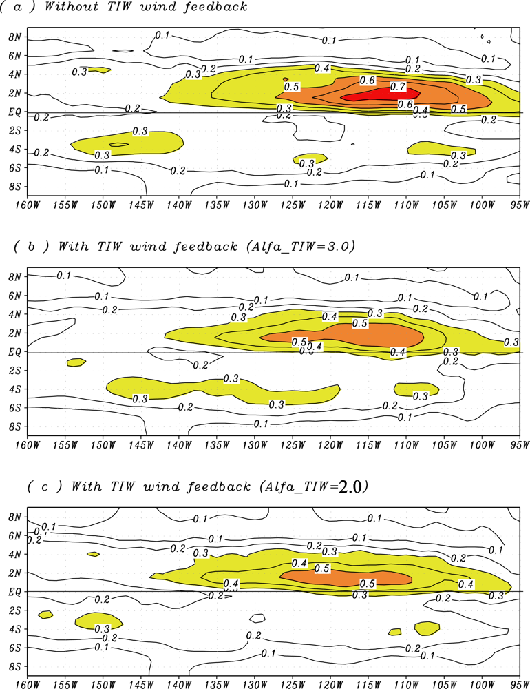
3. A No-Feedback Run (αTIW = 0.0)

One experiment is performed in which the OGCM is forced by monthly-mean climatological winds only, referred as a no-feedback run (αTIW = 0.0). The simulated daily fields for total SSTs show clear TIW signals in the eastern tropical Pacific Ocean, which are generated internally in the OGCM. To extract TIW-scale perturbations, a spatial high-pass filter (by the subtracting of a 12° zonal moving average) is applied to simulated daily SST fields. Figure 4(a) shows an example of seasonal variations of the TIW-scale SST perturbations in the no-feedback run. Vigorous TIW signals are seen in the eastern basin, with a coherent westward propagation and seasonal modulation; TIWs are strong during cold seasons, but weak during warm seasons.
As a measure of TIW strength, the spatial distribution of the standard deviation (sdv) for SSTTIW is shown in Figure 5. The largest SSTTIW variability center is located in the TIW active region over the eastern equatorial Pacific; the spatially averaged sdv of SSTTIW is about 0.42 °C in the region (150°W–105°W, 0–5°N). The sdv of SSTTIW exhibits a clear seasonal variation (Figure 6(a)), with large sdv values taking place from September to December when TIWs are strong in the ocean. The strength of TIWs in the ocean can also be measured by the eddy kinetic energy (EKE) which is calculated using the zonal-high-pass filtered currents in the surface mixed layer, defined as:
ρ 0 2 ( u TIW 2 + v TIW 2 )
Figures 6(c) and 7(a) show the EKE computed from the no-feedback run. Large EKE region is located in the central-eastern equatorial Pacific, with a maximum in the longitude range from 150°W to 135°W. The regionally averaged EKE is about 18 kg·m−1·s−2 from 100°W to 160°W and from the equator to 5°N. While the maximum sdv center of SSTTIW is located around 120°W (Figure 5(a)), that of the EKE exhibits a westward shift to around 150°W–140°W (Figure 7(a)).

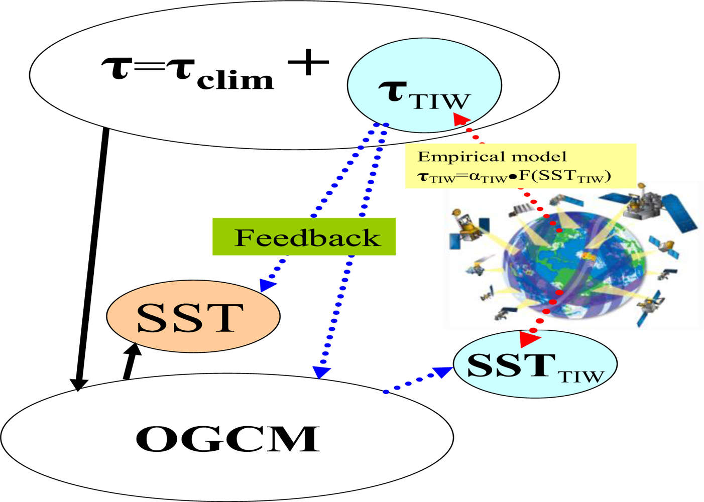
4. The Effects of Tropical Instability Wave (TIW)-Induced Wind Feedback: A Reference Feedback Run

Next, a reference feedback run (αTIW = 3.0) is conducted in which the τTIW feedback is interactively represented, with other model settings being kept exactly the same as in the no-feedback run. When τTIW is determined using SSTTIW simulated from the OGCM, the τTIW forcing induces TIW-scale coupling between the ocean and atmosphere: the TIW-scale wind feedback acts to have a modulating effect on SSTTIW, which exerts an influence back on τTIW. In this section, daily outputs from the OGCM simulation in year 13 are used to investigate the τTIW feedback effects on TIW activity in the ocean and the related TIW-scale coupling between the ocean and atmosphere.

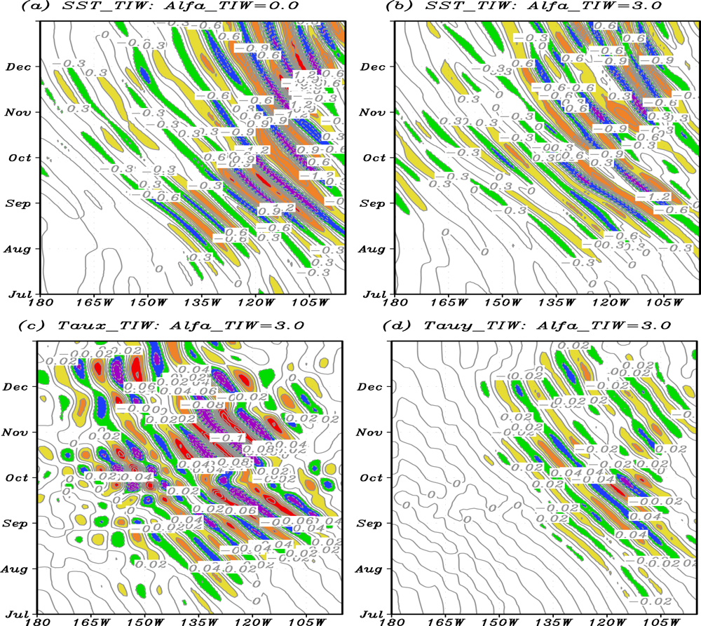
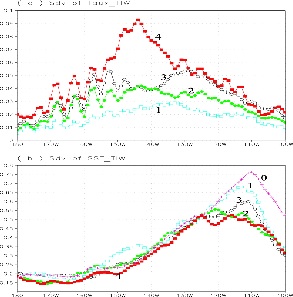
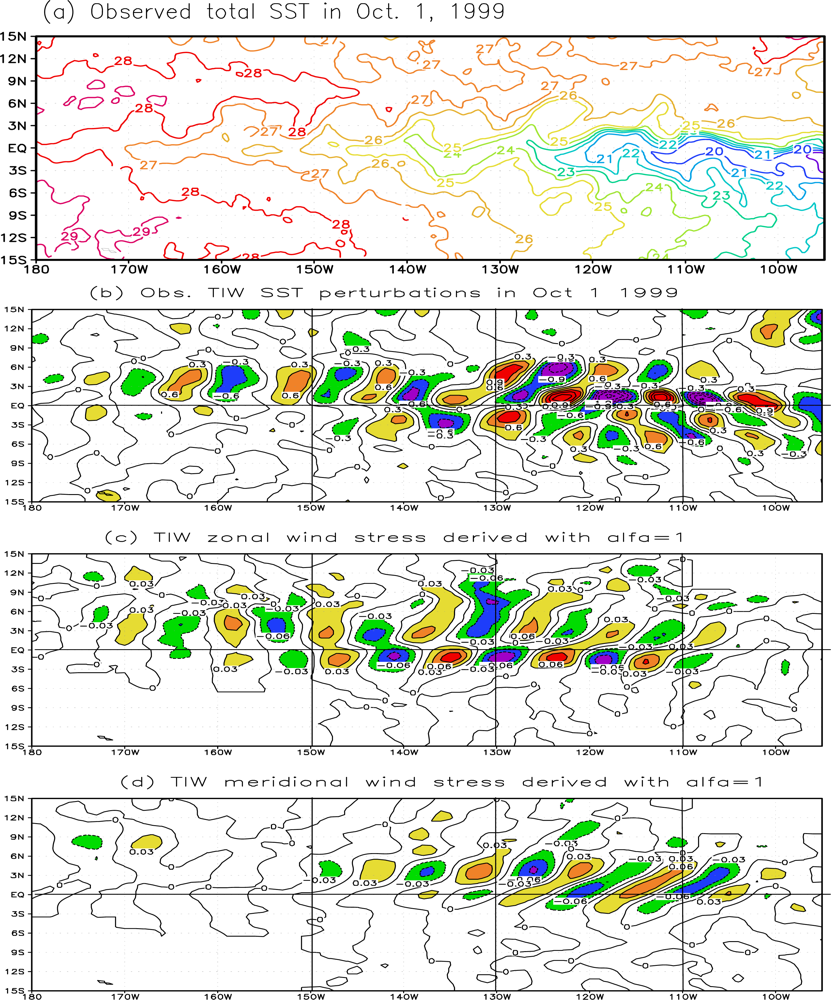
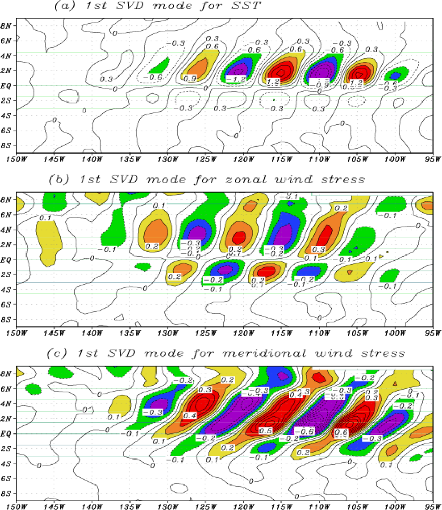
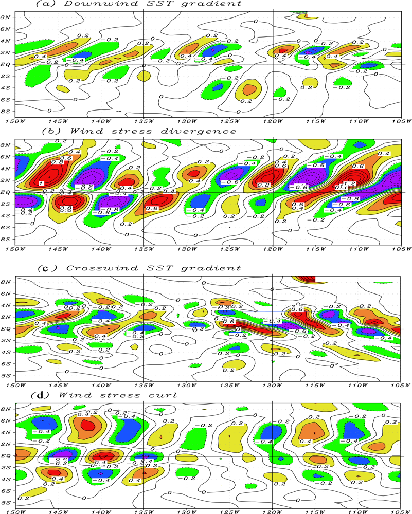
4.1. TIW-Scale Perturbations of SST and Surface Wind Stress

Spatial structure and seasonal variations of simulated TIW-scale perturbations in the reference feedback run are shown in Figures 4, 5, 6 and 7. For example, the SSTTIW signals are prominent in the eastern equatorial Pacific, with clear seasonal modulations (Figure 4(b)). The corresponding τTIW fields derived from the SSTTIW fields show coherent TIW-scale signals, being predominantly present only in regions where TIW-induced SST perturbations exist. A co-variability pattern is clearly seen between the SSTTIW (Figure 4(b)) and τTIW fields over the eastern tropical Pacific (Figure 4(c,d)); their corresponding horizontal patterns can be typically represented in the 1st SVD mode as indicated in Figure 3. For example, surface winds accelerate (decelerate) when blowing across positive (negative) SSTTIW regions, which was analyzed in detail in [19]. As a measure of TIW activity, the spatial distribution and seasonal variation of the sdv for SSTTIW are shown in Figures 5(b) and 6(b). The sdv of SSTTIW calculated in the region (150°W–105°W, 0°N–5°N) is 0.35 °C in the reference feedback run.

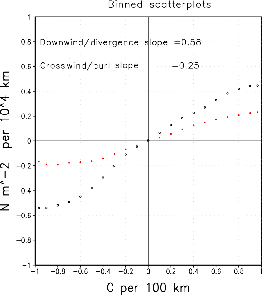
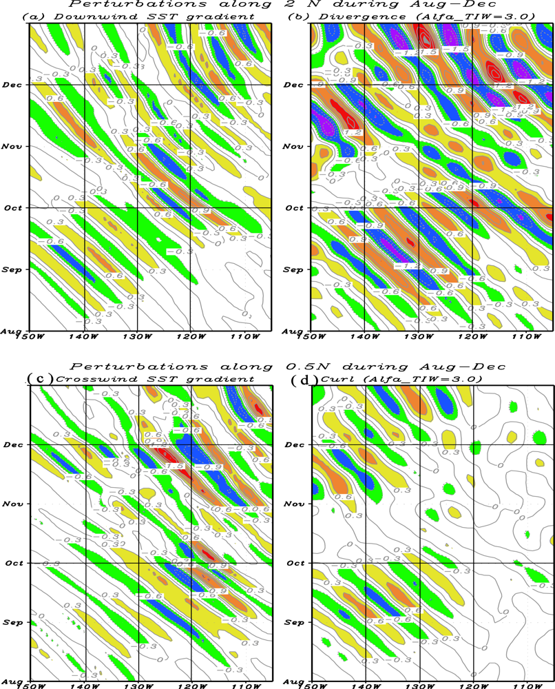
4.2. The Ocean-Atmosphere Coupling at TIW Scales

As demonstrated by [11], the TIW-induced ocean-atmosphere coupling can be most clearly manifest in the wind stress divergence and curl fields. Following [11], the zonal-high-pass filtered downwind and crosswind components of the SST gradient are respectively written as
( SST τ / | τ | ) and ( SST × τ / | τ | ) k
where τ = τclim + τTIW, and k⃗ is a unit vector in the vertical direction. Using the outputs simulated from the OGCM, these parameters are estimated to represent TIW-scale coupling between the ocean and atmosphere, including the divergence and curl fields, and the corresponding downwind and crosswind components of the SST gradient.
Figures 8 and 9 illustrate examples of the spatial patterns and seasonal evolutions of the divergence and curl fields derived from the reference feedback run. The TIW-scale divergence and curl signals are most pronounced over the eastern equatorial Pacific, with their coherent patterns with SSTTIW. For example, when the winds blow across the positive (negative) SSTTIW regions and get accelerated (decelerated), they converge north of the warm SSTTIW region and diverge south of the cold SSTTIW region. As a result, the prolonged bands of strong wind stress divergence are induced to the northeast-southwest, with the most intensive centers being locally overlapped with the zonally banded SSTTIW regions. Also, the horizontal variations in the wind response generate positive/negative curl bands, which are most intensive non-locally to the west and to the east of the SSTTIW centers, shifted zonally by a quarter of wavelength. Thus, geographical locations of the divergence and curl maxima show clear differences in their spatial relationship with the SSTTIW forcing centers. It is also evident that these two derived fields exhibit different response amplitude, with the divergence perturbations being more pronounced and coherent than the curl ones [11]. This indicates that TIW-induced SSTTIW forcing acts to have the effects that are stronger on divergence than on curl [38].
To quantify the TIW-scale ocean-atmosphere coupling, we use a diagnostic analysis tool developed by [11,39], who demonstrated that the TIW-induced divergence and curl perturbations are linearly related respectively to the downwind and crosswind components of the SST gradient. Using outputs from the feedback run, we evaluate these parameters to examine the TIW-scale coupling between SST forcing and wind responses in the eastern equatorial Pacific. Figures 8 and 9 exhibit some examples for the spatial structure and seasonal variation of the TIW-scale downwind and crosswind components of the SST gradient. As can be seen in their horizontal distributions, the centers of the downwind (crosswind) component of the SST gradient are collocated well with those of the divergence (curl) field, representing their coherent coupling at TIW scales [11].
Figure 10 further illustrates the TIW-scale coupling coefficients calculated to represent the relationships between the wind stress divergence (curl) and the downwind (crosswind) component of the SST gradient. The relationships among these fields are similar to those derived from satellite observations, but the coupling coefficients calculated using the empirical τTIW model are still smaller, even taking αTIW = 3.0 in the OGCM-based simulation.

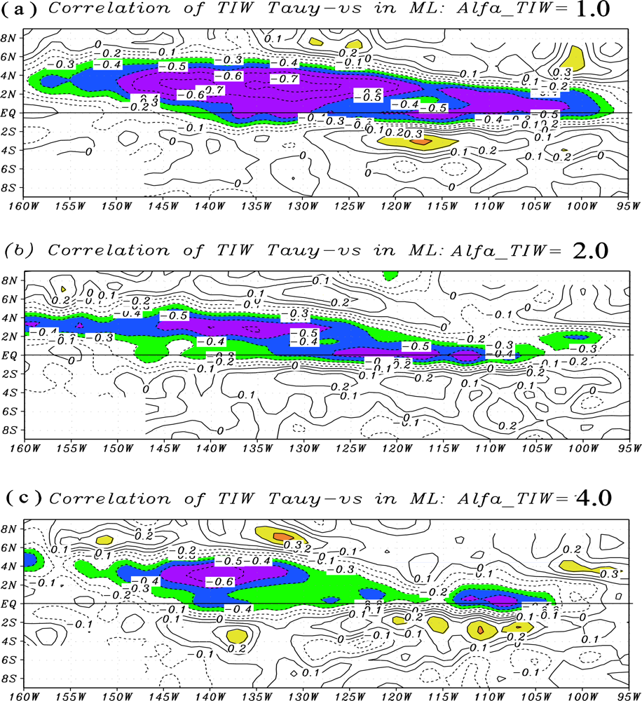
4.3. Relations between TIW-Scale Perturbations of Surface Atmospheric Winds and Oceanic Currents

Surface oceanic currents also exhibit coherent relationships with τTIW forcing at TIW scales in the feedback run. Following [21], we calculate the correlation coefficients between TIW-scale perturbations of surface currents (VTIW) and wind stress (τTIW), which is shown in Figure 11. It is seen that τ TIW y and V TIW y tends to be anti-correlated well over the eastern equatorial Pacific (Figure 11(b)). This indicates that surface currents in the ocean are directly affected by the TIW-scale wind. As demonstrated by [21], this anti-correlation is an indication of a negative feedback involved with the TIW-scale wind forcing, which acts to directly damp surface ocean currents, leading to a weakening of TIW activity in the ocean.

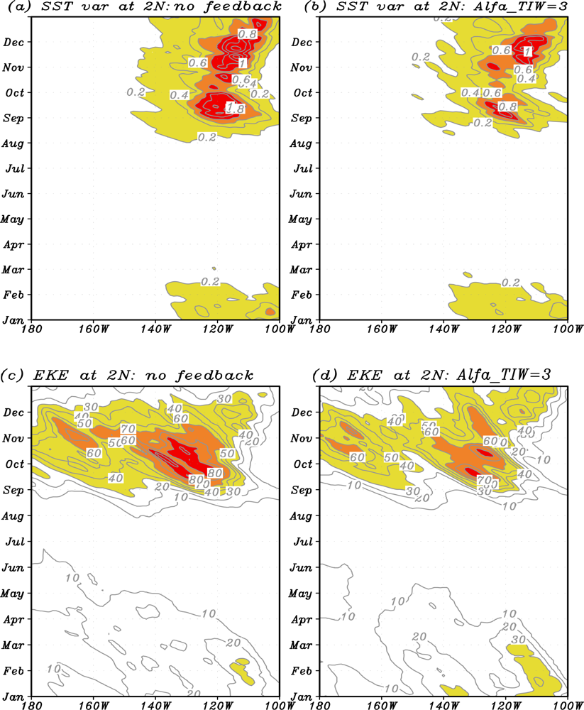
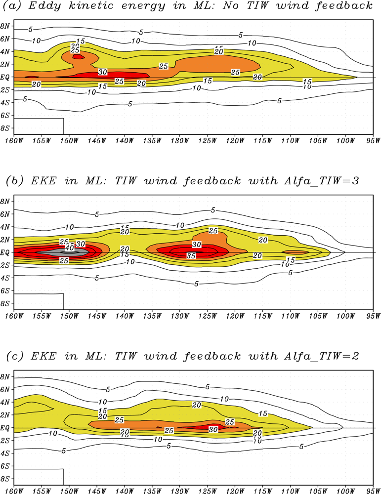
4.4. The Eddy Kinetic Energy (EKE)

Figures 6 and 7 show the spatial distribution of the sdv for EKE and its seasonal variation along the equatorial region, computed from the reference feedback run. The EKE has two maxima of over 35 kg·m−1·s−2, located respectively at 150°W and at 130°W–125°W on the equator. The regionally averaged EKE is about 21 kg·m−1·s−2 from 100°W to 160°W and from the equator to 5°N for the reference feedback run. It is worth noting that the EKE center tends to shift more to the equator in the feedback run.

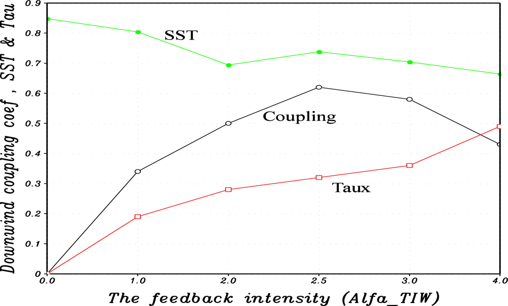
4.5. A Negative Feedback at TIW Scales

A comparison between the no-feedback run and the reference feedback run indicates clear differences in TIW activity in the ocean. In general, TIW variability becomes weaker in the feedback run compared with the no-feedback run. This can be visually seen not only in the SSTTIW fields, but also in other parameters representing TIW activity (Figures 4, 5, 6 and 7). For example, the weakening of TIWs is clearly seen in the sdv fields for SSTTIW (Figures 5 and 6). Quantitatively, in terms of the sdv for SSTTIW (Figure 5(a,b)), the amplitude of SSTTIW variability is reduced by about 17% in the feedback run relative to the no-feedback run. Note that the weakening of TIW activity in the feedback run is not well represented in the EKE field (Figure 7). In particular, the EKE even exhibits an increase in the regions from 130°W to 140°W on the equator in the feedback run compared with the no-feedback run, indicating that the effect of the TIW wind forcing on the EKE may be regionally dependent. Note that the EKE center shifts more to the equator when TIW wind feedback is explicitly included.
Associated with TIW wind effects, several negative feedbacks have been previously identified by [21,23]. In the no-feedback run in which τTIW is set to be zero, ocean currents are not influenced by TIW-scale surface winds. In the feedback run, a coherent anti-correlated pattern is seen between TIW-scale surface winds and currents (Figure 11), serving as a damping effect on TIWs in the ocean. These results are in line with other previous modeling studies, indicating that the surface wind-current coupling acts as a negative feedback onto TIW activity in the ocean. In addition, the apparent differences in the two runs indicate that TIW activity in the ocean and the related ocean-atmosphere coupling sensitively depends on the way TIW wind feedback is represented.

5. Discussion

As mentioned in the introduction, great uncertainties exist in representing TIW-induced wind feedback in global climate models. For example, many large-scale models currently used do not resolve TIW wind signals at all in the atmosphere; some underestimate them significantly, with TIW-induced wind feedback being underrepresented. We develop an empirical model for TIW-induced wind stress perturbations using satellite observations.
In the empirical representation of τTIW, its calculated amplitude and feedback effects on the ocean are dependent on the values of αTIW taken. As illustrated by [19], when αTIW varies, the τTIW amplitude is changed, but its structure is not. This scalar parameter can thus be used to serve as a way to represent the τTIW feedback intensity. The analyses from OGCM simulations using different values of αTIW can provide a quantification for the relationships between TIW-induced wind feedback intensity and its effects on the ocean. As demonstrated in [20], the effects on the large-scale ocean circulation in OGCM simulations of the tropical Pacific are characterized by a mean-state cooling of SST, with its cooling magnitude depending on the τTIW feedback intensity in a nonlinear way. For example, relative to the αTIW = 0.0 run, the maximum induced cooling effect occurs somewhere at around αTIW = 3.0. However, the effects on TIW activity in the ocean have not been examined in detail.
In this section, OGCM simulations with varying αTIW (Table 1) are analyzed to quantify the τTIW feedback effects on TIW activity in the ocean and the induced ocean-atmosphere coupling at TIW scales. The following specific questions are further discussed. How do the TIW activity and coupling vary as the τTIW feedback intensity changes? Are these relationships linear?

5.1. The τTIW and SSTTIW Fields

The τTIW feedback intensity derived using its empirical model (τTIW = αTIW·F(SSTTIW)) is determined by two factors, αTIW and SSTTIW. On one hand, a larger value of αTIW taken in the empirical calculation directly increases the amplitude of τTIW, leading to a stronger effect on the ocean. On the other hand, as demonstrated above, when allowing the ocean to be impacted interactively by τTIW, the TIW activity in the ocean tends to be dampened. As the SSTTIW variability is reduced, the τTIW response becomes weaker with decreased amplitude. Thus, an increase in αTIW can have two consequences in OGCM simulations with the induced TIW wind effects on the τTIW amplitude being opposite. This indicates that the way the τTIW feedback exerts an influence on TIW activity in the ocean and TIW-scale coupling can be sensitively dependent on its intensity (as represented by αTIW).
The relationships between τTIW feedback intensity and SSTTIW variability are further quantified in Table 1 when αTIW is taken to be varying (indicating different τTIW feedback intensity). A dampening effect on SSTTIW is seen in all the feedback runs compared with the no-feedback run. For example, as αTIW increases from 0.0 to 4.0, the τTIW amplitude increases monotonically (Table 1), and correspondingly TIWs in the ocean weaken with reduced SSTTIW variability.
Quantitatively, Figure 12 presents the spatial distributions of the sdv for τTIW and SSTTIW calculated from these feedback runs. Note that the reduction of SST variability is more notable in east (e.g., 110°W) when αTIW is increased, while there is much weaker change west of 125°W. In contrast, the sdv of τTIW is increased further west (e.g., 145°W). Thus, in the east, SST is strongly dampened by the coupling, and the consequent τTIW variability does not change much when αTIW is increased; but further west, SST is not dampened much and so τTIW variability increases significantly when αTIW is increased.
An inverse relationship between τTIW and SSTTIW is evident. A stronger τTIW feedback (a larger αTIW) tends to dampen SSTTIW more, which in turn acts to increase the response amplitude of τTIW, having stronger forcing effect on the ocean, with more dampening effects on SSTTIW variability. Also, it is seen that as αTIW increases from αTIW = 0.0 to αTIW = 4.0, the dampening effects on SSTTIW increase in a nonlinear way (Table 1). For example, when αTIW increases from αTIW = 1.0 to αTIW = 2.0, the sdv of τTIW increases by 47% from 0.019 dyn·cm−2 to 0.028 dyn·cm−2, and that of SSTTIW decreases by 14% from 0.402 °C to 0.347 °C; when αTIW increases from αTIW = 1.0 to αTIW = 3.0, the sdv of τTIW increases by 89%, and that of SSTTIW decreases by 12%. Clearly, these OGCM experiments indicate a negative feedback at TIW scales induced by TIW wind feedback in the ocean-atmosphere system.

5.2. TIW-Scale Coupling between the Ocean and Atmosphere

The ocean-atmosphere coupling at TIW scales is also a function of αTIW as shown in Table 1. Examples are further illustrated in Figure 13 for the feedback runs with αTIW = 1.0 and αTIW = 4.0, which can be compared with the corresponding reference feedback run with αTIW = 3.0 (Figure 8). Figure 14 illustrates the relationships between αTIW and the coupling parameters as represented by the wind stress divergence and downwind SST gradient (Table 1). It is clearly evident that TIW-scale coupling between the ocean and atmosphere depends on αTIW in a non-linear way. When taking αTIW = 0.0, τTIW is set to be zero and the TIW-scale coupling between the ocean and atmosphere is not allowed. At low values of αTIW in a weakly represented feedback regime (e.g., αTIW = 1.0 and αTIW = 2.0), TIW-scale coupling increases with αTIW. Interestingly, the TIW-scale coupling becomes decreased as αTIW increases above a threshold value. That is, at a certain value of αTIW, the coupling reaches a maximum; in these feedback runs performed using varying αTIW, the maximum coupling occurs somewhere at around αTIW = 2.5. As αTIW increases further to αTIW = 4.0 and larger, the TIW-scale coupling is reduced instead. This indicates that the coupling induced by TIW wind feedback can get saturated at certain intensity where a maximum TIW wind feedback effect is reached on the ocean.
Quantitatively, as represented by the TIW-scale divergence and downwind SST gradient fields in Table 1, the TIW-scale coupling coefficient is 0.4 in the αTIW = 1.0 run; it increases to 0.5 in the αTIW = 2.0 run and 0.62 in the αTIW = 2.5 run, but decreases to 0.6 in the αTIW = 3.0 run and to 0.43 in the αTIW = 4.0 run, respectively. Relative to the αTIW = 1.0 run, the TIW coupling increases by 47% in the αTIW = 2.0 run, by 82% in the αTIW = 2.5 run, and by 71% in the αTIW = 3.0 run.

5.3. The Correlations between TIW-Induced Wind Stress (τTIW) and Oceanic Currents (VTIW)

More examples for the correlations between τTIW and VTIW are shown in Figure 15 for different TIW wind feedback intensity represented. The level of the anti-correlation between τTIW and VTIW varies with αTIW. At αTIW = 1.0 the anti-correlation is the strongest; as αTIW increases, the level of the negative correlation becomes reduced. As analyzed by [21], these anti-correlations can serve as a negative feedback mechanism by which TIW-scale wind acts to damp TIW activity in the ocean.

6. Conclusion

TIWs are of oceanic origin, being modulated by many factors. For example, surface winds are a dominant one affecting TIW activity on seasonal and interannual time scales in the tropical Pacific. Additionally, TIW activity can be affected by TIW-scale wind forcing itself, as revealed by recent satellite observations and modeling studies. As SSTTIW is produced by TIWs in the ocean, TIW-scale wind perturbations are induced instantly in the atmosphere, which exert a direct influence back on TIW activity in the ocean. Furthermore, since TIWs are a major contributor to the mixed layer heat budget in the eastern tropical Pacific, a change in TIW activity can affect SSTs, a field that influences the weather and climate worldwide in association with ENSO [40,41]. In particular, as demonstrated in [20], SSTs are modulated by TIW-induced wind feedback through its effects on the horizontal advection and vertical mixing. Clearly, there exist close relationships among TIW activity in the ocean, TIW-scale coupling between the ocean and atmosphere, and SST in the eastern tropical Pacific. At present, these relationships are poorly understood and have not been quantified.
In our previous studies [19,30], remotely sensed data were used to derive a diagnostic model for TIW-induced wind stress perturbations (τTIW), which was embedded into an ocean general circulation model (OGCM). Without making use of a comprehensive TIW-resolving atmospheric model (which is computationally intensive), this embedded system allows to take into account a two-way coupling between the ocean and atmosphere at TIW scales in the eastern equatorial Pacific and further to represent the interactions between TIW-scale processes and the large scale ocean state. In this paper, the embedded system is used to examine the effects of TIW wind feedback on TIW activity in the ocean, with τTIW being interactively determined from TIW-scale sea surface temperature (SSTTIW) fields generated in the OGCM, written as τTIW = αTIW·F(SSTTIW). Sensitivity experiments with varying αTIW (representing TIW-scale wind feedback strength) are performed to illustrate a negative feedback induced by TIW-scale air–sea coupling and its relationship with TIW variability in the ocean. Consistent with previous modeling studies, TIW wind feedback tends to have a damping effect on TIWs in the ocean, with a general inverse relationship between the τTIW intensity and TIWs. Quantitatively, in terms of the standard deviation averaged in the region (0°N–5°N, 150°W–105°W), the SSTTIW amplitude is decreased by about 17% in the reference feedback run (αTIW = 3.0) relative to the no-feedback run. It is further shown that TIW-scale coupling does not vary linearly with αTIW: the coupling increases linearly with intensifying τTIW forcing at low values of αTIW (in a weak τTIW forcing regime); it becomes saturated at certain value of αTIW; it decreases when αTIW goes above a threshold value as the τTIW forcing increases further.
In this paper, the ocean-only experiments are performed to demonstrate the feasibility of using an empirical τTIW model to represent TIW wind feedback and the related TIW-scale coupling, and their interactions with large-scale ocean circulation. Together with the demonstrated effect on the mean ocean state presented in [20], TIW wind feedback is seen to exert a noticeable influence on the mean ocean state (e.g., SST), TIW activity in the ocean, and TIW-scale coupling between the ocean and atmosphere in the tropical Pacific. It is thus necessary to adequately take into account TIW-scale feedback effects in large-scale climate modeling. As realistic representations of TIW-scale wind responses are still a great challenge in large-scale climate models, the empirical modeling approach tested in this paper offers a simple and an effective way to parameterize TIW-induced wind forcing. Needless to say that the mechanistic understanding of TIW wind feedback and its empirical parameterization presented in this paper can be transferred to more realistic coupled climate models to enhance our predictive understanding of the TIW wind feedback effects in the tropical Pacific, benefiting to ENSO prediction [41].
An innovative aspect of this work is to utilize satellite observations (SST and ocean vector wind) to improve parameterizations of TIW wind feedback effects that are still missing in many large-scale climate models. Previously, a similar approach has been taken to use Topex/Poseidon-Jason sea level data to improve representations of the subsurface ocean entrainment temperature (Te) for use in ocean and coupled ocean-atmosphere models [42], to use satellite ocean color data to represent ocean biology-induced climate feedback [36,43], to use satellite precipitation data to represent freshwater flux-induced climate feedback [37], and to use satellite wind data to represent tropical cyclone wind-induced forcing effect [44], respectively. Taking these together, we demonstrate new and comprehensive ways to make full use of satellite data to represent, not only physical, but also biological processes for ocean and climate modeling in the tropical Pacific.

Acknowledgments

We would like to thank A.J. Busalacchi, W.S. Kessler, D. Chelton, S.-P. Xie and C. Menkes for their comments. The authors wish to thank anonymous reviewers for their numerous comments. We appreciate helps from E. Hackert and R.F. Milliff for the QuikSCAT wind data. The TMI SST data are directly downloaded from the Remote Sensing Systems website at www.remss.com. This research is supported in part by NSF Grant (ATM-0727668), NOAA Grant (NA08OAR4310885) and NASA Grants (NNX08AI74G, NNX08AI76G and NNX09AF41G); Li and Min are supported by Meteorology Commonweal Special Project of Science and Technology of People’s Republic of China (GYHY200806029) and by “The Priority Academic Program Development (PAPD) of Jiangsu Higher Education Institutions”.
  • Conflict of InterestThe authors declare no conflict of interest.

References

  1. Legeckis, R. Long waves in the eastern equatorial Pacific Ocean: A view from a geostationary satellite. Science 1977, 197, 1179–1181. [Google Scholar]
  2. Bryden, H.L.; Brady, E.C. Eddy momentum and heat fluxes and their effects on the circulation of the equatorial Pacific Ocean. J. Mar. Res 1989, 47, 55–79. [Google Scholar]
  3. Wallace, J.M.; Mitchell, T.P.; Deser, C. The influence of sea surface temperature on surface wind in the eastern equatorial Pacific: Seasonal and interannual variability. J. Clim 1989, 2, 1492–1499. [Google Scholar]
  4. Baturin, N.; Niiler, P. Effects of instability waves in the mixed layer of the equatorial Pacific. J. Geophys. Res 1997, 102, 27771–27793. [Google Scholar]
  5. Qiao, L.; Weisberg, R.H. Tropical instability wave energetics: Observations from the tropical instability wave experiment. J. Phys. Oceanogr 1998, 28, 345–360. [Google Scholar]
  6. Masina, S.; Philander, S.G.H. An analysis of tropical instability waves in a numerical model of the Pacific Ocean. I. Spatial variability of the waves. J. Geophys. Res 1999, 104, 29613–29635. [Google Scholar]
  7. Kessler, W.S.; Rothstein, L.M.; Chen, D. The annual cycle of SST in the eastern tropical Pacific, diagnosed in an ocean GCM. J. Clim 1998, 11, 777–799. [Google Scholar]
  8. Kessler, W.S.; Kleeman, R. Rectification of the Madden–Julian Oscillation into the ENSO cycle. J. Clim 2000, 13, 3560–3575. [Google Scholar]
  9. Jochum, M.; Cronin, M.F.; Kessler, W.S.; Shea, D. Observed horizontal temperature advection by tropical instability waves. Geophys. Res. Lett 2007, 34, L09604. [Google Scholar]
  10. Jochum, M.; Deser, C.; Phillips, A. Tropical atmospheric variability forced by oceanic internal variability. J. Clim 2007, 20, 765–771. [Google Scholar]
  11. Chelton, D.B.; Esbensen, S.K.; Schlax, M.G.; Thum, N.; Freilich, M.H.; Wentz, F.J.; Gentemann, C.L.; McPhaden, M.J.; Schopf, P.S. Observations of coupling between surface wind stress and sea surface temperature in the eastern tropical Pacific. J. Clim 2001, 14, 1479–1498. [Google Scholar]
  12. Xie, S.-P. Satellite observations of cool ocean-atmosphere interaction. Bull. Amer. Meteor. Soc 2004, 85, 195–208. [Google Scholar]
  13. Lee, T.; Lagerloef, G.; Gierach, M.M.; Kao, H.-Y.; Yueh, S.S.; Dohan, K. Aquarius reveals salinity structure of tropical instability waves. Geophys. Res. Lett 2012, 39, L12610. [Google Scholar]
  14. Wentz, F.J.; Gentemann, C.; Smith, D.; Chelton, D. Satellite measurements of sea surface temperature through clouds. Science 2000, 288, 847–850. [Google Scholar]
  15. Kravtsov, S.; Kondrashov, D.; Kamenkovich, I.; Ghil, M. An empirical stochastic model of sea-surface temperatures and surface winds over the Southern Ocean. Ocean Sci 2012, 7, 755–770. [Google Scholar]
  16. Liu, W.T.; Xie, X.; Polito, P.S.; Xie, S.-P.; Hashizume, H. Atmospheric manifestation of tropical instability waves observed by QuikSCAT and Tropical Rain Measuring Mission. Geophys. Res. Lett 2000, 27, 2545–2548. [Google Scholar]
  17. Chelton, D.B.; Schlax, M.G.; Freilich, M.H.; Milliff, R.F. Satellite measurements reveal persistent small-scale features in ocean winds. Science 2004, 303, 978–983. [Google Scholar]
  18. Hashizume, H.; Xie, S.-P.; Liu, W.T.; Takeuchi, K. Local and remote atmospheric response to tropical instability waves: A global view from the space. J. Geophys. Res 2001, 106, 10173–10185. [Google Scholar]
  19. Zhang, R.-H.; Busalacchi, A.J. An empirical model for surface wind stress response to SST forcing induced by tropical instability waves (TIWs) in the eastern equatorial Pacific. Mon. Wea. Rev 2009, 137, 2021–2046. [Google Scholar]
  20. Zhang, R.-H. Effects of tropical instability wave (TIW)-induced surface wind feedback. Clim. Dyn. 2013, in press.. [Google Scholar]
  21. Seo, H.; Jochum, M.; Murtugudde, R.; Miller, A.J.; Roads, J.O. Feedback of tropical instability-wave-induced atmospheric variability onto the ocean. J. Clim 2007, 20, 5842–5855. [Google Scholar]
  22. Pezzi, L.P.; Vialard, J.; Richards, K.J.; Menkes, C.; Anderson, D. Influence of ocean-atmosphere coupling on the properties of tropical instability waves. Geophys. Res. Lett 2004, 31, L16306. [Google Scholar]
  23. Small, R.J.; Richards, K.J.; Xie, S.-P.; Dutrieux, P.; Miyama, T. Damping of tropical instability waves caused by the action of surface currents on stress. J. Geophys. Res 2009, 114, C04009. [Google Scholar]
  24. Lien, R.-C.; D’Asaro, E.A.; Menkes, C.E. Modulation of equatorial turbulence by tropical instability waves. Geophys. Res. Lett 2008, 35, L24607. [Google Scholar]
  25. Moum, J.N.; Lien, R.-C.; Perlin, A.; Nash, J.D.; Gregg, M.C.; Wiles, P.J. Sea surface cooling at the Equator by subsurface mixing in tropical instability waves. Nat. Geosci 2009, 2, 761–765. [Google Scholar]
  26. Contreras, R.F. Long-term observations of tropical instability waves. J. Phys. Oceanogr 2002, 32, 2715–2722. [Google Scholar]
  27. Xie, S.-P.; Miyama, T.; Wang, Y.; Xu, H.; de Szoeke, S.P.; Small, R.J.; Richards, K.J.; Mochizuki, T.; Awaji, T. A regional ocean–atmosphere model for eastern Pacific climate: Toward reducing Tropical biases. J. Clim 2006, 20, 1504–1522. [Google Scholar]
  28. Roberts, M.J.; Clayton, A.; Demory, M.-E.; Donners, J.; Vidale, P. L.; Norton, W.; Shaffrey, L.; Stevens, D.P.; Stevens, I.; Wood, R.A.; et al. Impact of resolution on the tropical Pacific circulation in a matrix of coupled models. J. Clim 2009, 22, 2541–2556. [Google Scholar]
  29. Shaffrey, L.C.; Stevens, I.; Norton, W.A.; Roberts, M.J.; Vidale, P.L.; Harle, J.D.; Jrrar, A.; Stevens, D.P.; Woodage, M.J.; Demory, M.E.; et al. UK HiGEM: The new UK high-resolution global environment model—Model description and basic evaluation. J. Clim 2009, 22, 1861–1896. [Google Scholar]
  30. Zhang, R.-H.; Busalacchi, A.J. Rectified effects of tropical instability wave (TIW)-induced atmospheric wind feedback in the tropical Pacific. Geophys. Res. Lett 2008, 35, L05608. [Google Scholar]
  31. Gent, P.; Cane, M.A. A reduced gravity, primitive equation model of the upper equatorial ocean. J. Comp. Phys 1989, 81, 444–480. [Google Scholar]
  32. Chen, D.; Rothstein, L.M.; Busalacchi, A.J. A hybrid vertical mixing scheme and its application to tropical ocean models. J. Phys. Oceanogr 1994, 24, 2156–2179. [Google Scholar]
  33. Murtugudde, R.; Seager, R.; Busalacchi, A.J. Simulation of tropical oceans with an ocean GCM coupled to an atmospheric mixed layer model. J. Clim 1996, 9, 1795–1815. [Google Scholar]
  34. Murtugudde, R.; Beauchamp, J.; McClain, C.R.; Lewis, M.; Busalacchi, A.J. Effects of penetrative radiation on the upper tropical ocean circulation. J. Clim 2002, 15, 470–486. [Google Scholar]
  35. Zhang, R.-H.; Busalacchi, A.J.; Murtugudde, R.G. Improving SST anomaly simulations in a layer ocean model with an embedded entrainment temperature submodel. J. Clim 2006, 19, 4638–4663. [Google Scholar]
  36. Zhang, R.-H.; Busalacchi, A.J.; Wang, X.; Ballabrera-Poy, J.; Murtugudde, R.G.; Hackert, E.C.; Chen, D. Role of ocean biology-induced climate feedback in the modulation of El Niño-Southern Oscillation. Geophys. Res. Lett 2009, 36, L03608. [Google Scholar]
  37. Zhang, R.-H.; Zheng, F.; Zhu, J.; Pei, Y.; Zheng, Q.; Wang, Z. Modulation of El Niño-southern oscillation by freshwater flux and salinity variability in the tropical Pacific. Adv. Atmos. Sci 2012, 29, 647–660. [Google Scholar]
  38. O’Neill, L.W.; Chelton, D.B.; Esbensen, S.K. The effects of SST-induced surface wind speed and direction gradients on midlatitude surface vorticity and divergence. J. Clim 2010, 23, 255–281. [Google Scholar]
  39. Chelton, D.B. The impact of SST specification on ECMWF surface wind stress fields in the eastern tropical Pacific. J. Clim 2005, 18, 530–550. [Google Scholar]
  40. Zhang, R.-H.; Levitus, S. Interannual variability of the coupled Tropical Pacific ocean-atmosphere system associated with the El Nino/Southern Oscillation. J. Clim 1997, 10, 1312–1330. [Google Scholar]
  41. Zhang, R.-H.; Zheng, F.; Zhu, J.; Wang, Z.G. A successful real-time forecast of the 2010–11 La Niña event. Sci. Rep. 2013. [Google Scholar] [CrossRef]
  42. Zhang, R.-H.; Busalacchi, A.J.; Murtugudde, R.G.; Hackert, E.C.; Ballabrera-Poy, J. A new approach to improved SST anomaly simulations using altimeter data: Parameterizing entrainment temperature from sea level. Geophys. Res. Lett 2004, 31, L10304. [Google Scholar]
  43. Zhang, R.-H.; Chen, D.; Wang, G. Using satellite ocean color data to derive an empirical model for the penetration depth of solar radiation (Hp) in the tropical Pacific ocean. J. Atmos. Ocean. Technol 2011, 28, 944–965. [Google Scholar]
  44. Zhang, R.-H.; Pei, Y.; Chen, D. Remote effects of tropical cyclone (TC) wind forcing over the western Pacific on the eastern equatorial ocean. Adv. Atmos. Sci. 2013, in press.. [Google Scholar]
Figure 1. A schematic diagram showing the use of satellite data to represent Tropical Instability Waves (TIW)-induced surface wind feedback in a basin-scale ocean general circulation model (OGCM) of the tropical Pacific. The OGCM is forced by a prescribed climatological wind stress (τclim) field and TIW-scale surface wind stress field (τTIW) over the central-eastern tropical Pacific, with the latter (τTIW) being derived using an empirical model constructed from satellite observations, written as τTIW = αTIW·F(SSTTIW). Then, given a TIW-scale SST perturbation (SSTTIW) from the OGCM, τTIW is determined accordingly. The derived τTIW part can be taken into account or not for ocean modeling, allowing isolation of its feedback effect on the ocean in a clean way.
Remotesensing 05 02660f1
Figure 2. Horizontal distributions of (a) total sea surface temperatures (SSTs) and (b) the zonal-high-pass filtered SST fields (SSTTIW) on 1 October 1999 from the satellite data, and of the TIW-induced (c) zonal and (d) meridional wind stress components on 1 October 1999, simulated from the SSTTIW fields in (b) using the empirical τTIW model with αTIW = 1 taken and the first 10 singular vector decomposition (SVD) modes retained. The contour interval is 1 °C in (a), and 0.3 °C in (b), and 0.03 dyn·cm−2 in (c,d).
Remotesensing 05 02660f2
Figure 3. Spatial patterns of the first pair of eigenvectors for (a) SSTTIW, and for (b) zonal and (c) meridional τTIW components, respectively. The SVD analysis is performed using the TMI SST and QuikSCAT wind satellite data during the periods 2000–2007. The contour interval is 0.3 in (a) and 0.1 in (b,c).
Remotesensing 05 02660f3
Figure 4. Longitude-time sections of the zonal-high-pass filtered fields along 2°N during July-December calculated from the ocean general circulation model (OGCM) simulations in year 13: the SSTTIW fields obtained from (a) the no-feedback run and (b) the feedback run, and the (c) zonal and (d) meridional τTIW fields derived from the SSTTIW field shown in (b) using the empirical τTIW model with αTIW = 3.0 and the first 10 SVD modes retained. The contour interval is 0.3 °C in (a,b), and is 0.02 dyn·cm−2 in (c,d).
Remotesensing 05 02660f4
Figure 5. Horizontal distributions for the standard deviation (sdv) of SSTTIW calculated from (a) the no-feedback run and from the TIW wind feedback runs with (b) αTIW = 3.0 and (c) αTIW = 2.0, respectively. The calculations are made from daily SSTTIW data in year 13. The contour interval is 0.1 °C.
Remotesensing 05 02660f5
Figure 6. Seasonal variations along 2°N for the sdv of SSTTIW (upper panels) and of the eddy kinetic energy (EKE) (low panels) calculated from the OGCM simulations (left panels) without and (right panels) with the TIW wind feedback, respectively. The calculations are made from daily SST and surface mixed-layer current data in year 13. The contour interval is 0.2 °C in (a,b), and is 10 kg·m−1·s−2 in (c,d).
Remotesensing 05 02660f6
Figure 7. Horizontal distributions of the EKE calculated (a) from the no-feedback run and from the feedback runs with (b) αTIW = 3.0 and (c) αTIW = 2.0, respectively. The calculations are made from the zonal-high-pass filtered current fields in year 13. The contour interval is 5 kg·m−1·s−2.
Remotesensing 05 02660f7
Figure 8. Time-longitude sections during August-December in the reference feedback run (αTIW = 3.0 taken and the first 10 SVD modes retained): (a) the zonal-high-pass filtered downwind component of the SST gradient along 2°N and (b) the corresponding wind stress divergence; (c) the zonal-high-pass filtered crosswind component of the SST gradient along 0.5°N and (d) the corresponding wind stress curl. The calculations are made from daily SST and τTIW fields in year 13. The contour is 0.3 °C per 100 km in (a,c), and is 0.3 N·m−2 per 104 km in (b,d).
Remotesensing 05 02660f8
Figure 9. Examples of the horizontal patterns on 1 October, calculated from the reference feedback run: (a) the downwind component of the SST gradient; (b) the wind stress divergence; (c) the crosswind component of the SST gradient; and (d) the wind stress curl, respectively. The contour is 0.2 °C per 100 km in (a,c), and is 0.2 N·m−2 per 104 km in (b,d).
Remotesensing 05 02660f9
Figure 10. Binned scatterplots of the relationship between the zonal-high-pass filtered wind stress divergence and downwind component of the SST gradient (the black line with open circles), and the zonal-high-pass filtered wind stress curl and crosswind component of the SST gradient (the red line with close circles), which are computed over the region (0°N −5°N, 150°W −105°W) during the cold season (August–December). The y-axis unit is N·m−2 per 104 km and the x-axis unit is °C per 100 km, respectively.
Remotesensing 05 02660f10
Figure 11. Horizontal distributions of the correlations between the high-pass-filtered wind stress and surface-layer current fields for their (a) zonal and (b) meridional components, computed using daily data in year 13 from the reference feedback run. The contour interval is 0.1.
Remotesensing 05 02660f11
Figure 12. Zonal distributions along 2°N for the sdv of (a) the zonal τTIW and (b) SSTTIW fields, calculated using daily data in year 13. The results are given for the feedback runs with αTIW = 3.0 (the line with open circles), αTIW = 1.0 (the line with open squares), αTIW = 2.0 (the line with full circles), and αTIW = 4.0 (the line with full squares), respectively. Also given in (b) is the sdv of SSTTIW calculated from the no-feedback run (the line with plus symbols). The unit is dyn·cm−2 in (a) and °C in (b).
Remotesensing 05 02660f12
Figure 13. Time-longitude sections along 2°N during August-December for the (left panels) zonal-high-pass filtered downwind component of the SST gradient, and (right panels) wind stress divergence, estimated from the feedback runs with αTIW = 1.0 ((a,b)) and αTIW = 4.0 ((c,d)), respectively. The calculations are made from daily SST data in year 13. The contour is 0.3 °C per 100 km in (a,c), and is 0.3 N·m−2 per 104 km in (b,d).
Remotesensing 05 02660f13aRemotesensing 05 02660f13b
Figure 14. Variations in the TIW coupling coefficient, and the sdv of the zonal τTIW component and of SSTTIW fields, which are expressed as a function of TIW wind feedback intensity (represented by αTIW). The TIW-scale coupling is represented by the binned slopes between the zonal-high-pass filtered wind stress divergence and the downwind component of the SST gradient, whose computations are made using daily data over the region (0°N–5°N, 150°W–105°W) during the cold season (August–December) in year 13. The unit is N·m−2 per 104 km for the coupling coefficient; to use the same y-axis for indicating the units of τTIW and of SSTTIW, the sdv values for τTIW and of SSTTIW plotted in the figure are multiplied respectively by 10 and 2, respectively.
Remotesensing 05 02660f14
Figure 15. Horizontal distributions of the correlations between the high-pass-filtered meridional wind stress and surface-layer current fields in some additional feedback runs, with (a) αTIW = 1.0; (b) αTIW = 2.0; and (c) αTIW = 4.0, respectively. The calculations are made using daily data in year 13. The contour interval is 0.1.
Remotesensing 05 02660f15
Table 1. The spatially averaged sdv for the zonal τTIW and SSTTIW fields in the region (0°N–5°N, 150°W–105°W), calculated using daily data in year 13. Also given are the binned slopes between the zonal-high-pass filtered wind stress divergence and the downwind component of the SST gradient (Downwind coupling coefficient), and between the zonal-high-pass filtered wind stress curl and the crosswind component of the SST gradient (Crosswind coupling coefficient), whose computations are made over the region (0°N–5°N, 150°W–105°W) during the cold season (August–December). Results are shown as a function of TIW wind feedback intensity, indicated by the rescaling factor, αTIW, ranging from αTIW = 0.0 (no TIW wind) to αTIW = 4.0 (a strong TIW wind case), respectively. The unit is dyn·cm−2 for τTIW, °C for SSTTIW, and is N·m−2 per 104 km for the coupling coefficients.
αTIWSdv of τTIWSdv of SSTTIWDownwind Coupling CoefCorsswind Coupling Coef
0.00.00.4240.00.0
1.00.0190.4020.340.14
2.00.0280.3470.500.22
2.50.0320.3690.620.24
3.00.0360.3520.580.25
4.00.0490.3320.430.17

