Article

Early Detection of Bark Beetle Green Attack Using TerraSAR-X and RapidEye Data

by
Sonia M. Ortiz
1,*,
Johannes Breidenbach
2 and
Gerald Kändler
1
1
Department of Biometrics, Forest Research Institute of Baden-Württemberg, Wonnhaldestr. 4, D-79100 Freiburg, Germany
2
Norwegian Forest and Landscape Institute, Postboks 115, N-1431 Ås, Norway
*
Author to whom correspondence should be addressed.
Remote Sens. 2013, 5(4), 1912-1931; https://doi.org/10.3390/rs5041912
Submission received: 18 February 2013 / Revised: 4 April 2013 / Accepted: 4 April 2013 / Published: 16 April 2013

Abstract

:
Bark beetles cause widespread damages in the coniferous-dominated forests of central Europe and North America. In the future, areas affected by bark beetles may further increase due to climate change. However, the early detection of the bark beetle green attack can guide management decisions to prevent larger damages. For this reason, a field-based bark beetle monitoring program is currently implemented in Germany. The combination of remote sensing and field data may help minimizing the reaction time and reducing costs of monitoring programs covering large forested areas.
In this case study, RapidEye and TerraSAR-X data were analyzed separately and in combination to detect bark beetle green attack. The remote sensing data were acquired in May 2009 for a study site in south-west Germany. In order to distinguish healthy areas and areas affected by bark beetle green attack, three statistical approaches were compared: generalized linear models (GLM), maximum entropy (ME) and random forest (RF). The spatial scale (minimum mapping unit) was 78.5 m2.
TerraSAR-X data resulted in fair classification accuracy with a cross-validated Cohen’s Kappa Coefficient (kappa) of 0.23. RapidEye data resulted in moderate classification accuracy with a kappa of 0.51. The highest classification accuracy was obtained by combining the TerraSAR-X and RapidEye data, resulting in a kappa of 0.74. The accuracy of ME models was considerably higher than the accuracy of GLM and RF models.

1. Introduction

In central Europe, climate change has been predicted to increase annual mean temperatures and cause more frequent extreme weather events. These effects are known for promoting forest diseases [1]. Salvage cuttings of trees affected by bark beetles (Ips typographus L.) resulted in considerable amounts of unplanned harvests in recent years in Germany [2]. Therefore, a terrestrial bark beetle monitoring program is implemented by the forest service in areas dominated by Norway spruce. However, new bark beetle spots are hard to identify and the surveys are time consuming and expensive.
By combining high resolution satellite imagery with terrestrial data, it may be possible to minimize the response time and reduce costs involved in the monitoring of large forested areas. Optical sensors (passive remote sensing systems) have proved to be useful for this purpose as they can detect changes in forest health over time especially using near-infrared channels [3]. The disadvantage of passive systems is that they are more affected by weather conditions than active systems. Active systems, such as synthetic aperture radar (SAR), are an alternative in regions where cloud cover complicates the acquisition of optical data [4]. Another advantage of SAR systems, in comparison with optical data, is the capability to penetrate the forest canopy to some degree. Since microwave and optical data offer complementary information that can improve the classification accuracy [5], the combination of SAR and optical data has become an important focus of remote sensing research [6].
The capabilities of optical satellite data to detect the first stage of a bark beetle infestation, known as the green attack, are limited because no discoloration of the needles occurs at this stage [3]. However, recently launched optical satellites include the red-edge band that allows the identification of changes in the health of green vegetation in early phases [7,8]. The green attack is followed by red attack in which the identification of infested trees is easier due to the discoloration of the foliage in the visual spectrum [9].
Murtha and Wiart [10] analyzed color-infrared aerial photographs to detect differences between lodgepole pine with and without bark beetle green attack in Canada. Although they observed spectral differences in the green and red channels, overlaps between the two classes did not allow to accurately distinguish between the infested and healthy trees. Heath [11] encountered similar challenges by using airborne multispectral data. In contrast, Roberts et al.[12] reported high accuracy for the early detection of bark beetle green attack in late May and early June with multispectral images. Schweigler [13] identified single Norway spruce trees with green attack in south-west Germany using visible bands of aerial panoramic photos. Marx [14] used multitemporal RapidEye data for the detection of forest stands with bark beetle green and red attack in eastern Germany. By means of supervised classification, red attack was identified with high accuracy. The identification of green attack was less satisfactory due to small differences in the spectral response between healthy and attacked trees. Eitel et al.[7] also used RapidEye data to analyze the capabilities of the red-edge band for early detection of stress induced by girdling of conifers in New Mexico. They concluded that RapidEye data may be useful for detecting bark beetle green attack.
SAR data have been frequently used for the detection and quantification of forest disturbances [4]. Recently, Tanase et al.[15,16] analyzed TerraSAR-X images to map burned Mediterranean forest. Solberg et al.[17] evaluated TerraSAR-X data for monitoring pine sawfly damages in boreal forest, observing that backscatter intensity and coherence were sensitive to leaf area index variations. In addition, Ackermann and Klaus [18] reported that TerraSAR-X data was suitable for mapping pine sawfly defoliation in Germany.
Trees infested by bark beetles tend to have a lower tissue moisture content compared to non-infested trees [19,20]. Considering the relationship between radar backscatter and the dielectric constant of tree tissues [21], it may be expected that TerraSAR-X imagery can be used for identifying trees infested by bark beetles. Healthy trees should result in a higher SAR backscatter than dry (infested) or dead trees [22]. However, the accuracy of the image classification depends not only on the remote sensing data, but also on the classification method [23]. Furthermore, in the case of supervised classification, the accuracy also depends on the type, number and quality of the reference data [24,25]. The number of ground observations of bark beetle green attack at endemic levels will often be limited, which highlights the importance of using statistical methods that can handle small sample sets.
This study aimed on evaluating the capabilities of RapidEye and TerraSAR-X imagery for detecting of areas affected by bark beetle green attack. An early detection of bark beetle (Ips typographus L.) green attack may guide management actions to prevent larger damages. RapidEye and TerraSAR-X imagery were evaluated separately and in combination. Three statistical approaches were compared: (a) generalized linear models (GLM), (b) maximum entropy (ME), and (c) random forest (RF). The principal difference between the approaches is that GLM and RF are suited for modelling more or less balanced presence-absence data, while ME is capable of handling presence-only data [26]. The three methods were selected with the aim of evaluating parametric, semiparametric and non-parametric approaches.

2. Material and Methods

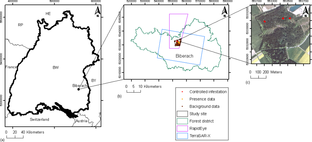
2.1. Study Site and Field Data

The study site is located in the forest district of Biberach (Figure 1) in south-west Germany (48°8′N, 9°43′E). The study site was given by the overlap area of TerraSAR-X and RapidEye images (see Section 2.2) as well as spruce-dominated forest (Figure 1(b), black polygon). The topography is flat with elevations between 500 m and 650 m above sea level. The forest in the study site is dominated by Norway spruce (Picea abies (L.) Karst.), which covered 71% of the area. Other tree species included beech (Fagus sylvatica L.) (14%) and oak (Quercus rubra and Quercus petrea (Liebl.)) (5%). The remaining 10% of the forest is covered by almost equal amounts of Douglas-fir (Pseudotsuga menziesii (Mirb.) Franco), ash (Fraxinus excelsior), Scots pine (Pinus sylvestris L.), silver fir (Abies alba Mill), and European larch (Larix decidua). The age of the forest stands ranged between 10 and 100 years and tree heights varied between 10 m and 35 m [27].
To ensure presence of trees with bark beetle green attack at the study site, three groups of eight trees were chosen to promote a bark beetle infestation with pheromone dispensers. The tree groups were located in a forest area that was separated from other forests by other land uses (Figure 1(c)). The positions of the tree groups were determined by entomologists of the Forest Research Institute of Baden-Württemberg (FVA). The groups had to be as far away from interior edges as possible, but in areas with enough sunlight to ensure an adequate temperature for the development of the bark beetles. The pheromone dispensers were mounted on the 3 April 2009 and the tree groups were monitored once a week until 18 September 2009. This survey was conducted independently of the conventional monitoring of the forest service. Differentially corrected Global Positioning System (DGPS) coordinates were collected for all trees with symptoms of a bark beetle infestation in the area. A total of 28 trees with symptoms of bark beetle attack were identified in the field in May 2009 when the remote sensing data were acquired. The visual discoloration of the foliage began mid-June 2009. Thirteen of the trees survived the bark beetle infestation while 15 trees died between July and September 2009.
In parallel, the forest service carried out the conventional terrestrial monitoring of bark beetle attack in the entire forest district (Figure 1(b), green polygon). The approximate location of the detected trees with symptoms was marked on maps with a scale of 1:10,000 to guide harvesting teams to the trees. These maps were used to obtain additional reference data for the study. DGPS coordinates with an approximate positioning accuracy of 3 m were collected for the marked locations on the maps with more than two infested neighboring trees. Trees infested by bark beetles located close to forest gaps or forest borders were omitted to avoid edge effects. A total of nine references (each comprising of three or more trees) with DGPS coordinates were included to the sample data set for modeling (Figure 1(b), yellow points).

2.2. Satellite Data

RapidEye and TerraSAR-X images with one day time difference between the acquisitions were provided by the German Aerospace Centre (DLR) in May 2009 (Table 1). The RapidEye image was a systematically geocorrected L2A radiance product [28]. The image was radiometrically, sensor, and geometrically corrected and aligned in UTM map projection by the data provider. The geometric correction was carried out using a coarse digital elevation model (DEM) of the Shuttle Radar Topography Mission (SRTM) without the incorporation of ground control points [28]. The image originally had a ground resolution of 6.5 m but was resampled to 5 m during orthorectification. The atmosphere was free of clouds during acquisition. However, only 41% of the scene contained data (Figure 1).
The TerraSAR-X image was acquired in StripMap (SM) mode with HH polarization. In the SM mode, the ground swath was illuminated with a continuous sequence of pulses with the antenna beam fixed in elevation and azimuth [29]. The image was provided as a Single Look Slant Range Complex (SSC) product [30].

2.2.1. Pre-Processing of RapidEye Data

A visual comparison indicated a shift of the RapidEye image in relation to the orthorectified SAR image. This systematic error is known for Level 2A products [31]. Since the SAR image was orthorectified using a highly accurate digital surface model (DSM), the position of the RapidEye image was rectified using the orthorectified TerraSAR-X image as a reference.
The next pre-processing step was to convert the radiance values to top of atmosphere reflectance (TOA) [28]. In contrast to the radiance, the reflectance can be considered as a property of the material being observed that is not dependent on the illumination, orientation and position of the target. Reflectance images are generally more suitable than radiance images to calculate vegetation indices [32].
Band ratios and several vegetation indices were calculated for each pixel (see Table 2 for all indices).

2.2.2. Pre-Processing of TerraSAR-X Data

An absolute calibration of the backscattered complex signal was carried out for the SSC product by applying the constant factor (k) delivered with the data. This is equivalent to computing the radar brightness (β0) that represents the radar reflectivity per unit area in slant range:
β 0 = k ( i 2 + q 2 ) 2
where i and q represent the imaginary and real parts of the digital numbers in the image [33].
To reduce errors in the pixel location, the β0 image was orthorectified using a high resolution digital surface model (DSM) with a resolution of 2 m derived from airborne laser scanning (ALS) first returns. The ALS data were collected in the winter of 2002 by the Land Survey Bureau of Baden-Württemberg (LGL) and have an approximate density of 0.5 points per square meter [34]. The DSM was computed using the software TreesVis [35].
The orthorectification was based on a look-up table containing the transformation between the radar and the map geometry [36] implemented in the software GAMMA [37]. The look-up table was derived from orbital information and elevation of the DSM, and was refined for increased precision by estimating offsets between the SAR image and a simulated SAR image derived from the DSM as reference. The SAR image was finally transformed to map geometry using the refined look-up table. The map projection of the orthorectified image with 2 m pixel size was UTM zone 32N.
To correct the effects of the incidence angle on the pixel values, the SAR data was radiometrically calibrated by calculating the radar reflectivity per unit area in ground range (σ0):
σ 0 = β 0 sin ( Θ loc )
where σ0 represents the scattering coefficient, β0 constitutes the radar brightness and Θloc is the local incidence angle [33].

2.3. Statistical Modelling

Our aim was to identify parsimonious models that adequately explained the data. Three statistical approaches (ME, GLM and RF) were compared. Explanatory variables calculated from RapidEye and TerraSAR-X imagery were evaluated separately and in combination. The calculation of the explanatory variables and the statistical approaches is described in the following subsections.

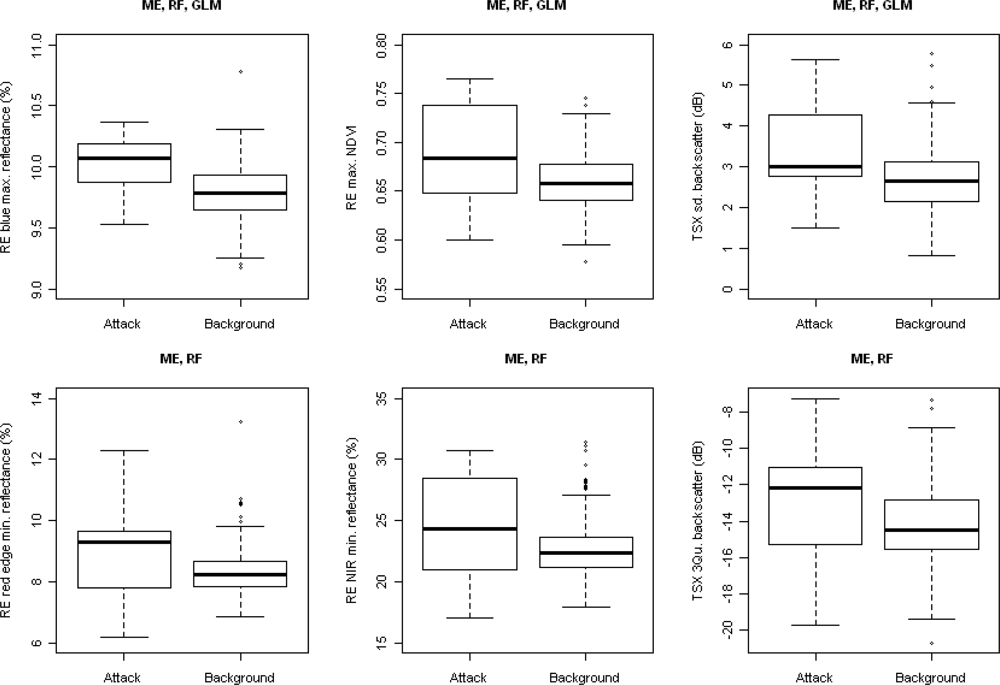
2.3.1. Explanatory Variables

To link remote sensing and field data, circular plots, each with 5 m radius, were created to cover groups of three or more trees with bark beetle green attack observed in the field. The midpoints of the plots were the center coordinates of the tree positions. The radius of 5 m was chosen in order to consider the average crown diameter (5 m to 6 m) of the trees and the approximate positioning error of the DGPS coordinates (up to 3 m). The overlap of neighboring plots was in no case larger than 10%. Furthermore, plots had to be located more than 10 m away from forest borders. A total of 15 plots were used as references for the bark beetle green attack (presence data) to fit the statistical models.
To obtain data over areas without bark beetle green attack (also known as absence observations or background data), circular plots with 5 m radius of were located along a grid of sample points with a spacing of 50 m by 50 m and a random origin that was laid over the study area (Figure 1(b), brown points). The health status of the trees at these sample points were unknown, although, since no infested trees were detected in these areas during the conventional terrestrial monitoring of the forest service, they most likely contained healthy trees. These plots were visually classified as coniferous and non-coniferous by an expert using color orthophotographs from 2007 with a spatial resolution of 25 cm. A total of 230 plots dominated by conifers were used as background data.
Descriptive statistics were calculated from the distribution of the pixel values of the TerraSAR-X and RapidEye images within each plot. The descriptive statistics for RapidEye were the standard deviation (sd), maximum (max), minimum (min), and mean. The descriptive statistics were calculated independently for the five RapidEye bands, band ratios and vegetation indices. The descriptive statistics of TerraSAR-X were sd, max, min, mean, median (Q2), as well as the first (Q1) and third (Q3) quartiles of the backscatter distribution. The descriptive statistics were used as candidate explanatory variables in the statistical models.

2.3.2. Model Types

The accuracy of the results depends on the type of reference data (presence-only or presence-absence data), the reference accuracy [25] and the modeling approach. In a strict sense, the reference data used in this study was of a presence-only type as only coordinates of trees infested by bark beetles were recorded in the field. The coordinates of healthy trees (absence- or background data) were not obtained in the field but selected using aerial images.
The ME approach allows using presence-only data, while presence-absence data are needed for GLM and RF. ME transforms the explanatory variables to functions that explain the distribution of the presence data (green attack) [43]. The GLM and RF approaches analyze the relationship between classes (green attack and healthy) and the explanatory variables [25]. The method of the variable selection also differs between the approaches. Some details of each statistical approach are outlined below.

(a) Generalized Linear Model (GLM)

GLM is an extension of the linear regression model to binary data (green attack or healthy) [44]. To fit the GLMs, bark beetle green attack was assumed to be absent in the background data. If g denotes the logarithm as a link function, the logistic regression equation can be denoted as:
g ( π i ) = log π i 1 π i
with
π i = exp ( η i ) 1 + exp ( η i ) ; η i = x i T β , i = 1 , , n
where πi is the probability of the ith of n observations (plots) being a member of the first class (green attack) and ηi is a linear predictor, with x i T representing a vector of explanatory variables and β the vector of covariates. For a detailed description of GLMs, see [45].
A stepwise procedure with forward and backward selection, based on the analysis of variance, was used to select the most relevant variables ([44]; p. 207). After the stepwise variable selection, non-significant variables (P > 0.1) were removed from the model. The R system for statistical computing [46] and the R package MASS [44] were used to fit the GLMs. In a preliminary analysis, a mixed-effects model [47] was also tested to determine if the clustered structure of the data required consideration. No significant effects were found and results are therefore not reported.

(b) Maximum Entropy (ME)

Maximum entropy is a semiparametric approach that is frequently used in ecological studies (e.g., [26,48]). The aim of ME is to find the maximum entropy given the model parameters in a dataset of presence observations in relation to a set of background data representing the entire study site. The advantage of ME is that it uses background data as contrast, which reduces problems related to possibly unreliable absence observations [26]. Background data are a sample, which describes the variability of the explanatory variables in the study site that can include presence and absence observations. A detailed description of ME can be found in [26].
The ME approach allows the use of five types of functions whose application depends on the sample size and the desired complexity of the model. We used hinge functions, which are piecewise linear splines (also known as hockey-stick functions [49]). The model can therefore be considered as being semiparametric [26]. The selection of variables is based on estimates of the relative contribution of each variable to the model fit. Additionally, the jackknife test of variable importance is used to reduce the number of explanatory variables [50]. The model fitting and the variable selection were carried out using the program MaxEnt (version 3.3.3e) [50].

(c) Random Forest (RF)

This approach is based on ensembles of classification and regression trees (CARTs) [51]. A decision tree is a regression model that explains variation in the response variables by recursively partitioning the dataset [52]. Based on a statistical measure, one of the explanatory variables is selected to build homogeneous subgroups. These subgroups can then be further partitioned. Therefore, decision trees are composed of nodes (points within the tree where a group is split into smaller groups) and leaves (groups that are not longer partitioned) [53].
For generating a RF model, an ensemble of several hundred CARTs are grown [51]. For every tree that constitutes a base learner, a bootstrapped sample of the data is taken. Instead of using all variables to find the best split at a node of a tree as in classical CART, in RF, a random subset of explanatory variables is used (see [53] for a detailed description of the RF approach).
For the classification with RF, a total of 500 decision trees were used. The RF models were fit using the R package yaImpute [54]. The selection of the explanatory variables was based on the variable importance score function of the R package party [55]. The importance of a given explanatory variable was defined by the difference of the model accuracy before and after a random permutation of the values of the variable, averaged over all trees. As for the GLM, background data were assumed to be absence observations.

2.3.3. Final Model Selection
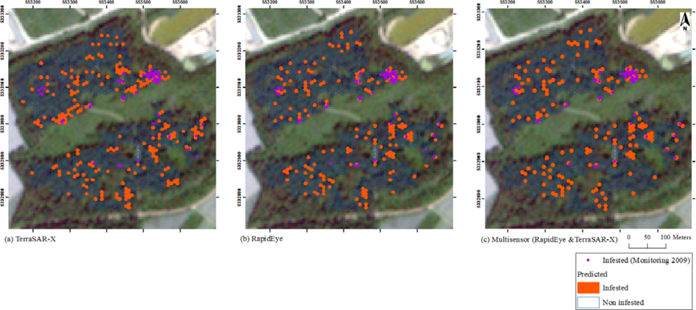
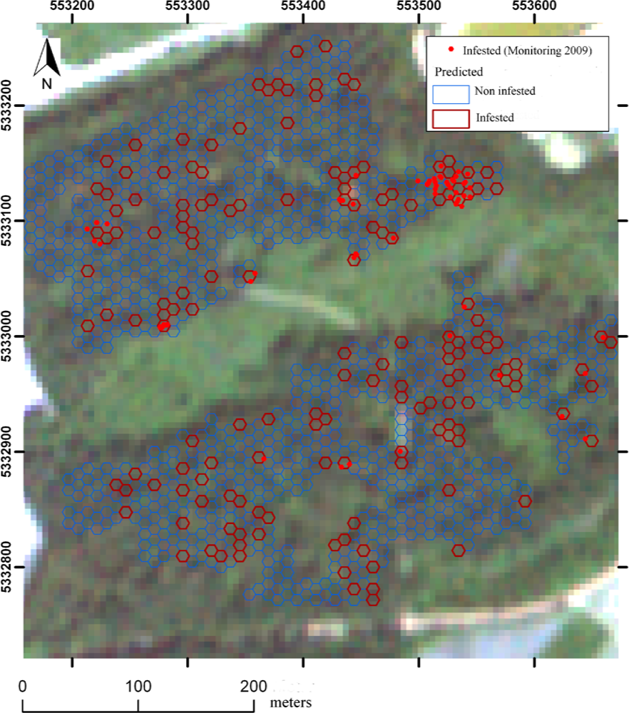
The interpretation of the results was based on two assumptions: (a) the background dataset contained only healthy trees and (b) probabilities of presence greater than 0.5 predicted by a model were classified as bark beetle green attack. However, it should be noted that the model predictions, especially those of ME, are not probabilities of attack in the strict sense of the word. It is more appropriate to interpret them as a relative index where high values represent higher probability of green attack. The reason is that the prevalence of the presence or absence of the green attack at the background locations is unknown [44].
The explanatory variables that were identified as being important by each method were also tested in the other approaches to identify the combination of explanatory variables that resulted in the highest classification accuracy for the three approaches.
The best model was selected consulting Cohen’s Kappa Coefficient (kappa) and the area under the curve (AUC) after leave-one-out cross-validation (to avoid overfitting). Interpretation of the kappa values were based on the categories proposed by Landis and Koch [56] where the classification accuracy of kappa ≤ 0.20 is poor, 0.21 < kappa ≤ 0.40 fair, 0.41< kappa ≤ 0.60 moderate, 0.61 < kappa ≤ 0.80 good, and 0.81 < kappa ≤ 1 very good. The AUC is an assessment of model performance or predictive power [57]. Models with random outcome tend to have AUC values of 0.5, while perfect models have AUC values closer to 1.0. Phillips and Dudik [58] suggested that models with AUC values above 0.75 can be considered useful for predictions.
Finally, a prediction map of bark beetle green attack at the study site was generated. For this purpose, a test area was tessellated into hexagons with the same size of the reference data (78.5 m2, circular plots with a radius of 5 m). The explanatory variables were extracted for each hexagon located within forested area. These values were used as input for the fitted models resulting in a prediction of green attack probability for each polygon. The predictions were displayed in map form and visually compared with the maps of the terrestrial monitoring from 2009 and orthophotos from 2007.

3. Results

In general, plots affected by bark beetle green attack tended to have higher reflectance and radar backscatter than background areas. In addition, the variability of most of the explanatory variables was greater for attacked areas than for the background areas, as can be seen by the larger interquartile distances of plots with green attack. However, the spectral information, as expressed by single explanatory variables, overlapped strongly (Figure 2).
The variable selection implemented in ME was more suitable than the variable selection used for RF and GLM. The RF and GLM models improved when the variables selected by ME were used as explanatory variables instead of the variables selected by RF or GLM. In the final models, ME and RF shared the same explanatory variables, while for the GLM three of these variables were not statistically significant from zero and were therefore not included in the final model (Figure 2).
ME always resulted in models with the highest accuracy compared to GLM and RF. The best model based on the RapidEye image resulted in a kappa of 0.51. The best model based on the TerraSAR-X data resulted in a kappa of 0.23. The highest classification accuracy with a kappa of 0.74 was obtained by combining the spectral information of the two sensors (Table 3). The accuracy of the ME and GLM models were similar whether or not cross-validation was applied. In contrast, the accuracy of RF substantially deteriorated after cross-validation. Estimates of relative contributions of the explanatory variables to the three models calculated with ME are given in Table 4.
An example of the prediction maps obtained with the ME model is displayed in Figure 3 (see also Figure A1). Basically, all areas that contained trees with bark beetle green attack were correctly predicted (no omission errors). However, many commission errors were visible. The visual interpretation of the maps indicated that the most common factors for commission errors were mixed coniferous/deciduous areas and areas close to inner- and outer forest borders.

4. Discussion

The study evaluated the capabilities of RapidEye and TerraSAR-X imagery for the early detection of bark beetle green attack using three different statistical methods.
RapidEye data resulted in moderate classification accuracy when used alone. The reflectance patterns observed were consistent with studies that analyzed the effect of water stress of leaves or needles on the spectral signature [5961]. Higher reflectance values in the visible spectrum are an indicator of vegetation stress [8]. The reduction of chlorophyll b and carotenoids contents in the needles of stressed trees reduces the absorption in the blue band [6265], whereas changes in the concentration of chlorophyll a influences the absorption in the red-edge band more [65,66]. The absorption in the red band is influenced by changes in the chlorophyll a and b concentration [62]. The absorption in the infrared band decreases when persistent stress begins to cause changes in the leaf structure at the cellular level (foliage desiccation) [59].
As opposed to Schweigler [13] who identified bark beetle green attack in the visible spectrum and not in the NIR range, we also used the NIR bands to distinguish between plots affected by green attack attacked and healthy areas (background). This indicates that Schweigler [13] identified trees in an initial stress phase, while areas with trees in the early process of desiccation were identified in the current study.
The NDVI observed within plots affected by green attack and background areas were typical for vegetation with average to good vigor [67]. Plots affected by green attack tended to have higher NDVI than background areas, since the differences of the reflectance between attacked and background areas in the NIR band were considerably greater than the differences in the red band. Similar results were reported by Richardson and Berlyn [59] who compared the reflectance of fresh spruce branches with the reflectance of the same branches three days after cutting. The NDVI values are likely to decrease again once the green attack turns into red attack [68] as consequence of needle loss and decreased tree vitality [69].
The GNDVI and red-edge NDVI were important explanatory variables to discriminate between attacked and background areas when RapidEye data was used alone. These two vegetation indices are known to be well correlated with chlorophyll and carotenoid concentrations [65]. The vegetation indices based on the combination of the red and red-edge bands have been shown to be useful for the estimation of chlorophyll a and b concentrations at leaf and canopy levels because they minimize the effects of the soil reflectance [8] and are less influenced by leaf biomass than the NDVI [7,65].
The use of TerraSAR-X data alone resulted in fair classification accuracy. Because trees attacked by bark beetles become progressively more water stressed due to xylem disruption [68], a possible reduction in the radar backscatter of attacked areas resulting from a decreased dielectric constant of infested trees was expected. This assumption was based on the observations of McDonald et al.[70], who monitored ten trees over several weeks and analyzed the relationship between tree water availability, dielectric constant and radar backscatter. In contrast, current results displayed higher backscatter values in areas with bark beetle attack. However, the interaction mechanism between radar microwaves and trees is not only influenced by the dielectric constant, but also by the crown structure, needle mass and needle orientation, especially in short wavelengths as the X-band [71]. Therefore, the water-stress signal may have been masked by other effects.
The higher standard deviation of the radar backscatter and the large interquartile distance in attacked areas for most of the explanatory variables were likely attributable to higher variances in spectral signatures from trees having different levels of beetle infestation. As shown by Hickey et al.[72], trees with different symptoms of infestation and different health levels have different biochemical compositions, leading to higher degrees of variance in the spectral signature.
Marx [14] analyzed multi-temporal RapidEye data for the detection of stands with bark beetle attack in green and red stages. Similar to this study, he used eight explanatory variables for the classification, including the green and red bands as well as vegetation indices based on the red-edge band, obtaining a cross validated kappa of 0.78 (including green and red attack). Despite the higher spatial resolution, the classification accuracy of green attack in this study was comparable when RapidEye and TerraSAR-X data were combined.
While Hildebrandt ([73]; p. 628) reported that small-scale forest diseases cannot be identified in SAR images, current results showed that SAR data can complement optical data to improve the classification accuracy. Ranson et al.[74] also used SAR and optical satellite data for disturbance recognition in boreal forests. They observed that, although optical imagery was the single best data type for this purpose, the classification accuracy of moderate and severe insect damages was improved by combining optical and SAR images which was corroborated by results from the current study.
Although Wulder et al.[75] found the use of remotely sensed data for detection of bark beetle green attack at endemic level not viable in Canada, results from the current study are promising for the region in which the study was conducted. However, as indicated by other researchers (e.g., [13,68,76]), the spectral reflectance of the bark beetle green attack is too generic to identify this specific stressor. This means that a differential diagnosis of bark beetle green attack by using remote sensing data is limited since other stressors that cause water stress may result in similar spectral signatures. This may partly explain the commission errors in the prediction map. Another reason for incorrect predictions of attack was the high variability of the spectral information in forest borders and areas with mixed tree species. Additionally, the importance of the blue band as an explanatory variable for the identification of attacked areas may contribute to the false classification in areas with mixed coniferous forest because this band has also been shown to be important in distinguishing between coniferous tree species [65].
The sample size of attacked trees was a critical aspect for the supervised classification since it depends heavily on the number and quality of the ground-truth data [77]. The accuracy of GLM and RF are negatively influenced by small sample sizes (e.g., [23,78,79]). The advantage of ME is that it can be fitted with a low number of presence-only observations and that it is able to model possibly non-linearly relationships. Another advantage of ME compared to RF, which was also reported by Guisan et al.[78], was that the accuracy was not affected applying cross-validation. This indicated that RF was more prone to overfitting than ME. It should be noted that ME is conceptually equivalent to a GLM [80]. The reason for the better performance of ME compared to the GLM can be attributed to the transformation and selection of the explanatory variables in the applied software.

5. Conclusions

The following conclusions can be drawn from this case study: (i) detection of bark beetle green attack with fair to good accuracy (kappa of 0.23–0.74) is possible using adequate remote sensing data and modeling approaches, (ii) when used alone, RapidEye data resulted in a higher accuracy (kappa of 0.51) than TerraSAR-X (kappa of 0.23), (iii) the combination of RapidEye and TerraSAR-X resulted in a considerably higher accuracy (kappa of 0.74) than using only one of the sensors, (iv) given the sparse occurrence of trees with bark beetle green attack and the resulting small sample size of presence-only data, the maximum entropy (ME) approach was found to be better suited for classification than random forests (RF) and generalized linear models (GLM).
Remote sensing-based maps indicating the presence of bark beetle green attack could support the current monitoring practice used by the forest service by focusing the terrestrial search of infested trees to areas predicted as attacked. This may reduce costs and improve the efficiency of the monitoring program. Future studies should investigate whether the findings from the current study can be validated on larger areas and in other biomes. Furthermore, to improve the results, future studies should explore the suitability of multi-temporal images and SAR data of other polarizations.

Acknowledgments

We would like to thank two anonymous reviewers for their helpful suggestions. Furthermore, we would like to thank Albrecht Moser, Karl Langlouis and Christof Schoch, Biberach forestry office, for providing access to the study site and for support with the terrestrial monitoring. We appreciated the help of Holger Veit, Department of Forest Protection at the Forest Research Institute of Baden-Württemberg, during field work. We also appreciated the co-operation with Barbara Koch, Department of Remote Sensing and Landscape Information Systems at the University of Freiburg, in the “FoX” and “RaMBOI” projects. TerraSAR-X and RapidEye data were provided by the German Aerospace Centre (DLR) within the “Forest monitoring with TerraSAR-X (FoX)” and the RESA “Rapid Monitoring of Bark beetle and Oak procession moth Infestations (RaMBOI)” projects. This study was partially financed by the European Space Agency (ESRIN/AO/1-5781/08/I-EC).

References and Notes

  1. Lindner, M.; Maroschek, M.; Netherer, S.; Kremer, A.; Barbati, A.; Garcia, J.; Seidl, R.; Delzon, S.; Corona, P.; Kolström, M.; et al. Climate change impacts, adaptive capacity, and vulnerability of European forest ecosystems. Forest Ecol. Manag 2010, 259, 698–709. [Google Scholar]
  2. Meining, S.; Wilpert, K.V.; Schröter, H.; Schäffer, J.; Morgenstern, Y.; Zirlewagen, D. Waldzustandsbericht 2009 der Forstlichen Versuchsund Forschungsanstalt Baden-Württemberg (FVA); ForstBW: Freiburg, Germany, 2010; pp. 1–72. [Google Scholar]
  3. Wulder, M.; White, J.; Coops, N.; Han, T.; Alvarez, M.; Butson, C.; Yuan, X. A Procedure for Mapping and Monitoring Mountain Pine Beetle Red Attack Forest Damage Using Landsat Imagery; Pacific Forestry Centre, Canadian Forest Service, Natural Resources Canada: Victoria, BC, Canada, 2006; pp. 1–40. [Google Scholar]
  4. Deshayes, M.; Guyon, D.; Jeanjean, H.; Stach, N.; Jolly, A.; Hagolle, O. The contribution of remote sensing to the assessment of drought effects in forest ecosystems. Ann. Forest Sci 2006, 63, 579–595. [Google Scholar]
  5. Dong, J.; Zhuang, D.; Huang, Y.; Fu, J. Advances in multi-sensor data fusion: Algorithms and Applications. Sensors 2009, 9, 7771–7784. [Google Scholar]
  6. Xia, J.; Du, P.; Cao, W. Classification of high resolution optical and SAR fusion image using fuzzy knowledge and object-oriented paradigm. Int. Arch. Photogramm. Remote Sens. Spat. Inf. Sci. 2010, XXXVIII-4/C7, 1–5. [Google Scholar]
  7. Eitel, J.; Vierling, L.; Litvak, M.; Long, D.; Schulthess, U.; Ager, A.; Krofcheck, D.; Stoscheck, L. Broadband, red-edge information from satellites improves early stress detection in a New Mexico conifer woodland. Remote Sens. Environ 2011, 115, 3640–3646. [Google Scholar]
  8. Zarco-Tejada, P.; Sepulcre-Cantó, G. Remote Sensing of Vegetation Biophysical Parameters for Detecting Stress Condition and Land Cover Changes. In Estudios de la Zona no Saturada del Suelo Vol. VIII; Juan Vicente Giráldez Cervera y Francisco José Jiménez Hornero: Córdoba, Spain, 2007; pp. 37–44. [Google Scholar]
  9. Roberts, A.; Dragicevic, S.; Northrup, J.; Wolf, S.; Li, Y.; Coburn, C. Mountain Pine Beetle Detection and Monitoring: Remote Sensing Evaluations; FII Operational Report with Reference to Recipient Agreement R2003-0205; Department of Geography, Simon Fraser University: Vancouver, BC, Canada, 2003; pp. 1–45. Available online: http://www.for.gov.bc.ca/hfd/library/fia/html/FIA2003MR271.htm (accessed on 11 November 2012).
  10. Murtha, P.; Wiart, R. PC-based digital analysis of mountain pine beetle current-attacked and non-attacked lodgepole pine. Can. J. Remote Sens 1989, 15, 70–76. [Google Scholar]
  11. Heath, J. Detection of Mountain Pine Beetle Green Attacked Lodgepole Pine Using Compact Airborne Spectrographic Imagery (CASI) Data. 2001; pp. 1–72. Available online: https://circle.ubc.ca/handle/2429/11545 (accessed on 11 November 2012). [Google Scholar]
  12. Roberts, A.; Northrup, J.; Reich, R. Mountain Pine Beetle Detection and Monitoring: Replication Trials for Early Detection. Proceedings of Third International Workshop on the Analysis of Multi-temporal Remote Sensing Images, Biloxi, MS, USA, 16–18 May 2005; pp. 20–24.
  13. Schweigler, P. Früherkennung von Buchdruckerbefall. 2007; pp. 1–73. [Google Scholar]
  14. Marx, A. Erkennung von borkenkäferbefall in fichtenreinbeständen mit multi-temporalen rapideye- satellitenbildern und datamining-techniken. Photogramm. Fernerk. Geoinf 2010, 4, 243–252. [Google Scholar]
  15. Tanase, M.; Santoro, M.; Wegmuller, U.; de la Riva, J.; Perez-Cabello, F. Properties of X-, C- and L-band repeat-pass interferometric SAR coherence in Mediterranean pine forests affected by fires. Remote Sens. Environ 2010, 114, 2182–2194. [Google Scholar]
  16. Tanase, M.; de la Riva, J.; Santoro, M.; Pérez, F.; Kasischke, E. Sensitivity of SAR data to post-fire forest regrowth in Mediterranean and boreal forests. Remote Sens. Environ 2011, 115, 2075–2085. [Google Scholar]
  17. Solberg, S.; Astrup, R.; Lyytikainen-Saarenmaa, P.; Kantola, T.; Holopainen, M.; Kaartinen, H. Testing TerraSAR-X for Forest Disturbance Mapping. Proceedings of 4th TerraSAR-X Science Team Meeting, Oberpfaffenhofen, Germany, 14–16 February 2011; pp. 1–7.
  18. Ackermann, J.; Klaus, M. Erfassung großflächiger Insektenfraßschäden an Kiefer durch Radardaten. AFZ-Der Wald 2011, 6, 20–22. [Google Scholar]
  19. Reid, R. Moisture changes in lodgepole pine before and after attack by the mountain pine beetle. Forestry Chron 1961, 37, 368–375. [Google Scholar]
  20. Wermelinger, B. Ecology and management of the spruce bark beetle Ips typographus—A review of recent research. Forest Ecol. Manag 2004, 202, 67–82. [Google Scholar]
  21. de Jong, J.; de Groot, H.; Klaassen, W.; Kuiper, P. Radar Backscatter Change from an Ash in Relation to Its Hydrological Properties. Proceedings of the IEEE International Geoscience and Remote Sensing Symposium IGARSS 2000, Honolulu, HI, USA, 24–28 July 2000; 7, pp. 2927–2929.
  22. Albertz, J.; Wiggenhage, M. Guide for Photogrammetry and Remote Sensing; Herbert Wichmann Verlag: Berlin und Offenbach, Germany, 2009; p. 334. [Google Scholar]
  23. Hernandez, PA.; Graham, C.; Master, L.; Albert, D. The effect of sample size and species characteristics on performance of different species distribution modeling methods. Ecography 2006, 29, 773–785. [Google Scholar]
  24. Coggins, S.; Coops, N.; Wulder, M. Improvement of low level bark beetle damage estimates with adaptive cluster sampling. Silva Fenn 2010, 44, 289–301. [Google Scholar]
  25. Valavanis, V.; Pierce, G.; Zuur, A.; Palialexis, A.; Saveliev, A.; Katara, I.; Wang, J. Modelling of essential fish habitat based on remote sensing, spatial analysis and GIS. Hydrobiologia 2008, 612, 5–20. [Google Scholar]
  26. Elith, J.; Phillips, S.; Hastie, T.; Dudk, M.; Chee, Y.; Yates, C. A statistical explanation of MaxEnt for ecologists. Divers. Distrib 2011, 17, 43–57. [Google Scholar]
  27. Forst, BW. Forest inventory in the forest district of Biberach (internal digital database). 2003. [Google Scholar]
  28. RapidEye AG. RapidEye Standard Image Product Specifications; RapidEye AG: Brandenburg an der Havel, Germany, 2011; pp. 1–54. [Google Scholar]
  29. Düring, R.; Koudogbo, F.; Weber, M. TerraSAR-X and TanDEM-X: Revolution in Spaceborne Radar. Int .Arch. Photogramm. Remote Sens. Spat. Inf. Sci 2008, 37, 227–234. [Google Scholar]
  30. DLR. TerraSAR-X, Ground Segment, Basic Products Specification Document; Deutsches Zentrum für Luft und Raumfahrt: Oberpfaffenhofen, Germany, 2006; pp. 1–45. [Google Scholar]
  31. Nowak, J.; Tokarczyk, P. Analysis of the Geometric Quality of the LPIS-Based RapidEye Level 3A; JRC Scientific and Technical Reports; JRC European Commission: Ispra, Italy, 2010; pp. 1–47. [Google Scholar]
  32. Jackson, R.; Huete, R. Interpreting vegetation indices. Preventive Veterinary Medicine 1991, 11, 185–200. [Google Scholar]
  33. Infoterra. Radiometric Calibration of TerraSAR-X Data; Infoterra GmbH: Friedrichshafen, Germany, 2008; pp. 1–16. [Google Scholar]
  34. Schleyer, A. Das Laserscan-DGM von Baden-Wuerttemberg. Photogramm. Week 2001, 1, 217–225. [Google Scholar]
  35. Weinacker, H.; Koch, B.; Weinacker, R. TREESVIS: A Software System for Simultaneous ED-Real-Time Visualisation of DTM, DSM, Laser Raw Data, Multispectral Data, Simple Tree and Building Models. Proceedings of the ISPRS Working Group VIII (2), Freiburg, Germany, 3–6 October 2004; pp. 90–95.
  36. Wegmüller, U. Automated Terrain Corrected SAR Geocoding. Proceedings of the IEEE International Geoscience and Remote Sensing Symposium IGARSS’99, Hamburg, Germany, 28 June–2 July 1999; pp. 1712–1714.
  37. Werner, C.; Wegmüller, U.; Strozzi, T.; Wiesmann, A. Gamma SAR and Interferometry Software. Proceedings of ERS-ENVISAT Symposium, Gothenburg, Sweden, 16–20 October 2000; pp. 1–9.
  38. Rouse, J.; Hass, R.; Schell, J.; Harlan, C. Monitoring the Vernal Advancement of Retrogradation (Greenwave Effect) of Natural Vegetation. NASA Final Report E75-10354, NASA-CR-144661, RSC-1978-4. 1974, pp. 1–390. Available online: http://ntrs.nasa.gov/search.jsp?R=19750020419 (accessed on 11 November 2012).
  39. Buschmann, C.; Nagel, E. In vivo spectroscopy and internal optics of leaves as basis for remote sensing of vegetation. Int. J. Remote Sens 1993, 14, 711–722. [Google Scholar]
  40. Gitelson, A.; Merzlyak, M. Remote estimation of chlorophyll content in higher plant leaves. Int. J. Remote Sens 1996, 18, 2691–2697. [Google Scholar]
  41. Barnes, E.; Richard, S.; Colaizzi, P.; Haberland, J.; Kostrzewski, M.; Waller, P.; Choi, C. Coincindent Detection of Crop Water Stress, Nitrogen Status and Canopy Density Using Ground-Based Multispectral Data. Proceedings of the Fifth International Conference on Precision Agriculture, Bloomington, IN, USA, 16–19 July 2000; pp. 1–15.
  42. Gitelson, A.; Viña, A.; Ciganda, V.; Rundquist, D.; Arkebauer, T. Remote estimation of canopy chlorophyll content in crops. Geophys. Res. Lett 2005, 32, L08403. [Google Scholar] [CrossRef]
  43. Phillips, S.; Anderson, R.; Schapire, R. Maximum entropy modeling of species geographic distributions. Ecol. Model 2006, 190, 231–259. [Google Scholar]
  44. Venables, W.; Ripley, B. Generalized Linear Models. In Modern Applied Statistics with S. Statistics and Computing, 4th ed.; Springer: New York, NY, USA, 2002; pp. 183–208. [Google Scholar]
  45. McCullagh, P.; Nelder, J. Generalized Linear Models, 2nd ed.; Chapman and Hall: London, UK, 1989; pp. 1–506. [Google Scholar]
  46. R Development Core Team. R A Language and Environment for Statistical Computing. 2010. Available online: http://www.r-project.org/ (accessed on 15 September 2012).
  47. Pinheiro, J.; Bates, D. Mixed-Effects Models in S and S-PLUS; Springer: New York, NY, USA, 2000; pp. 1–523. [Google Scholar]
  48. Braunisch, V.; Patthey, P.; Arlettaz, R. Spatially explicit modeling of conflict zones between wildlife and snow sports: Prioritizing areas for winter refuges. Ecol. Appl 2011, 21, 955–967. [Google Scholar]
  49. Faraway, J. Practical Regression and Anova Using R. 2002. Available online: http://cran.r-project.org/doc/contrib/Faraway-PRA.pdf (accessed on 15 September 2012).
  50. Phillips, S. A Brief Tutorial on Maxent; 2005; Available online: www.cs.princeton.edu/~schapire/-maxent/tutorial/tutorial.doc (accessed on 15 September 2012).
  51. Breiman, L. Random forests. Mach. Learn 2001, 45, 5–32. [Google Scholar]
  52. Morgan, J.; Sonquist, J. Problem in the analysis of survey data, and a proposal. J. Am. Statist. Assoc 1963, 58, 415–434. [Google Scholar]
  53. Breidenbach, J.; Nothdurft, A.; Kändler, G. Comparison of nearest neighbour approaches for small area estimation of tree species-specific forest inventory attributes in central Europe using airborne laser scanner data. Eur. J. Forest Res 2010, 129, 833–846. [Google Scholar]
  54. Crookston, N.; Finley, A. yaImpute: An R Package for k-NN Imputation. J. Statist. Softw 2008, 23, 1–16. [Google Scholar]
  55. Strobl, C.; Boulesteix, A.; Kneib, T.; Augustin, T.; Zeileis, A. Conditional variable importance for random forests. BMC Bioinf 2008. [Google Scholar] [CrossRef]
  56. Landis, J.; Koch, G. The measurement of observer agreement for categorical data. Biometrics 1977, 33, 159–174. [Google Scholar]
  57. Boyce, M.; Vernier, P.; Nielsen, S.; Schmiegelow, F. Evaluating resource selection functions. Ecol. Model 2002, 157, 281–300. [Google Scholar]
  58. Phillips, S.; Dudik, M. Modeling of species distributions with Maxent: New extensions and a comprehensive evaluation. Ecography 2008, 31, 161–175. [Google Scholar]
  59. Richardson, A.; Berlyn, G. Changes in foliar spectral reflectance and chlorophyll fluorescence of four temperate species following branch cutting. Tree Physiol 2002, 22, 499–506. [Google Scholar]
  60. Carter, G. Responses of leaf spectral reflectance to plant stress. Am. J. Bot 1993, 80, 239–243. [Google Scholar]
  61. Carter, G. Primary and secondary effects of water content on the spectral reflectance of leaves. Am. J. Bot 1991, 78, 916–924. [Google Scholar]
  62. Lichtenthaler, H.; Rinderle, U. The role of chlorophyll fluorescence in the detection of stress conditions in plants. CRC Critical Rev. Anal. Chem 1988, 19, 29–85. [Google Scholar]
  63. Zwiggelaar, R. A review of spectral properties of plants and their potential use for crop/weed discrimination on row-crops. Crop Protect 1998, 17, 189–206. [Google Scholar]
  64. Stockburger, K.; Mitchell, A. Photosynthetic Pigments: A Bibliography; BC-X-383; Information Report; Canadian Forest Service, Pacific Forestry Centre: Victoria, BC, Canada, 1999; pp. 1–30. [Google Scholar]
  65. Mohammed, G.; Noland, T.; Irving, D.; Sampson, P.; Zarco-Tejada, P.; Miller, J. Natural and Stress-Induced Effects on Leaf Spectral Reflectance in Ontario Species; Ontario Forest Research Institute: Marie, ON, Canada, 2000; pp. 1–34. [Google Scholar]
  66. Schelling, K.; Schulthess, U. Abschaetzung des Chlorophyllgehaltes von Pflanzenbestaenden mit RapidEye Satellitenbilddaten. Proceedings of Precision Agriculture Reloaded; Informationsgestuetzte Landwirtschaft. 30 GIL-Jahrestagung, Stuttgart, Germany, 24–25 February 2010; pp. 167–170.
  67. Bonneau, L.; Shields, K.; Civco, D. Using satellite images to classify and analyze the health of hemlock forests infested by the hemlock woolly adelgid. Biol. Invasion 1999, 1, 255–267. [Google Scholar]
  68. Niemann, K.; Visintini, F. Assessment of Potential for Remote Sensing Detection of Bark Beetle-Infested Areas during Green Attack: A Literature Review; Natural Resources Canada, Canadian Forest Service: Victoria, BC, Canada, 2005; pp. 1–14. Available online: http://cfs.nrcan.gc.ca/pubwarehouse/pdfs/25269.pdf (accessed on 15 September 2012).
  69. Barsch, H.; Steinhardt, U.; Soellner, R. The development of forest damage—Control and prognosis on the basis of remote sensing data. GeoJournal 1994, 32, 39–46. [Google Scholar]
  70. McDonald, K.; Zimmermann, R.; Way, J. An Investigation of the Relationship between Tree Water Potential and Dielectric Constant. Proceedings of the IEEE International Geoscience and Remote Sensing Symposium IGARSS’92, Houston, TX, USA, 26–29 May 1992; pp. 523–525.
  71. Hoekman, D. Radar backscattering of forest stands. Int. J. Remote Sens 1985, 6, 325–343. [Google Scholar]
  72. Hickey, J.; Birnie, R.; Zhao, M. Oleoresin, Chemistry and Spectral Reflectance in Stressed Lodgepole and White Bark Pine, Mammoth Mountain, California. Summary of the Tenth Annual JPL Airborne Earth Science Workshop, Pasadena, CA, USA, 27 February–2 March 2001; pp. 1–10.
  73. Hildebrandt, G. Fernerkundung und Luftbildmessung: Für Forstwirtschaft, Vegetationskartierung und Landschaftsoekologie; Wichmann: Heidelberg, Germany, 1996. [Google Scholar]
  74. Ranson, K.; Kovacs, K.; Sun, G.; Kharuk, V. Disturbance recognition in the boreal forest using radar and Landsat-7. Can. J. Remote Sens 2003, 29, 271–285. [Google Scholar]
  75. Wulder, M.; White, J.; Carroll, A.; Coops, N. Challenges for the operational detection of mountain pine beetle green attack with remote sensing. For. Chron 2009, 85, 32–38. [Google Scholar]
  76. Carter, G.; Knapp, A. Leaf optical properties in higher plants: linking spectral characteristics to stress and chlorophyll concentration. Am. J. Bot 2001, 88, 677–684. [Google Scholar]
  77. Xie, Y.; Sha, Z.; Yu, M. Remote sensing imagery in vegetation mapping: a review. J. Plant Ecol 2008, 1, 9–23. [Google Scholar]
  78. Guisan, A.; Zimmermann, N.; Elith, J.; Graham, C.; Phillips, S.; Peterson, A. What matters for predicting the occurrences of trees: techniques, data, or species characteristics? Ecol. Monogr 2007, 77, 615–630. [Google Scholar]
  79. Meynard, C.; Quinn, J. Predicting species distributions: a critical comparison of the most common statistical models using artificial species. J. Biogeogr 2007, 34, 1455–1469. [Google Scholar]
  80. Renner, I.; Warton, D. Equivalence of MAXENT and poisson point process models for species distribution modeling in ecology. Biometrics 2013, 69, 274–281. [Google Scholar]

Appendix

Figure A1. ME predication maps for bark beetle green attack (RapidEye image in background).
Remotesensing 05 01912fa1
Figure 1. (a) Location of the study site Biberach with the surrounding countries and German federal states (BW = Baden-Württemberg, BY = Bavaria, HE = Hesse, RP = Rhineland-Palatinate) (UTM coordinates zone 32N in the margins). (b) Forest district with the location of the satellite images and reference data. (c) Location of the tree groups with pheromone dispensers (orthophotograph in the background).
Remotesensing 05 01912f1
Figure 2. Boxplots of explanatory variables for the models with the highest classification accuracy. The individual figure captions indicate in which model type the explanatory variable is used (RE = RapidEye, TSX = TerraSAR-X, ME = maximum entropy, RF = random forest, GLM = generalized linear model).
Remotesensing 05 01912f2
Figure 3. Multisensor ME prediction map for bark beetle green attack (RapidEye image in background).
Remotesensing 05 01912f3
Table 1. Characteristics of the satellite images.
RapidEyeTerraSAR-X
Acquisition date25 May 0924 May 09
Extent25 by 25 km (41% coverage)10 by 10 km
Orbital directionDescendingDescending
Incidence angle6.7°37.5°
Illumination azimuth angle175.5°---
Illumination elevation angle62.9°---
Pixel size5 m2 m
Spatial resolution6.5 mSlant range resolution: 1.18 m
Azimuth resolution: 2.05 m
Spectral coverageBlue: 410–510 nmX-band
Green: 520–590 nm---
Red: 630–690 nm---
Red-edge: 690–730 nm---
Near infrared: 760–850 nm---
Radiometric resolution12 bit16 bit
Table 2. Vegetation indices calculated from the RapidEye data.
IndexFormula
NDVI [38] NIR Red NIR + Red
Red-edge Green NDVI [39] ( Red-edge ) Green ( Red-edge ) + Green
Green NDVI (GNDVI) [40] NIR Green NIR + Green
Red-edge index (NDRE) [41] NIR ( Red-edge ) NIR + ( Red-edge )
Chlorophyll Green Model (CGM) [42] NIR Green 1
Chlorophyll Red-edge Model (CRM) [42] NIR ( Red-edge ) 1
Red-edge NDVI ( Red-edge ) Red ( Red-edge ) + Red
Table 3. Confusion matrices and performance of the best models after cross validation (0 = Background (n = 230 plots); 1 = Green attack (n = 15 plots); ME = maximum entropy; RF = random forest; GLM = generalized linear model).
TerraSAR-XRapidEyeMultisensor (TerraSAR-X & RapidEye)

MERFGLM

PredictedObserved
0101010101
02067220522742281022813
124810103112522
PA (%)89.653.395.766.798.773.399.133.399.113.3
UA (%)96.725.097.850.098.378.695.871.494.650.0
OA (%)87.393.997.195.193.9

AUC0.700.800.800.660.56
Kappa0.280.50.740.430.19
Kappa 95% CI0.04–0.50.3–0.760.55–0.930.11–0.74(−0.2) −0.58
*The overall accuracy (OA) was always large due to the extremely imbalanced sample data where more than 90% of the observations were background data.
Table 4. Importance of the explanatory variables in the ME models.
TerraSAR-XRapidEyeMultisensor
Variable (Metric)Contribution (%)
Backscatter (Q3)39.516.9
Backscatter (Q2)22.9
Backscatter (SD)18.814.5
Backscatter (Q1)10.7
Backscatter (max)8.1
Blue band (max and min)31.214.4
GNDVI (max)28
NDVI (max)17.1339.1
Red-edge band (min)11.912
Red-edge NDVI (mean)8.3
NIR band (min)3.33.1

Sum100100100

