Generating Virtual Images from Oblique Frames

 ,
,
Abstract
:1. Introduction
2. Background
2.1. Camera Calibration
2.2. Multi-Head Camera Calibration
3. Methodology
3.1. Camera Calibration with RO Constraints
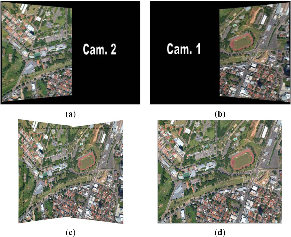
3.2. Image Rectification
3.3. Image Registration
3.4. Images Fusion
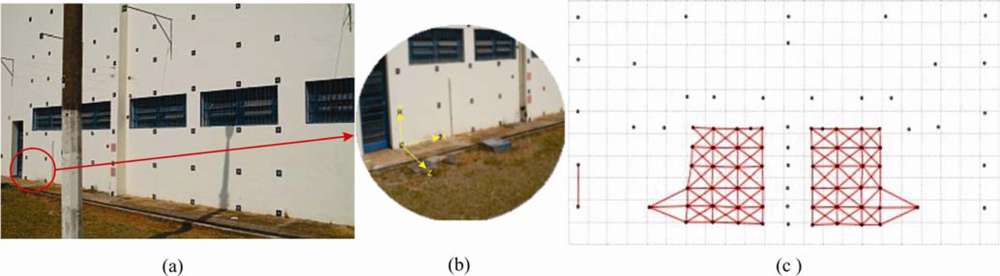
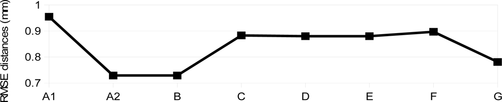
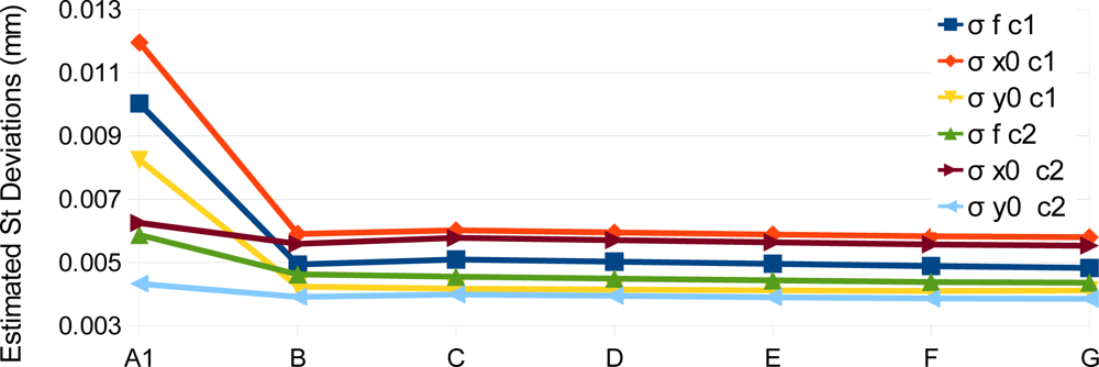
4. Experimental Assessment
5. Conclusions
Acknowledgments
References
- Ruy, R.S.; Tommaselli, A.M.G.; Galo, M.; Hasegawa, J.K.; Reis, T.T. Accuracy Analysis of Modular Aerial Digital System SAAPI in Projects of Large Areas. Proceedings of EuroCow2012—International Calibration and Orientation Workshop, Castelldefels, Spain, 8–10 February 2012.
- Mostafa, M.M.R.; Schwarz, K.-P. A multi-sensor system for airborne image capture and georreferencing. Photogramm. Eng. Remote Sensing 2000, 66, 1417–1423. [Google Scholar]
- Zeitler, D.W.; Doerstel, C.; Jacobsen, D.K. Geometric Calibration of the DMC: Method and Results. Proceedings of the ISPRS Commission I/Pecora 15 Conference, Denver, CO, USA, 10–15 November 2002; pp. 324–333.
- Hunt, E.R.; Hively, W.D.; Fujikawa, S.J.; Linden, D.S.; Daughtry, C.S.T.; McCarty, G.W. Acquisition of NIR-green-blue digital photographs from unmanned aircraft for crop monitoring. Remote Sens 2010, 2, 290–305. [Google Scholar]
- Ritchie, G.L.; Sullivan, D.G.; Perry, C.D.; Hook, J.E.; Bednarz, C.W. Preparation of a low-cost digital camera system for remote sensing. Appl. Eng. Agric 2008, 24, 885–896. [Google Scholar]
- Chao, H.; Jensen, A.M.; Han, Y.; Chen, Y.; McKee, M. AggieAir: Towards Low-Cost Cooperative Multispectral Remote Sensing Using Small Unmanned Aircraft Systems. In Advances in Geoscience and Remote Sensing; Jedlovec, G., Ed.; InTech: Rijeka, Croatia, 2009. [Google Scholar] [CrossRef]
- Schoonmaker, J.; Podobna, Y.; Boucher, C.; Saggese, S.; Runnels, D. Multichannel imaging in remote sensing. Proc. SPIE 2009. [Google Scholar] [CrossRef]
- Hakala, T.; Suomalainen, J.; Peltoniemi, J.I. Acquisition of bidirectional reflectance factor dataset using a micro unmanned aerial vehicle and a consumer camera. Remote Sens 2010, 2, 819–832. [Google Scholar]
- Laliberte, A.S.; Goforth, M.A.; Steele, C.M.; Rango, A. Multispectral remote sensing from unmanned aircraft: Image processing workflows and applications for rangeland environments. Remote Sens 2011, 3, 2529–2551. [Google Scholar]
- D’Oleire-Oltmanns, S.; Marzolff, I.; Peter, K.D.; Ries, J.B. Unmanned Aerial Vehicle (UAV) for monitoring soil erosion in Morocco. Remote Sens 2012, 4, 3390–3416. [Google Scholar]
- Grenzdörffer, G.; Niemeyer, F.; Schmidt, F. Development of Four Vision Camera System for a Micro-UAV. Proceedings of XXII ISPRS Congress, Melbourne, Australia, 25 August–1 September 2012; pp. 369–374.
- Yang, C. A high-resolution airborne four-camera imaging system for agricultural remote sensing. Comput. Electron. Agric 2012, 88, 13–24. [Google Scholar]
- Holtkamp, D.J.; Goshtasby, A.A. Precision registration and mosaicking of multicamera images. IEEE Trans. Geosci. Remote Sens 2009, 47, 3446–3455. [Google Scholar]
- Petrie, G. Systematic oblique aerial photography using multiple digital frame camera. Photogramm. Eng. Remote Sensing 2009, 75, 102–107. [Google Scholar]
- Tommaselli, A.M.G.; Galo, M.; Marcato, J., Jr.; Ruy, R.S.; Lopes, R.F. Registration and Fusion of Multiple Images Acquired with Medium Format Cameras. Proceedings of the Canadian Geomatics Conference 2010 and Symposium of Commission I, Calgary, AB, Canada, 15–18 June 2010.
- Tommaselli, A.M.G.; Moraes, M.V.A.; Marcato Junior, J.; Caldeira, C.R.T.; Lopes, R.F.; Galo, M. Using Relative Orientation Constraints to Produce Virtual Images from Oblique Frames. Proceedings of XXII ISPRS Congress, Melbourne, Australia, 25 August–1 September 2012; pp. 61–66.
- Brown, D. Close-range camera calibration. Photogramm. Eng 1971, 37, 855–866. [Google Scholar]
- Clarke, T.; Fryer, J. The development of camera calibration methods and models. Photogramm. Rec 1998, 16, 51–66. [Google Scholar]
- Habib, A.F.; Morgan, M.F. Automatic calibration of low-cost digital cameras. Opt. Eng 2003, 42, 948–955. [Google Scholar]
- Merchant, D.C. Analytical Photogrammetry: Theory and Practice; Ohio State University: Columbus, OH, USA, 1979. [Google Scholar]
- Choi, K.; Lee, I. A Sequential aerial triangulation algorithm for real-time georeferencing of image sequences acquired by an airborne multi-sensor system. Remote Sens 2013, 5, 57–82. [Google Scholar]
- Nakano, K.; Chikatsu, H. Camera-variant calibration and sensor modeling for practical photogrammetry in archeological sites. Remote Sens 2011, 3, 554–569. [Google Scholar]
- Zhuang, H. A self-calibration approach to extrinsic parameter estimation of stereo cameras. Robot. Auton. Syst 1995, 15, 189–197. [Google Scholar]
- He, G.; Novak, K.; Feng, W. Stereo camera system calibration with relative orientation constraints. Proc. SPIE 1994. [Google Scholar] [CrossRef]
- King, B.A. Methods for the photogrammetric adjustment of bundles of constrained stereopairs. Int. Arch. Photogramm. Remote Sens. Spat. Inf. Sci 1994, 30, 473–480. [Google Scholar]
- King, B.A. Bundle adjustment of constrained stereopairs-mathematical models. Geomat. Res. Austr 1995, 63, 67–92. [Google Scholar]
- El-Sheimy, N. The Development of VISAT—A Mobile Survey System for GIS Applications. 1996. [Google Scholar]
- Tommaselli, A.M.G; Alves, A.O. Calibração de uma Estereocâmara Baseada em vídeo. In Séries em Ciências Geodésicas—30 Anos de Pós-Graduação em Ciências Geodésicas no Brasil; Universidade Federal do Paraná: Curitiba, PR, Brazil, 2001; Volume 1, pp. 199–213. [Google Scholar]
- Tommaselli, A.; Galo, M.; Bazan, W.; Ruy, R.; Junior, J.M. Simultaneous Calibration of Multiple Camera Heads with Fixed Base Constraint. Proceedings of the 6th International Symposium on Mobile Mapping Technology, Presidente Prudente, SP, Brazil, 21–24 July 2009.
- Lerma, J.L.; Navarro, S.; Cabrelles, M.; Seguí, A.E. Camera calibration with baseline distance constraints. Photogramm. Rec 2010, 25, 140–158. [Google Scholar]
- Blázquez, M.; Colomina, I. Fast AT: A simple procedure for quasi direct orientation. ISPRS J. Photogramm 2012, 71, 1–11. [Google Scholar]
- Mikhail, E.M.; Ackermann, F.E. Observations and Least Squares; University Press of America: New York, NY, USA, 1983. [Google Scholar]


| Cameras | Fuji S3 Pro |
|---|---|
| Sensor | CCD − 23.0 × 15.5 mm |
| Number of pixels | 4,256 × 2,848 (12 MP) |
| Pixel size (mm) | 0.0054 |
| Focal length (mm) | 28.4 |
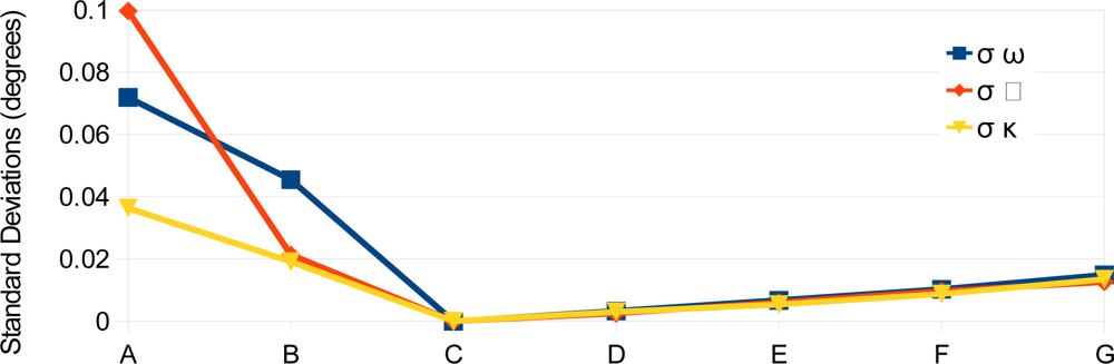
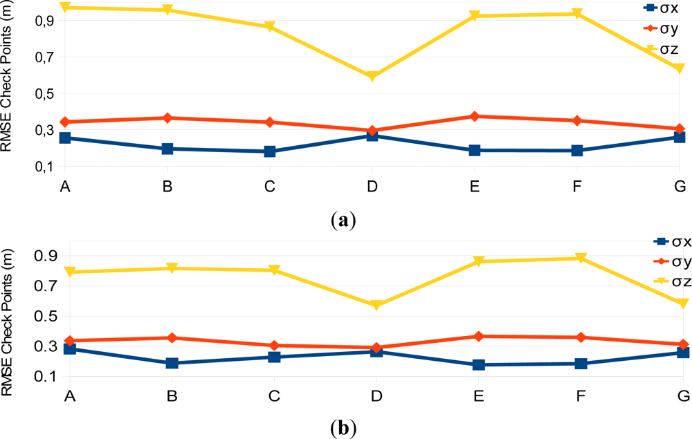
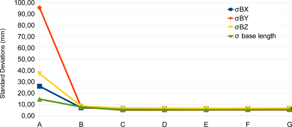
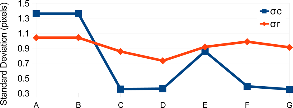
| Experiment | A1 and A2 | B | C | D | E | F | G |
|---|---|---|---|---|---|---|---|
| RO Constraints | Single camera calib. | N | Y | Y | Y | Y | Y |
| Variation of the RO angular elements | - | - | 1″ | 10″ | 15″ | 30″ | 1′ |
| Variation of the base components (mm) | - | - | 1 | 1 | 1 | 1 | 1 |
Share and Cite
Tommaselli, A.M.G.; Galo, M.; De Moraes, M.V.A.; Marcato, J., Jr.; Caldeira, C.R.T.; Lopes, R.F. Generating Virtual Images from Oblique Frames. Remote Sens. 2013, 5, 1875-1893. https://doi.org/10.3390/rs5041875
Tommaselli AMG, Galo M, De Moraes MVA, Marcato J Jr., Caldeira CRT, Lopes RF. Generating Virtual Images from Oblique Frames. Remote Sensing. 2013; 5(4):1875-1893. https://doi.org/10.3390/rs5041875
Chicago/Turabian StyleTommaselli, Antonio M. G., Mauricio Galo, Marcus V. A. De Moraes, José Marcato, Jr., Carlos R. T. Caldeira, and Rodrigo F. Lopes. 2013. "Generating Virtual Images from Oblique Frames" Remote Sensing 5, no. 4: 1875-1893. https://doi.org/10.3390/rs5041875
APA StyleTommaselli, A. M. G., Galo, M., De Moraes, M. V. A., Marcato, J., Jr., Caldeira, C. R. T., & Lopes, R. F. (2013). Generating Virtual Images from Oblique Frames. Remote Sensing, 5(4), 1875-1893. https://doi.org/10.3390/rs5041875