Water Body Distributions Across Scales: A Remote Sensing Based Comparison of Three Arctic Tundra Wetlands


Abstract
:1. Introduction
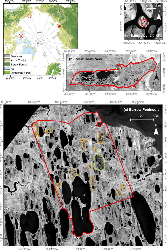
2. Study Areas
3. Material and Methods
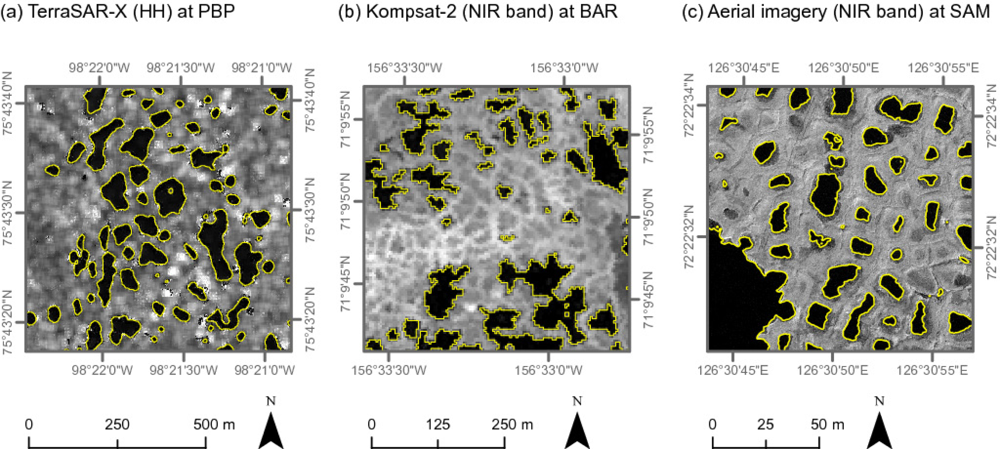
3.1. Processing of Remote Sensing Data
3.1.1. VNIR Aerial Imagery of SAM
3.1.2. TerraSAR-X and SPOT-5 Imagery of PBP
3.1.3. KOMPSAT-2 Imagery of BAR
3.1.4. Landsat-5 Thematic Mapper (TM)
3.1.5. MODIS Water Mask
3.2. Accuracy Assessment of Water Body Classification
3.3. Subpixel Analysis of Landsat Surface Albedo
4. Results
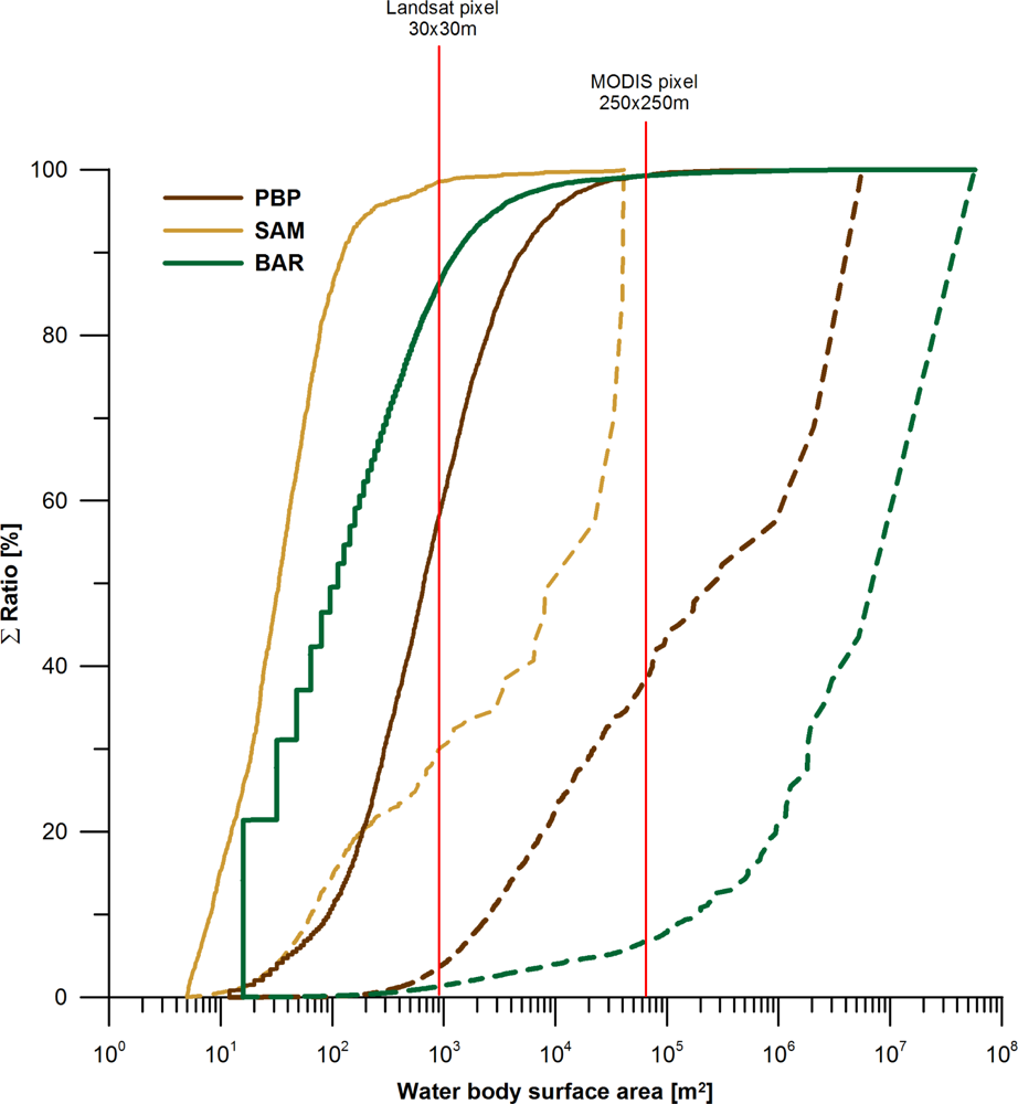
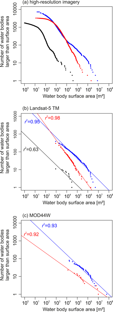
4.1. Abundance and Size Distribution of Water Bodies
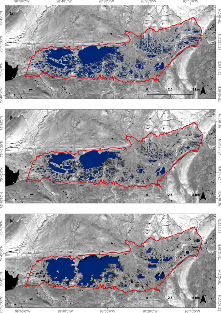
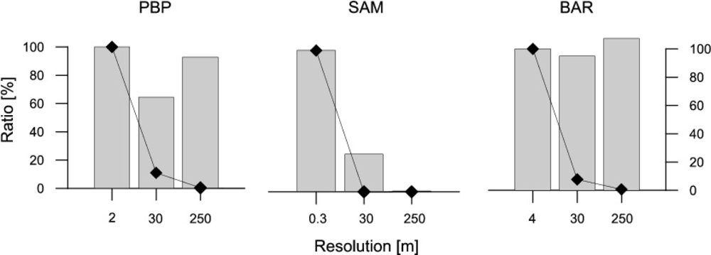
4.2. Effect of Scale on Water Body Mapping
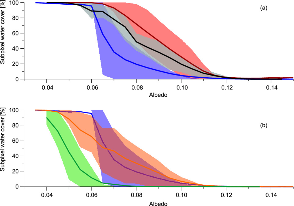
4.3. Subpixel Analysis of Landsat Albedo
5. Discussion
5.1. Size Distribution of Ponds and Lakes Across Scales
5.2. Albedo as an Estimator of Subpixel Water Cover
5.3. Implementation of an Albedo–SWC Function
6. Conclusions
Acknowledgments
References
- Walker, D.; Raynolds, M.; Daniëls, F.; Einarsson, E.; Elvebakk, A.; Gould, W.; Katenin, A.; Kholod, S.; Markon, C.; Melnikov, E.; et al. The circumpolar Arctic vegetation map. J. Veg. Sci. 2005, 16, 267–282. [Google Scholar]
- Tarnocai, C.; Canadell, J.; Schuur, E.; Kuhry, P.; Mazhitova, G.; Zimov, S. Soil organic carbon pools in the northern circumpolar permafrost region. Glob. Biogeochem. Cy. 2009, 23. [Google Scholar] [CrossRef]
- McGuire, A.; Anderson, L.; Christensen, T.; Dallimore, S.; Guo, L.; Hayes, D.; Heimann, M.; Lorenson, T.; Macdonald, R.; Roulet, N. Sensitivity of the carbon cycle in the Arctic to climate change. Ecol. Monogr. 2009, 79, 523–555. [Google Scholar]
- Chapin, F.S., III; McGuire, A.D.; Randerson, J.; Pielke, R.; Baldocchi, D.; Hobbie, S.E.; Roulet, N.; Eugster, W.; Kasischke, E.; Rastetter, E.B. Arctic and boreal ecosystems of western North America as components of the climate system. Glob. Chang. Biol. 2000, 6, 211–223. [Google Scholar]
- Avis, C.A.; Weaver, A.J.; Meissner, K.J. Reduction in areal extent of high-latitude wetlands in response to permafrost thaw. Nat. Geosci. Lett. 2011, 4, 444–448. [Google Scholar]
- Jorgenson, M.; Racine, C.; Walters, J.; Osterkamp, T. Permafrost degradation and ecological changes associated with a warmingclimate in central Alaska. Clim. Chang. 2001, 48, 551–579. [Google Scholar]
- Walter, K.; Zimov, S.; Chanton, J.; Verbyla, D.; Chapin, F. Methane bubbling from Siberian thaw lakes as a positive feedback to climate warming. Nature 2006, 443, 71–75. [Google Scholar]
- Yoshikawa, K.; Hinzman, L.D. Shrinking thermokarst ponds and groundwater dynamics in discontinuous permafrost near Council, Alaska. Permafr. Periglac. Process. 2003, 14, 151–160. [Google Scholar]
- Smith, L.; Sheng, Y.; MacDonald, G.; Hinzman, L. Disappearing Arctic lakes. Science 2005, 308, 1429. [Google Scholar]
- Smol, J.P.; Douglas, M.S.V. Crossing the final ecological threshold in high Arctic ponds. Proc. Natl. Acad. Sci. USA 2007, 104, 12395–12397. [Google Scholar]
- Emmerton, C.; Lesack, L.; Marsh, P. Lake abundance, potential water storage, and habitat distribution in the Mackenzie River Delta, western Canadian Arctic. Water Resour. Res. 2007, 43, W05419. [Google Scholar] [CrossRef]
- Grosse, G.; Romanovsky, V.; Walter, K.; Morgenstern, A.; Lantuit, H.; Zimov, S. Distribution of Thermokarst Lakes and Ponds at Three Yedoma Sites in Siberia. Proceedings of the Ninth International Conference on Permafrost, Fairbanks, AK, USA, 29 June–3 July 2008; pp. 551–556.
- Muster, S.; Langer, M.; Heim, B.; Westermann, S.; Boike, J. Subpixel heterogeneity of ice-wedge polygonal tundra: A multi-scale analysis of land cover and evapotranspiration in the Lena River Delta, Siberia. Tellus B 2012, 64, 17301. [Google Scholar] [CrossRef]
- Laurion, I.; Vincent, W.; MacIntyre, S.; Retamal, L.; Dupont, C.; Francus, P.; Pienitz, R. Variability in greenhouse gas emissions from permafrost thaw ponds. Limnol. Oceanogr. 2010, 55, 115–133. [Google Scholar]
- Abnizova, A.; Siemens, J.; Langer, M.; Boike, J. Small ponds with major impact: The relevance of ponds and lakes in permafrost landscapes to carbon dioxide emissions. Glob. Biogeochem. Cy. 2012, 26, 1–9. [Google Scholar]
- Lehner, B.; Döll, P. Development and validation of a global database of lakes, reservoirs and wetlands. J. Hydrol. 2004, 296, 1–22. [Google Scholar]
- Frey, K.; Smith, L. How well do we know Northern land cover? Comparison of four global vegetation and wetland products with a new ground-truth database for West Siberia. Glob. Biogeochem. Cy. 2007, 21, 1–25. [Google Scholar]
- Ozesmi, S.; Bauer, M. Satellite remote sensing of wetlands. Wetl. Ecol. Manag. 2002, 10, 381–402. [Google Scholar]
- Brown, L.; Young, K. Assessment of three mapping techniques to delineate lakes and ponds in a Canadian High Arctic wetland complex. Arctic 2009, 59, 283–293. [Google Scholar]
- Pflugmacher, D.; Krankina, O.; Cohen, W.; Friedl, M.; Sulla-Menashe, D.; Kennedy, R.; Nelson, P.; Loboda, T.; Kuemmerle, T.; Dyukarev, E.; et al. Comparison and assessment of coarse resolution land cover maps for Northern Eurasia. Remote Sens. Environ. 2011, 115, 3539–3553. [Google Scholar]
- Weiss, D.; Crabtree, R. Percent surface water estimation from MODIS BRDF 16-day image composites. Remote Sens. Environ. 2011, 115, 2035–2046. [Google Scholar]
- Watts, J.; Kimball, J.; Jones, L.; Schroeder, R.; McDonald, K. Satellite Microwave remote sensing of contrasting surface water inundation changes within the Arctic–Boreal Region. Remote Sens. Environ. 2012, 127, 223–236. [Google Scholar]
- Hope, A. Estimating lake area in an Arctic landscape using linear mixture modelling with AVHRR data. Int. J. Remote Sens. 1999, 20, 829–835. [Google Scholar]
- Olthof, I.; Fraser, R. Mapping northern land cover fractions using Landsat ETM+. Remote Sens. Environ. 2007, 107, 496–509. [Google Scholar]
- Olthof, I.; Latifovic, R.; Pouliot, D. Circa-2000 Northern Land Cover of Canada; Government of Canada, Natural Resources Canada, Earth Sciences Sector: Sherbrooke, QC, Canada, 2008. [Google Scholar]
- Goswami, S.; Gamon, J.; Tweedie, C. Surface hydrology of an arctic ecosystem: Multiscale analysis of a flooding and draining experiment using spectral reflectance. J. Geophys. Res. 2011, 116, G00I07. [Google Scholar]
- Idso, S.; Jackson, R.; Reginato, R.; Kimball, B.; Nakayama, F. The dependence of bare soil albedo on soil water content. J. Appl. Meteorol. 1975, 14, 109–113. [Google Scholar]
- Jackson, R.; Idso, S.; Reginato, R. Calculation of evaporation rates during the transition from energy-limiting to soil-limiting phases using albedo data. Water Resour. Res. 1976, 12, 23–26. [Google Scholar]
- Fetterer, F.; Untersteiner, N. Observations of melt ponds on Arctic sea ice. J. Geophys. Res. 1998, 103, 24821–24835. [Google Scholar]
- Eicken, H.; Grenfell, T.; Perovich, D.; Richter-Menge, J.; Frey, K. Hydraulic controls of summer Arctic pack ice albedo. J. Geophys. Res. 2004, 109. [Google Scholar] [CrossRef]
- Young, K.; Assini, J.; Abnizova, A.; Miller, E. Snowcover and melt characteristics of upland/lowland terrain: Polar Bear Pass, Bathurst Island, Nunavut, Canada. Hydrol. Res. 2012, 28. [Google Scholar] [CrossRef]
- Woo, M.; Young, K. High Arctic wetlands: Their occurrence, hydrological characteristics and sustainability. J. Hydrol. 2006, 320, 432–450. [Google Scholar]
- Brown, J.; Miller, P.; Tieszen, L.; Bunnell, F. An Arctic Ecosystem: The Coastal Tundra at Barrow, Alaska; Dowden Hutchinson & Ross, Inc.: Stroudsburg, PA, USA, 1980. [Google Scholar]
- Hinkel, K.; Eisner, W.; Bockheim, J.; Nelson, F.; Peterson, K.; Dai, X. Spatial extent, age, and carbon stocks in drained thaw lake basins on the Barrow Peninsula, Alaska. Arct. Antarct. Alp. Res. 2003, 35, 291–300. [Google Scholar]
- Smith, S.; Burgess, M. A Digital Database of Permafrost Thickness in Canada; National Snow and Ice Data Cente: Boulder, CO, USA, 2002. [Google Scholar]
- Grigoriev, N. The temperature of permafrost in the Lena Delta Basin: Deposit conditions and properties of the permafrost in Yakutia (in Russian). Yakutsk 1960, 2, 97–101. [Google Scholar]
- Brown, J.; Johnson, P. Pedo-Ecological Investigations, Barrow, Alaska; Technical Report, DTIC Document; CRREL: Hanover, NH, USA, 1965. [Google Scholar]
- Abnizova, A.; Young, K.; Lafreniere, M. Pond hydrology and dissolved carbon dynamics 1 at Polar Bear Pass wetland, Bathurst Island, Nunavut. Ecohydrology 2012. [Google Scholar] [CrossRef]
- Boike, J.; Kattenstroth, B.; Abramova, K.; Bornemann, N.; Chetverova, A.; Fedorova, I.; Fröb, K.; Grigoriev, M.; Grüber, M.; Kutzbach, L.; et al. Baseline characteristics of climate, permafrost, and land cover from a new permafrost observatory in the Lena River Delta, Siberia (1998 to 2011). Biogeosci. Discuss. 2012, 9, 13627–13684. [Google Scholar]
- Hinkel, K.; Nelson, F. Spatial and temporal patterns of active layer thickness at Circumpolar Active Layer Monitoring (CALM) sites in northern Alaska, 1995–2000. J. Geophys. Res. 2003, 108. [Google Scholar] [CrossRef]
- Young, K.; Labine, C. Summer hydroclimatology of an extensive low-gradient wetland: Polar Bear Pass, Bathurst Island, Nunavut, Canada. Hydrol. Res. 2010, 41, 492–502. [Google Scholar]
- Liljedahl, A.; Hinzman, L.; Harazono, Y.; Zona, D.; Tweedie, C.; Hollister, R.; Engstrom, R.; Oechel, W. Nonlinear controls on evapotranspiration in Arctic coastal wetlands. Biogeosciences 2011, 8, 3375–3389. [Google Scholar]
- Carroll, M.; Townshend, J.; DiMiceli, C.; Noojipady, P.; Sohlberg, R. A new global raster water mask at 250 m resolution. Int. J. Digit. Earth 2009, 2, 291–308. [Google Scholar]
- Werner, C.; Wegmüller, U.; Strozzi, T.; Wiesmann, A. Gamma SAR and Interferometric Processing Software. Proceedings of the ERS-ENVISAT Symposium, Gothenburg, Sweden, 16–20 October 2000; pp. 16–20.
- Fritz, T. TerraSAR-X Level 1b Product Format Specification; Technical Report, TX-GS-DD-3307; DLR: Oberpfaffenhofen, Germany, 2007. [Google Scholar]
- Wegmuller, U. Automated Terrain Corrected SAR Geocoding. Proceedings of the IEEE 1999 International Geoscience and Remote Sensing Symposium, IGARSS’99, Hamburg, Germany, 28 June–2 July 1999; 3, pp. 1712–1714.
- Canada, G. Canadian Digital Elevation Data, Level 1 (CDED1), version 1.0; Natural Resources Canada, Geomatics Canada: Sherbrooke, QC, Canada, 2006. [Google Scholar]
- Shi, Z.; Fung, K. A Comparison of Digital Speckle Filters. Proceedings of the IEEE 1994 International Geoscience and Remote Sensing Symposium: Surface and Atmospheric Remote Sensing: Technologies, Data Analysis and Interpretation, IGARSS’94, Pasadena, CA, USA, 8–12 August 1994; 4, pp. 2129–2133.
- Chavez, P. Image-based atmospheric corrections-revisited and improved. Photogramm. Eng. Remote Sensing 1996, 62, 1025–1035. [Google Scholar]
- Chander, G.; Markham, B.; Helder, D. Summary of current radiometric calibration coefficients for Landsat MSS, TM, ETM+, and EO-1 ALI sensors. Remote Sens. Environ. 2009, 113, 893–903. [Google Scholar]
- Chavez, P. An improved dark-object subtraction technique for atmospheric scattering correction of multispectral data. Remote Sens. Environ. 1988, 24, 459–479. [Google Scholar]
- Thuillier, G.; Hersé, M.; Labs, D.; Foujols, T.; Peetermans, W.; Gillotay, D.; Simon, P.; Mandel, H. The solar spectral irradiance from 200 to 2400 nm as measured by the SOLSPEC spectrometer from the ATLAS and EURECA missions. Solar Phys. 2003, 214, 1–22. [Google Scholar]
- Carroll, M. Personal communation. 1 February 2013.
- Braud, D.; Feng, W. Semi-Automated Construction of the Louisiana Coastline Digital Land/Water Boundary Using Landsat Thematic Mapper Satellite Imagery; Louisiana Applied and Educational Oil Spill Research and Development Program (OSRADP), Technical Report 97-002; Louisiana State University: Baton Rouge, LA, USA, 1998. [Google Scholar]
- Frazier, P.; Page, K. Water body detection and delineation with Landsat TM data. Photogramm. Eng. Remote Sensing 2000, 66, 1461–1467. [Google Scholar]
- Roach, J.K.; Griffith, B.; Verbyla, D. Comparison of three methods for long-term monitoring of boreal lake area using Landsat TM and ETM+ imagery. Can. J. Remote Sens. 2012, 38, 427–440. [Google Scholar]
- Ramsey, E., III; Laine, S. Comparison of Landsat Thematic Mapper and high resolution photography to identify change in complex coastal wetlands. J. Coast. Res. 1997, 13, 281–292. [Google Scholar]
- Brest, C.L.; Goward, S. Deriving surface albedo measurements from narrow band satellite data. Int. J. Remote Sens. 1987, 8, 351–367. [Google Scholar]
- Duguay, C.; Ledrew, E. Estimating surface reflectance and albedo from Landsat-5 Thematic Mapper over rugged terrain. Photogramm. Eng. Remote Sensing 1992, 58, 551–558. [Google Scholar]
- Liang, S. Narrowband to broadband conversions of land surface albedo I: Algorithms. Remote Sens. Environ. 2000, 76, 213–238. [Google Scholar]
- Buchhorn, M. Personal communation. 13 February 2013.
- Hamilton, S.; Melack, J.; Goodchild, M.; Lewis, W. Estimation of the Fractal Dimension of Terrain from Lake Size Distributions. In Lowland Floodplain Rivers: Geomorphological Perspectives; Carling, P.A., PettsWiley, G.E., Eds.; John Wiley & Sons: West Sussex, UK, 1992; pp. 145–163. [Google Scholar]
- Downing, J.; Prairie, Y.; Cole, J.; Duarte, C.; Tranvik, L.; Striegl, R.; McDowell, W.; Kortelainen, P.; Caraco, N.; Melack, J.; et al. The global abundance and size distribution of lakes, ponds, and impoundments. Limnol. Oceanogr. 2006, 51, 2388–2397. [Google Scholar]
- Seekell, D.; Pace, M. Does the Pareto distribution adequately describe the size-distribution of lakes? Limnol. Oceanogr. 2011, 56, 350–356. [Google Scholar]
- McDonal, C.P.; Rover, J.A.; Stets, E.G.; Striegl, R.G. The regional abundance and size distribution of lakes and reservoirs in the United States and implications for estimates of global lake extent. Limnol. Oceanogr. 2012, 57, 597–606. [Google Scholar]
- Seekell, D.A.; Pace, M.L.; Tranvik, L.J.; Verpoorter, C. A fractal-based approach to lake size distributions. Geophys. Res. Lett. 2013. [Google Scholar] [CrossRef]
- Verpoorter, C.; Kutser, T.; Tranvik, L. Automated mapping of water bodies using Landsat multispectral data. Limnol. Oceanogr. Methods 2012, 10, 1037–1050. [Google Scholar]
- Brown, J. Tundra soils formed over ice wedges, northern Alaska. Soil Sci. Soc. Am. J. 1967, 31, 686–691. [Google Scholar]
- Bowling, L.; Kane, D.; Gieck, R.; Hinzman, L.; Lettenmaier, D. The role of surface storage in a low-gradient Arctic watershed. Water Resour. Res. 2003, 39, 1087. [Google Scholar] [CrossRef]
- Katsaros, K.; Mcmurdie, L.; Lind, R.; DeVault, J. Albedo of a water surface, spectral variation, effects of atmospheric transmittance, sun angle and wind speed. J. Geophys. Res. 1985, 90, 7313–7321. [Google Scholar]
- Scott Pegau, W.; Paulson, C. The albedo of Arctic leads in summer. Ann. Glaciol. 2001, 33, 221–224. [Google Scholar]
- Payne, R. Albedo of the sea surface. J. Atmos. Sci. 1972, 29, 959–970. [Google Scholar]
- Nunez, M.; Davies, J.; Robinson, P. Surface albedo at a tower site in Lake Ontario. Bound.-Layer Meteorol. 1972, 3, 77–86. [Google Scholar]
- Cogley, J. The albedo of water as a function of latitude. Mon. Wea. Rev. 1979, 107, 775–781. [Google Scholar]
- Langer, M.; Westermann, S.; Muster, S.; Piel, K.; Boike, J. The surface energy balance of a polygonal tundra site in Northern Siberia–Part 1: Spring to fall. The Cryosphere 2011, 5, 151–171. [Google Scholar]
- Lucht, W.; Hyman, A.; Strahler, A.; Barnsley, M.; Hobson, P.; Muller, J. A comparison of satellite-derived spectral albedos to ground-based broadband albedo measurements modeled to satellite spatial scale for a semidesert landscape. Remote Sens. Environ. 2000, 74, 85–98. [Google Scholar]
- Prigent, C.; Matthews, E.; Aires, F.; Rossow, W. Remote sensing of global wetland dynamics with multiple satellite data sets. Geophys. Res. Lett. 2001, 28, 4631–4634. [Google Scholar]


| PBP | SAM | BAR | |
|---|---|---|---|
| Location | 75°40′N, 98°30′W | 72°22′N, 126°30′E | 71°18′N, 156°33′W |
| Study area [km2] | 68.6 | 17.6 | 353.6 |
| Permafrost depth [m] | 100 to 500 m a | 500 to 600 m e | ≥ 300 m g |
| Active layer depth [m] | 0.3 to 1 m b | 0.4 to 0.9 m f | 0.3 to 0.9 m h |
| Climate characteristics | |||
| Climate regime | polar desert c | arctic-continental | cold maritime |
| Station | Resolute Bay | Samoylov Island | Barrow |
| Years | 1971–2000 | 1961–1999 | 1977–2009 |
| Mean annual air temperature | −16.4 °C | −13.6 °C f | −12 °C i |
| Mean July air temperature | 4.3 °C b | 10.1 °C f | 3.3 °C i |
| Mean summer precipitation | 94 mm d | 125 mm f | 72 mm i |
| References | a Smith and Burgess [35] | e Grigoriev [36] | g Brown and Johnson [37] |
| b Abnizova et al.[38] | f Boike et al.[39] | h Hinkel and Nelson [40] | |
| c Young and Labine [41] | i Liljedahl et al.[42] | ||
| d Field measurements 2008&2009 |
| Site | Satellite Sensor | Resolution [m] | Water Detection Band | Water Detection Threshold reflectance [ρ] digital number [DN] backscattering coefficient [σ°db] | Acquisition Date |
|---|---|---|---|---|---|
| PBP | TerraSAR-X | 2 | HH polarization | > −21.55 σ°db | 13 August 2009 |
| Landsat-5 TM | 30 | NIR band | 0 to 0.03 ρ | 28 August 2009 | |
| SAM | VNIR aerial photography | 0.3 | NIR band | 0 to 5438 DN | 1, 9 and 15 August 2008 |
| Landsat-5 TM | 30 | NIR band | 0 to 0.03 ρ | 25 July 2007 | |
| BAR | KOMPSAT-2 | 4 | NIR band | 46 to 139 DN | 2 August 2009 |
| Landsat-5 TM | 30 | NIR band | 0.01 to 0.07 ρ | 15 July 2009 |
| SAM | PBP | BAR | |
|---|---|---|---|
| Number of water bodies | 1342 | 3293 | 9225 |
| Number of ponds (<0.01 km2) | 1338 | 3133 | 9049 |
| Number of lakes (≥0.01 km2) | 4 | 160 | 176 |
| Total water body area [m2] | 2.7 × 10⁵ | 1.8 × 10⁷ | 1.0 × 10⁸ |
| Maximum size [m2] | 4.1 × 10⁴ | 5.6 × 10⁶ | 4.7 × 10⁷ |
| Minimum size [m2] | 5.0 | 12.0 | 16.0 |
| Mean size [m2] | 200 | 5.5 × 10³ | 1.1 × 10⁴ |
| Median size [m2] | 30 | 700 | 100 |
| Standard deviation [m2] | 1.9 × 10³ | 1.1 × 10⁵ | 5.1 × 10⁵ |
| Normalized per 107 m2 | |||
| Total number of water bodies | 76216 | 4804 | 2609 |
| Number of ponds | 75989 | 4571 | 2559 |
| Number of lakes | 227 | 233 | 50 |
Share and Cite
Muster, S.; Heim, B.; Abnizova, A.; Boike, J. Water Body Distributions Across Scales: A Remote Sensing Based Comparison of Three Arctic Tundra Wetlands. Remote Sens. 2013, 5, 1498-1523. https://doi.org/10.3390/rs5041498
Muster S, Heim B, Abnizova A, Boike J. Water Body Distributions Across Scales: A Remote Sensing Based Comparison of Three Arctic Tundra Wetlands. Remote Sensing. 2013; 5(4):1498-1523. https://doi.org/10.3390/rs5041498
Chicago/Turabian StyleMuster, Sina, Birgit Heim, Anna Abnizova, and Julia Boike. 2013. "Water Body Distributions Across Scales: A Remote Sensing Based Comparison of Three Arctic Tundra Wetlands" Remote Sensing 5, no. 4: 1498-1523. https://doi.org/10.3390/rs5041498
APA StyleMuster, S., Heim, B., Abnizova, A., & Boike, J. (2013). Water Body Distributions Across Scales: A Remote Sensing Based Comparison of Three Arctic Tundra Wetlands. Remote Sensing, 5(4), 1498-1523. https://doi.org/10.3390/rs5041498