Ship Discrimination Using Polarimetric SAR Data and Coherent Time-Frequency Analysis

1
College of Electronic Science and Engineering, National University of Defense Technology, Changsha 410073, China
2
Institute of Electronics and Telecommunications of Rennes, University of Rennes 1, F-35042 Rennes, France
*
Author to whom correspondence should be addressed.
Remote Sens. 2013, 5(12), 6899-6920; https://doi.org/10.3390/rs5126899
Submission received: 31 October 2013
/
Revised: 5 December 2013
/
Accepted: 9 December 2013
/
Published: 11 December 2013
Abstract
:This paper presents a new approach for the discrimination of ship responses using polarimetric SAR (PolSAR) data. The PolSAR multidimensional information is analyzed using a linear Time-Frequency (TF) decomposition approach, which permits to describe the polarimetric behavior of a ship and its background area for different azimuthal angles of observation and frequencies of illumination. This paper proposes to discriminate ships from their background by using characteristics of their polarimetric TF responses, which may be associated with the intrinsic nature of the observed natural or artificial scattering structures. A statistical descriptor related to polarimetric coherence of the signal in the TF domain is proposed for detecting ships in different complex backgrounds, including SAR azimuth ambiguities, artifacts, and small natural islands, which may induce numerous false alarms. Choices of the TF analysis direction, i.e., along separate azimuth or range axis, or simultaneously in both directions, are investigated and evaluated. TF decomposition modes including range direction perform better in terms of discriminating ships from range focusing artifacts. In comparison with original full-resolution polarimetric indicators, the proposed TF polarimetric coherence descriptor is shown to qualitatively enhance the ship/background contrast and improve discrimination capabilities. Using polarimetric RADARSAT-2 data acquired over complex scenes, experimental results demonstrate the efficiency of this approach in terms of ship location retrieval and response characterization.
1. Introduction
Ship detection and discrimination using Synthetic Aperture Radar (SAR) has been a topic of considerable interest in the recent years, and the increasing availability of multi-polarimetric high resolution SAR data has favored the emergence of new techniques for this application [1–5]. Classical approaches for discriminating ships from polarimetric SAR data (PolSAR) use polarimetric detectors, which are either based on specific polarimetric features, known to show a good contrast between ship and sea responses, or on fully polarimetric adaptive indicators of which the objective is to measure the discrepancy between the polarimetric response of a potential target and the one of its background, generally sampled in the surrounding area of the pixel under test.
In practice, such fixed or adaptive contrast functions, or other statistical approaches, may meet limitations when applied to conventional full-resolution polarimetric SAR images acquired over complex sea environments. For complex sea configurations, affected by artifacts related to SAR ambiguities and processing problems, heterogeneous backgrounds or small unidentified emerged areas, discriminating ships using polarimetric SAR data may be highly problematic. SAR ambiguities in azimuth or range directions may cause ghost echoes, corresponding to the response of scatterers illuminated during the SAR measurement, but located at a position different from the actual one and possibly misfocused. The superposition of the resulting artifacts over the sea response, generally characterized by a low intensity, may result in a strong modification of the observed polarimetric features.
- Ghost echoes originating from distributed environments, such as continental land or large islands, generally have a complex random polarimetric behavior and the saturation of their polarimetric features significantly reduces the power of discrimination of fixed or adaptive polarimetric detectors. On the other hand, ghost echoes may also be generated by land-based isolated strong scatterers, or by some observed ships themselves. Such ambiguous and hence mislocated responses appear in focused images as potential targets and generate polarimetric patterns that can generally not be discriminated from the ones of real ships.
- Small natural emerged scenes, that do not contain artificial structure and might not be registered in coarse maritime maps, generally possess a polarimetric response that strongly differs from the one of the surrounding sea and the resulting high contrast might then cause false alarms.
This paper proposes a new approach for discriminating ships lying in complex backgrounds, based on the coherent Time-Frequency (TF) analysis of polarimetric SAR data, introduced in [6] and [7] for the study of anisotropic scattering behaviors, and in [8] and [9] for the characterization of complex urban environments using intermediate resolution PolSAR images. Time-Frequency techniques aim to estimate, from a full-resolution data set, spectral properties around specific spatial locations or equivalently spatial properties around specific spectral locations, with a loss of spatial or spectral resolution. When applied to coherent, i.e., Single Look Complex (SLC) SAR data sets, spectral locations along azimuth and range direction have a strong physical meaning and may be interpreted in terms of azimuthal look angle and illumination frequency, respectively. The method introduced in this paper discriminates ships from their background by detecting and extracting coherent components in complex random SAR responses. Several studies [8–11] have shown that various kinds of artificial environments, such as built-up structures, vehicles, lamp posts, barriers, and so on, had a partially coherent SAR response due to the presence of deterministic components, generally associated with specular single- or multiple-scattering terms. This property is exported in this work to the study of ships and the presence of coherent scatterers, corresponding to some parts of the observed ships, is tested using a TF analysis performed over polarimetric SAR data. Unlike other TF schemes used to detect targets [12–17], the proposed TF polarimetric coherence indicator performs in both azimuth and range directions with an arbitrary number of spectral locations, jointly uses the full polarimetric information, is polarimetrically adaptive and provides normalized values, i.e., that are independent of the full-resolution intensity and, hence, might be used in Constant False Alarm Rate (CFAR) detection approaches.
The main application novelties introduced in this study are as follows:
- One of the main achievements of the TF coherence-based ship discrimination presented in this work lies on its ability to effectively mitigate energetic ghost echoes induced by SAR azimuth ambiguities, range artifacts or potential false alarms related to sidelobe patterns. This ghost filtering is not performed by comparing the cross-polarized HV and VH channels as proposed in [18,19], but rather by the TF coherence indicator itself: real target echoes remain coherent over different spectral locations, whereas ambiguous or sidelobe ones do not.
- Small natural emerged scenes, that do not contain artificial structure, are generally successfully discarded using their coherence pattern, independently of the contrasts of their polarimetric response with respect to the surrounding sea.
The paper is organized as follows: Section 2 introduces the need for TF analysis techniques for ship discrimination in complex sea scenes. In Section 3, the principle of Time-Frequency decomposition method is introduced and Section 4 gives an overview of the proposed TF PolSAR signal model for a target lying on a complex background. A statistical descriptor measuring the level of polarimetric TF coherence is proposed, together with a new polarimetric indicator of the nature of the scattering mechanism called aTF, to discriminate and characterize artificial objects. In Section 5, the proposed polarimetric coherent TF decomposition approach is applied to RADARSAT-2 fully polarimetric data in order to assess the TF behavior of ships for various TF configurations and background complexities and to demonstrate the performance of the proposed approach. Conclusions are drawn in Section 6.
2. Full Resolution Polarimetric Features of a Complex Scenario
In this section, a case study of a complex sea area containing ships, imaged by the RADARSAT-2 sensor operating at C band in Fine-Quad (FQ) polarization mode, is investigated in order to illustrate the need for TF analysis techniques.
2.1. The Phenomenon of SAR Ambiguities and Artifacts
In SAR images, azimuth ambiguities arise due to discrete sampling of the Doppler spectrum at the interval of the pulse repetition frequency (fPRF) and for specific acquisition geometry and antenna pattern configuration. As the Doppler spectrum repeats at fPRF intervals, the sampled signal components outside of this frequency interval will be aliased into the central region of the spectrum. On the other hand, some long-range high-velocity SAR systems, such as space orbital SAR systems, suffer from range ambiguities, that is, the two-way delay of the echo from a scatterer located outside the radar unambiguous range is larger than the pulse repeat time interval, equal to 1/fPRF. Nowadays, several space-borne SAR systems, such as the RADARSAT-2, are designed to avoid and reduce range ambiguities by setting the correct swath and proper PRF. However, some kinds of processing artifacts in range direction, called “range artifacts”, are likely to appear due to the payload performance for high-resolution modes [20].
In the case of azimuth ambiguities, the azimuth and range shifts of the ambiguous location relative to the true position can be determined as [21]:
Where λ is the radar wavelength, D is the slant range at which the target is broadside to the radar, Vs is the spacecraft velocity, we is the earth rotation speed, ws is the spacecraft orbital rate and ψ is the inclination of the orbit of the spacecraft, and θ is the incidence angle.
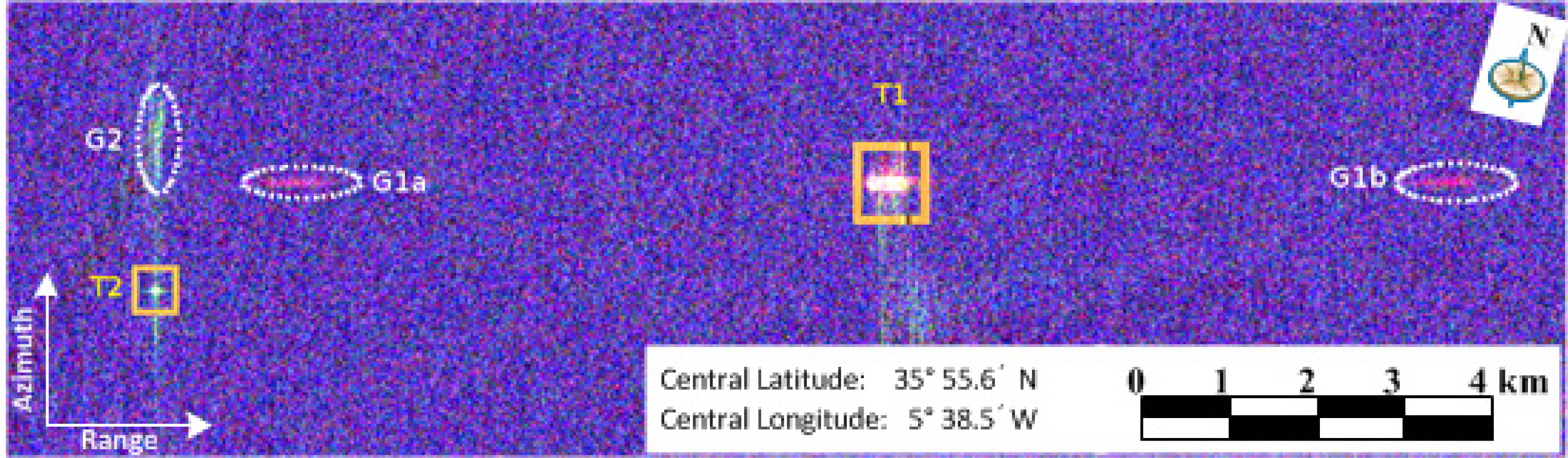
The polarimetric image of Figure 1 with pixel resolution of about 14 m, acquired by RADARSAT-2 sensor over the Gibraltar strait shows two kinds of ghost echoes caused by ships themselves. Ships are denoted by rectangles, whereas ghosts are labeled with dotted ellipses. For the larger ship (T1), two range artifact ghosts (G1a, G1b) can be found on both sides of the ship in the range direction, whereas an azimuth ambiguity over the smaller ship (T2) generates a shifted ghost (G2) in the azimuth direction. According to Equation (1) and the corresponding parameters of the RADARSAT-2 sensor, the estimated shift Δx in azimuth direction between the azimuth ambiguity (G2) and the smaller ship (T2) are approximately 2.8 km, i.e., 200 pixels, while the range shift Δy is about 12 m within one pixel size.
2.2 Polarimetric Analysis of a Complex Scenario
Figure 2a shows a color-coded full-resolution polarimetric SAR image of the sea harbor area of Vancouver city, Canada, onto which some target (T) and ghost (G) focused echoes are indicated. This image indicates that in coastal areas and harbors, man-made structures over sea and land may cause significant range artifact features, like the ghost indicated as G1 caused by the ship labeled T1 or ghosts G2a and G2b resulting from a specific scattering structure noted T2 which is located in the urban area. Moreover, some potentially metallic structures and ships (such as ships T3 and T5) may have highly energetic responses whose side-lobe intensity lies well above the level of reflectivity of the sea. Such artifacts and scattering patterns are susceptible to generate numerous false alarms if classical detection approaches based on contrasts are applied on such a complex data set.
In order to investigate the full-resolution polarimetric behavior of the different elements of the scene under analysis, the polarimetric data are processed through the well-known Cloude-Pottier decomposition technique introduced in [22], and the two most significant parameters of this decomposition are displayed in Figure 2b,c. The entropy, H, represents the degree of randomness of the polarimetric information. H equals 0 for a deterministic response and reaches 1 in case of polarimetric white noise, i.e., for uncorrelated polarimetric channels with equal intensity. The parameter a is an indicator of the nature of the scattering mechanism. A value close to 0 indicates a single bounce reflection, characteristic of scattering by rough surfaces, a = π/4 corresponds to the scattering from anisotropic objects, whereas an a value close to π/2 denotes double-bounce scattering.
The entropy image shown in Figure 2b reveals that for this scene the polarimetric behavior of most of the sea background is highly random, i.e., its polarimetric covariance matrix tends to be isotropic or white, and polarimetrically adaptive detection schemes may have limited performance. Some ships, such as T1, T4, T6, T7, T8, and T9, also have a high degree of polarimetric randomness, due to the mixing of different polarimetric contributions originating from their complex structures as well as from the surrounding sea area and to potentially superimposed artifacts. Due to their high entropy and intermediate a value, they can hardly be discriminated from the surrounding sea. Other ships, such as T3 and T5, with a heading direction perpendicular to the azimuth direction, show a low entropy value and their a parameter reveals the presence of dominant double bounce reflections. This almost deterministic polarimetric behavior, due to a scattering level much higher than the one of their environment, is well adapted to contrast-based detection. Nevertheless, the resulting widespread side-lobes may cause false alarms. One may remark that the ship labeled T1 and its ghost G1 have very similar, very deterministic polarimetric features and hence cannot be discriminated using polarimetric diversity only. In section 5, this extremely perturbed data set is used to demonstrate the performance of the proposed TF analysis method.
3. Principle of Multidimensional Time-Frequency Analysis
3.1. Time-Frequency Analysis Concept
The Time-Frequency decomposition approach used in this work has been proposed for SAR data analysis in [6–9] and is based on the use of a two-dimensional (2D) Short Term Fourier Transform, or 2D Gabor transform. This kind of transformation decomposes a 2D signal, u(l), with l = [x, y] denoting a position in the 2D spatial domain, into different components located around particular spectral coordinates, called sub-spectra, using a convolution with an analyzing function g(l), as follows:
where ω = [ωx, ωy] represents the position in the spectral domain, and u (l0; ω0 ) indicates the decomposition result around the spatial location l0 and frequency location ω0. The application of the Fourier Transform to Equation (2) shows that the spectrum of u (l0; ω0) is given by the following relation:
where U and G indicate signals in the spectral domain. The expressions given in Equation (2) and Equation (3) show that this TF approach can be used to characterize, in the spatial domain, behaviors corresponding to particular spectral components of the signal under analysis. This TF approach being linear and coherent, it is, for adequate spatial and spectral sampling strategies, reversible, i.e., the full resolution original signal u(l) or U(ω) can be reconstructed without loss from a set of samples given by Equation (2). The objective of this TF approach is to analyze spectral properties of the signal around specific spatial locations or equivalently spatial properties around specific spectral locations. Specific spatial spectral components of the signal being selected by the analyzing function g(l), the time and frequency resolutions of the TF analysis are not independent, and their product is fixed by the Heisenberg-Gabor uncertainty relation, given by:
where c is a constant term, determined by the analyzing function g(l). An analyzing function with an excessively narrow bandwidth would involve a high resolution in frequency, but might then lead to a meaningless analysis in the space domain due to a bad localization. Therefore, the expression given in Equation (4) implies a compromise between space and frequency resolutions in order to perform a selective frequency scanning of the signal while maintaining the spatial resolution to values that permit details discrimination.
3.2. SAR Data Time-Frequency Decomposition
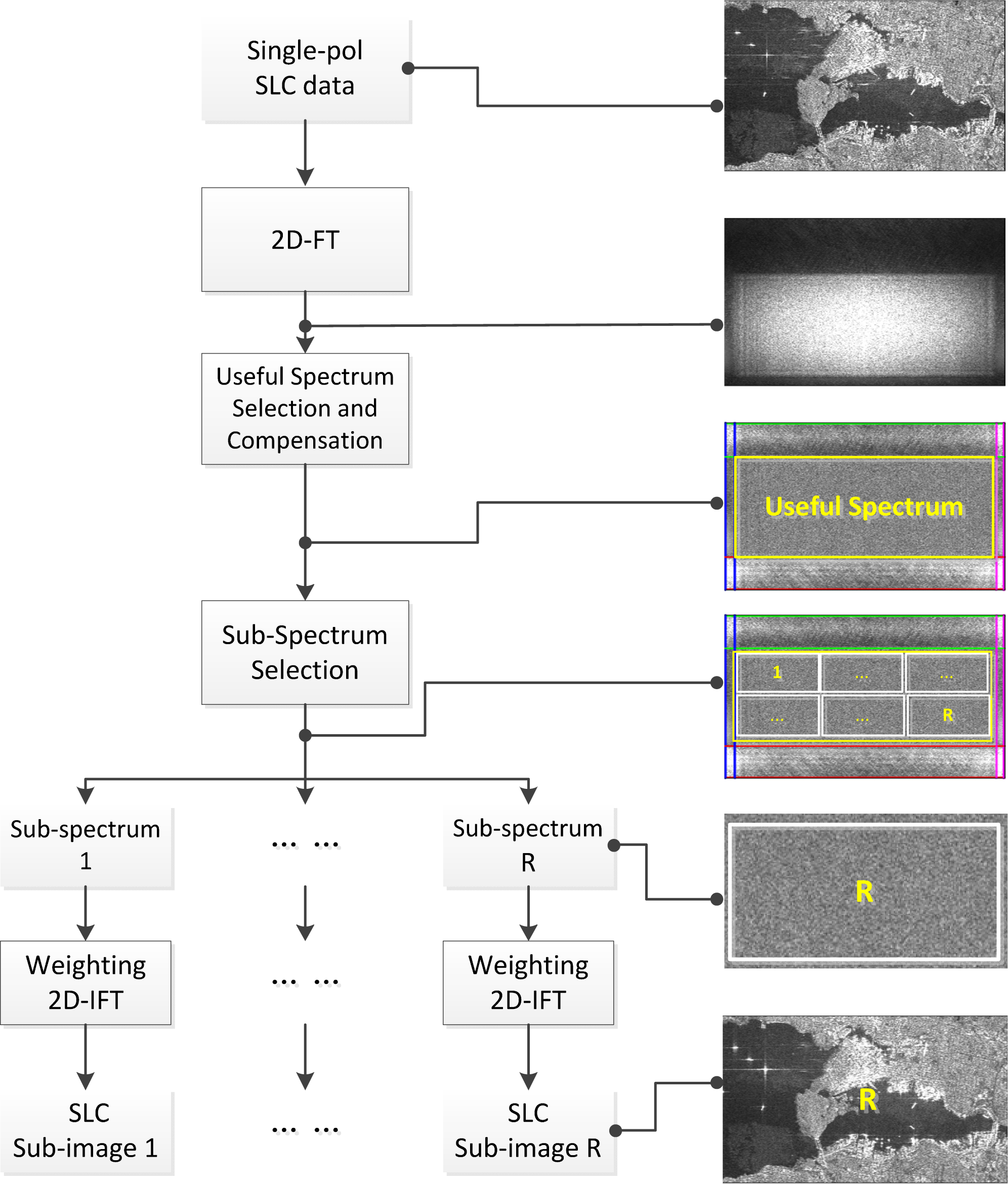
Due to the linearity of SAR focusing, the TF decomposition technique introduced above may either be applied on raw or focused data. Nevertheless, due to the generally limited access to raw data for common end-users and in order to benefit from error corrections and specific signal compensation operated during the focusing of SAR data, TF analysis is usually performed over focused Single-Look Complex (SLC) SAR images. When dealing with coherent SAR images, a 2D spatial location l = [x, y] represents the position of a scatterer in range and azimuth whereas a 2D spectral coordinate ω = [ωx, ωy] corresponds to a specific illumination frequency and azimuthal angle of observation. It is important to note that this interpretation of a spectral location in terms of physical parameters of the SAR acquisition is valid when dealing with coherent SAR data sets and does not hold for incoherent data, like intensity or cross-correlation images. The different steps of the coherent TF decomposition technical details are outlined in Figure 3 in the general 2D case.
- (1)
- 2D Fourier Transform. An SLC SAR image is transformed to the spectral domain using a 2D Fourier Transform (2D-FT).
- (2)
- (3)
- Sub-spectrum selection. The total useful spectrum is divided into R regions, called sub-spectra, centered around specific spectral locations.
- (4)
- Weighting and 2D inverse FT. Each sub-spectrum is then multiplied with a 2D weighting function in order to set the level of the side-lobes of the corresponding SAR impulse-response and is sent back to the spatial domain using a 2D inverse FT (2D-IFT) in order to get an image representing the focused SAR response of the observed scene around a specific spectral location. The set of R sub-images may then be used to characterize some properties of the observed scatterers.
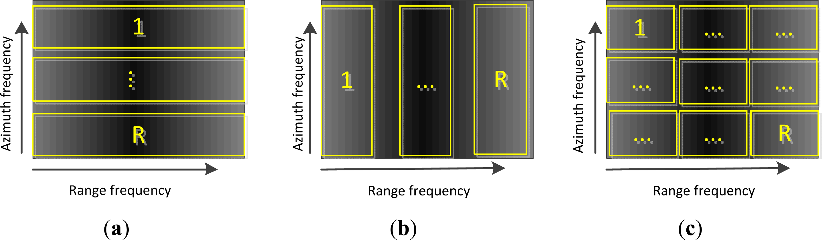
In Figure 4 are illustrated three different decomposition modes corresponding to a TF analysis performed in one dimension, in azimuth or range, or simultaneously in both directions. The ratio between the size of a sub-spectrum and the one of the full available useful spectrum gives, for the considered direction, the loss of spatial resolution inherent to the use of this kind of TF decomposition. In order to easily compare decomposition results obtained around different spectral locations, the R sub-spectra generally have the same size. To preserve a given level of spatial resolution, users might select wider and partly overlapping spectra. As explained below such an approach leads to an artificial correlation of the resulting sub-images, and is generally counterproductive from a statistical point of view.
3.3. Time-Frequency Analysis in the Polarimetric Case
The polarimetric response of a scatterer is fully described, for given acquisition conditions, by its (2 × 2) scattering matrix S, defined in an orthogonal polarization basis, here the Horizontal-Vertical basis, as:
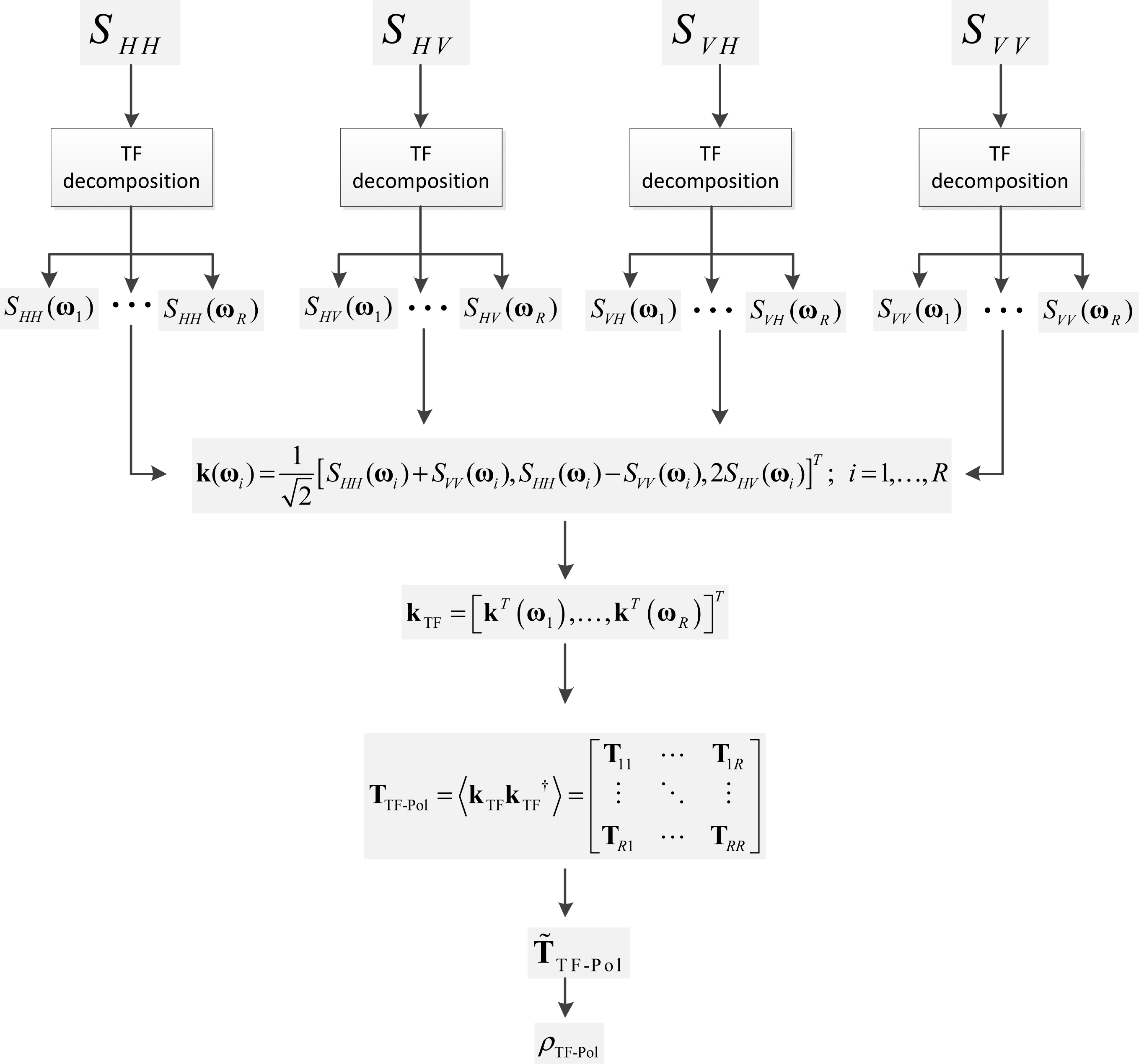
where SPQ represents the complex scattering response of the scatterer, measured over the polarization axis P to an incident wave polarized along direction Q. The TF decomposition summarized in Figure 3 is applied similarly over each of the polarimetric coefficient images and the result is represented, for a given spectral location, by a polarimetric scattering vector, defined as [22,23]:
where ωi represents one of the R spectral locations and T is the transpose operator. The scattering vector given in Equation (6) being obtained from the vectorization of a non-singular linear transformation of the scattering matrix S(ωi), these representations are strictly equivalent. One may note that S(ωi) and k(ωi) have equal Frobenius norms.
4. PolSAR Time-Frequency Analysis
4.1. PolSAR Data TF Model
The discrimination of ships from their environment is implemented in this work as the detection of artificial, i.e., man-made objects, lying in a natural background using a multi-component TF signal model proposed in [8,9]:
where ω represents a location in the spectral domain whereas its spatial counterpart, l, is omitted to simplify the expressions. The signal u(ω) represents a polarimetric scattering vector, defined in Equation (6), sampled around a given spectral position and modeled as the sum of three contributions:
- The term t(ω) represents the response of an artificial scatterer having deterministic or almost deterministic scattering patterns. As a consequence this contribution is highly coherent, i.e., presents a high-level of correlation between samples taken at different spectral locations. Depending on the structure of the observed target, this component can remain constant during the SAR acquisition, or can be non-stationary if the backscattering behavior is sensitive to the azimuth angle of observation or illumination frequency.
- The second term c(ω) represents the response of natural distributed environments, or clutter, largely affected by the speckle effect. This contribution is incoherent, i.e., samples corresponding to non-overlapping spectra are uncorrelated, and may show a non-stationary behavior in particular cases.
- The last term n(ω) corresponds to the acquisition noise, assumed to be stationary and incoherent.
The studies led in [8,9] proposed to characterize the total TF response, u(ω), by studying its stationarity and coherence over the whole spectral domain, through second-order statistics. In the case of SAR signals acquired by space-borne sensors, characterized by a small frequency bandwidth and a very small azimuthal aperture, investigating the non-stationary behavior of the scene’s response might be misleading, since potential variations of the signal might be due to processing artifacts instead of being related to physical scattering effects. The coherence of u(ω) can be used to determine the dominant component within the pixel under consideration: a high coherence value of u(ω) indicates that t(ω) is the most important term in Equation (7), whereas a low one corresponds to scattering from an incoherent and distributed medium or to a response dominated by the acquisition noise.
4.2. Second Order Statistics
In order to study second-order TF polarimetric statistics, a 3R element TF scattering vector is defined by gathering the information sampled at different spectral locations as follows:
Thereby, a polarimetric TF coherency 3R × 3R matrix, ∑TF-Pol, is built as follows [7]:
where E(·) denotes the expectation operator, ∑ij = E(k(ωi)k(ωj) †)i,j=1,…,R, and † corresponds to the transpose conjugate operator. The 3 × 3 ∑ii matrices, with i = 1,…, R, represent polarimetric coherency matrices at the R spectral locations, whereas ∑ij, with i ≠ j, correspond to spectral cross-correlation terms.
4.3. Polarimetric TF Coherence Indicator
Coherence is assessed by testing the level of cross-correlation between the signals sampled around different spectral locations. In the multivariate polarimetric case, this test is performed by considering the hypothesis of total uncorrelation [9]:
This hypothesis is then tested by considering that, under the usual assumption of normally distributed SLC data, the ni-look Maximum Likelihood (ML) estimate of ∑TF-Pol, i.e.,
, follows a Wishart distribution TTF-Pol ∼ W (ni, ∑TF-Pol). The ML ratio used to test the hypothesis H0 is given by [9]:
where Tii represent the ni-look ML estimate of ∑ii.
This ML ratio expression can be rewritten as [9]:
with T̃TF-Pol, a normalized TF coherency matrix defined as:
where
, with
. The normalized coherency matrix, T̃TF-Pol, results from the whitening of the TF polarimetric coherency matrix TTF-Pol by the separate polarimetric information at each spectral location. This formulation of the ML ratio using normalized polairmetric quantities demonstrates the robustness of the test to variations of the backscattered intensity or polarimetric scattering patterns, and its independence with respect to potential non-stationary behaviors. The normalized off-diagonal matrices Γij can be viewed as an extension of the scalar normalized correlation coefficient to the polarimetric case. From the ML ratio expression given in Equation (13) is defined a correlation indicator, named polarimetric TF coherence, as [9]:
The value of polarimetric TF coherence indicator ρTF-Pol lies between 0, in the decorrelated case where T̃TF-Pol → Id and 1, when the tested hypothesis is not true, i.e., |T̃TF-Pol| → 0. The indicator ρTF-Pol reaches high values over coherent reflectors whose contribution dominates the global responses, such as man-made targets, ships and buildings, etc. In contrast, a low value of ρTF-Pol corresponds to natural environments like ocean, sea, forest, vegetation area, etc. It is important to note that ρTF-Pol is independent of the backscattered intensity, i.e., it should show similar values over forested areas, generally having a highly energetic response and over sea, known to show a much lower level of reflectivity. In order to guarantee an optimal level of efficiency to this ML ratio test approach, the TF sampling strategy used to build the TF coherency should follow the recommendations summarized in Figure 4, i.e., the different sub-spectra should not overlap. Indeed, in case of overlapping spectra, the clutter responses sampled at different spectral locations would be artificially correlated, ρTF-Pol would be biased towards 1, and the global artificial objects detection approach would be less efficient, due to a poorer contrast between natural environments and artificial objects. The PolSAR TF coherence calculation procedure is illustrated by a flowchart displayed in Figure 5.
4.4. Polarimetric TF Coherent Scattering Mechanism Indicator
The proposed PolSAR TF coherence analysis techniques can also be used to further characterize the polarimetric scattering patterns of coherent scatterers, i.e., of the detected targets. As proposed in [9], the first eigenvector of T̃TF-Pol, named υ1, and corresponding to the most coherent polarimetric TF scattering behavior, can be transformed back to the H-V polarimetric basis using a matrix block-diagonal P, satisfying T̃TF-Pol = PTTF-PolP†. Selecting and normalizing the first three elements of the transformed eigenvector, one gets a unitary scattering vector υopt which can be characterized using the parametric expression given by [22]:
In particular, the new parameter αTF, describing the nature of the most coherent scattering pattern over a target, was shown to deliver more contrasted and relevant information than the original full resolution parameter α [9].
Compared with the previous work [8,9], the technical novelties in this work can be summarized:
- The performance of different TF analysis modes, i.e., in separate azimuth and range directions and in both directions, rather than in only azimuth direction [12,14,15,17], are assessed for different sea scenario. The proposed technique is shown to perform well when applied, in separate azimuth and range directions, or over both axis, onto coarse-resolution space-borne data, whereas preceding TF studies [7,13,16] concentrated on a single direction or used finer resolution airborne SAR images. This aspect is particularly important since it demonstrates the applicability of the technique over a wider range of SAR images, including data sets acquired by space-borne sensors.
5. Experimental Analysis and Discussions
In this section, the proposed polarimetric TF analysis technique is applied to the discrimination of ships in complex scenes, involving severe ambiguity or processing artifact related ghost echoes as well as small emerged lands, using experimental fully polarimetric data set composed of three Fine-Quad (FQ) mode RADARSAT-2 images over the scenes of Vancouver, Canada, (FQ15, two images) and San Francisco, USA, (FQ9). The choice of a TF decomposition mode is assessed from the performance of the polarimetric TF coherence indicator ρTF-Pol for ship discrimination in open sea area in the presence of strong ghost echoes and some natural islands.
5.1. Sea Environment in the Presence of Ghost Echoes
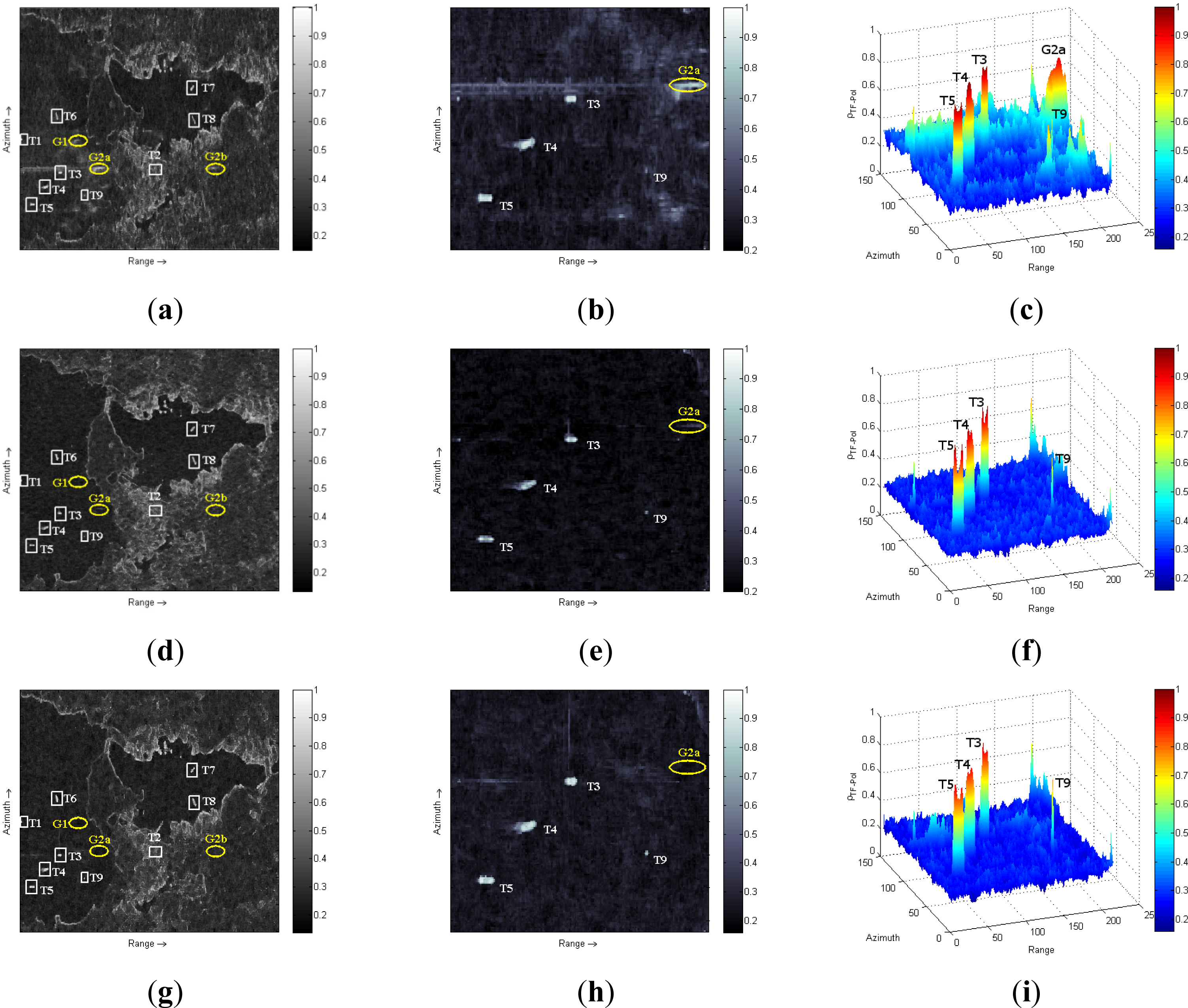
The polarimetric TF coherence analysis is applied to the Vancouver harbor data set presented in Figure 2 for a spectral sampling performed in azimuth or range direction only and in both directions. The corresponding TF coherence maps are given in Figure 6.
The top row of Figure 6 displays coherence results obtained using a TF decomposition in the azimuth direction at four spectral locations. Each azimuth sub-spectrum occupies 25% of the total available azimuth spectrum, as shown in Figure 4a. The middle row of Figure 6 shows results obtained using a similar analysis in the range direction, with 4 range sub-spectra occupying each 25% of the whole available range spectrum, as shown in Figure 4b. The bottom row presents ρTF-Pol maps obtained using 4 sub-spectra sampled over both azimuth and range directions, with two frequency locations in each direction, each sub-spectrum occupying 25% of the total available 2D spectrum, as shown in Figure 4c.
Compared with the full-resolution polarimetric features depicted in Figure 2, the ρTF-Pol maps displayed in Figure 6 show the power of discrimination of the proposed TF analysis technique for ship discrimination in severe backgrounds, especially for the ships T1, T4, T6, T7, and T8 which are mixed with different polarimetric contributions originating from their complex structures as well as from the surrounding sea area, as seen from Figure 2b,c. Distributed environments like the sea and continental ground have small TF coherence values, whereas ships are recognized as highly coherent scatterers. Moreover, these results indicate that this approach can effectively mitigate artifacts related to SAR ambiguity, as widespread ghosts with high entropy are filtered out due to their incoherent behaviors and point-like ones, such as ghosts G1 and G2a, shown in Figure 6d,g, which could have easily been misinterpreted as ships by conventional discrimination techniques, have been cancelled too. Over this particular scene shown in Figure 6a–c, the azimuth-only TF mode is less efficient than the range-only one, as it cannot completely cancel the range artifacts (G1 and G2a) and shows a smaller contrast between artificial and natural scatters. One may note that this technique can reduce cross-shaped side-lobes generated by the ships T3 and T5, which could have been also misclassified as targets. In addition, as shown in Figure 6a,d,g, besides the larger ships (T3–T8), the smaller ship (T9) can be detected and localized, despite the fact that TF analysis techniques may degrade the spatial resolution. Therefore, the proposed ρTF-Pol indicator permits to detect ships, even though the sea environment is complex due to ghost echoes and highly random polarimetric behavior of the scene shown in Figure 2.
In order to quantitatively measure the target-to-clutter contrast of the proposed TF indicator, mean values and standard deviations of the polarimetric TF coherence ρTF-Pol value are computed over ships (targets), overs their surrounding sea background (clutter), and over ghost echo responses (ghosts). Every region was delineated by manual segmentation. As shown in Figure 7, in the azimuth-only decomposition mode, ghost responses remain coherent, whereas the other two decomposition modes permit to reduce ghost responses to the clutter level. This aspect reveals that the introduction of range TF diversity can remove ghost echoes related to range artifacts. However, in the range-only decomposition mode, all the ships show a lower coherence value compared to the results obtained in azimuth-only and in the 2D case. This difference is due to the much better resolution of the original data set in the azimuth direction: the loss of resolution inherent to the use of a TF analysis is less critical in the azimuth direction where more refined target details can be preserved. Among all three decomposition modes, the 2D TF decomposition approach performs best, with a high contrast between targets and clutters and important ghost filtering capabilities. In this particular scene perturbed by range artifacts, the range-only mode possesses the advantage of less processing complexity and computation time than the 2D TF mode, because the 1D mode is easier to implement in the decomposition step.
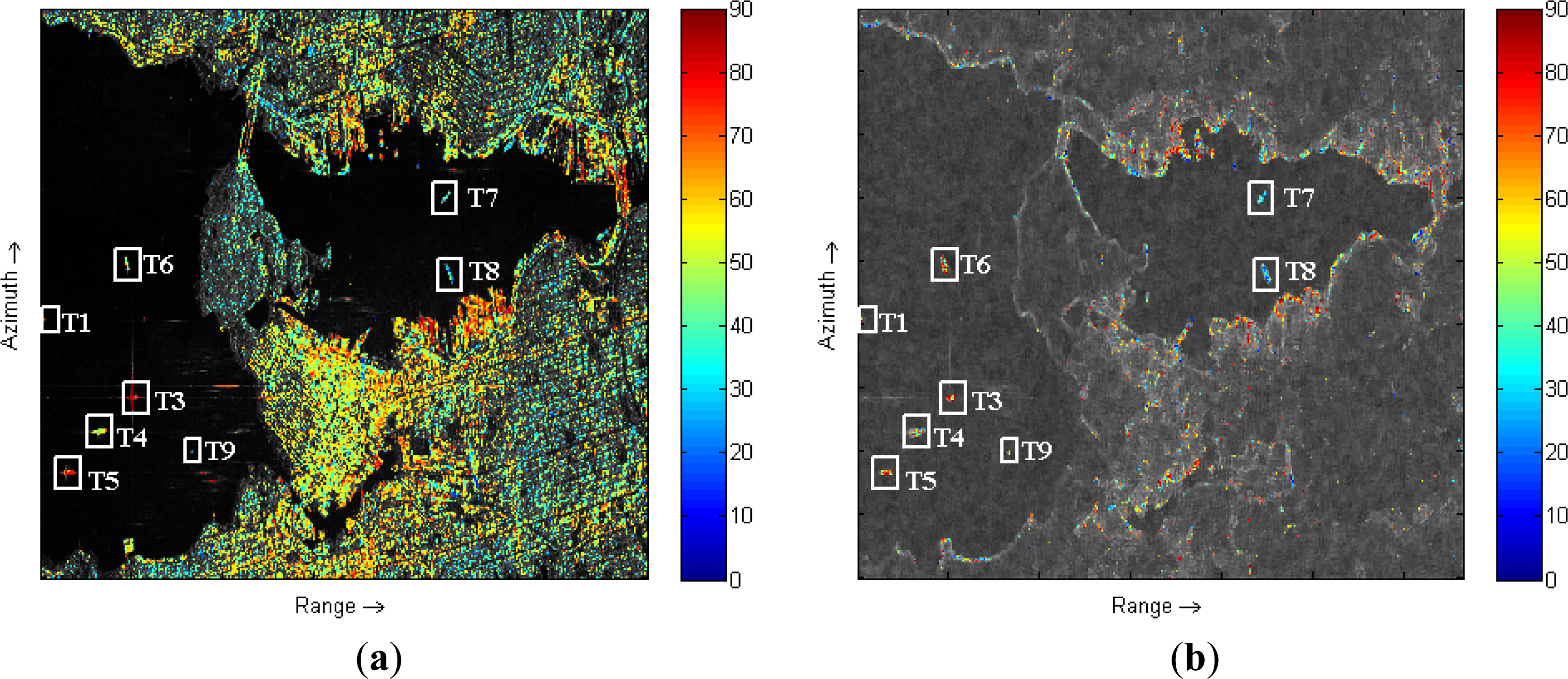
The full-resolution polarimetric α of the objects with strong backscattering intensity is presented in Figure 8a. The proposed new TF polarimetric parameter αTF is extracted over every target verifying ρTF-Pol > 0.7, and displayed in Figure 8b. Comparing the ships in Figure 8a,b, we can see different polarimetric behaviors of the same ship. For example, in Figure 8a the ship T6 is with inter-mediate α, but in Figure 8b it contains more components dominated by double bounce reflections, i.e., their αTF values are close to π/2. The ship T9 shows single bounce reflection in Figure 8a, while it has higher αTF value in Figure 8b. It is more reasonable to use the αTF parameter to characterize ships, because the ships should consist of many double bounce reflectors. Nevertheless, the results over the Vancouver harbor area indicate that the proposed TF approach can be used as a filter that cleans the original perturbed full-resolution image in order to emphasize and better describe coherent scattering behaviors.
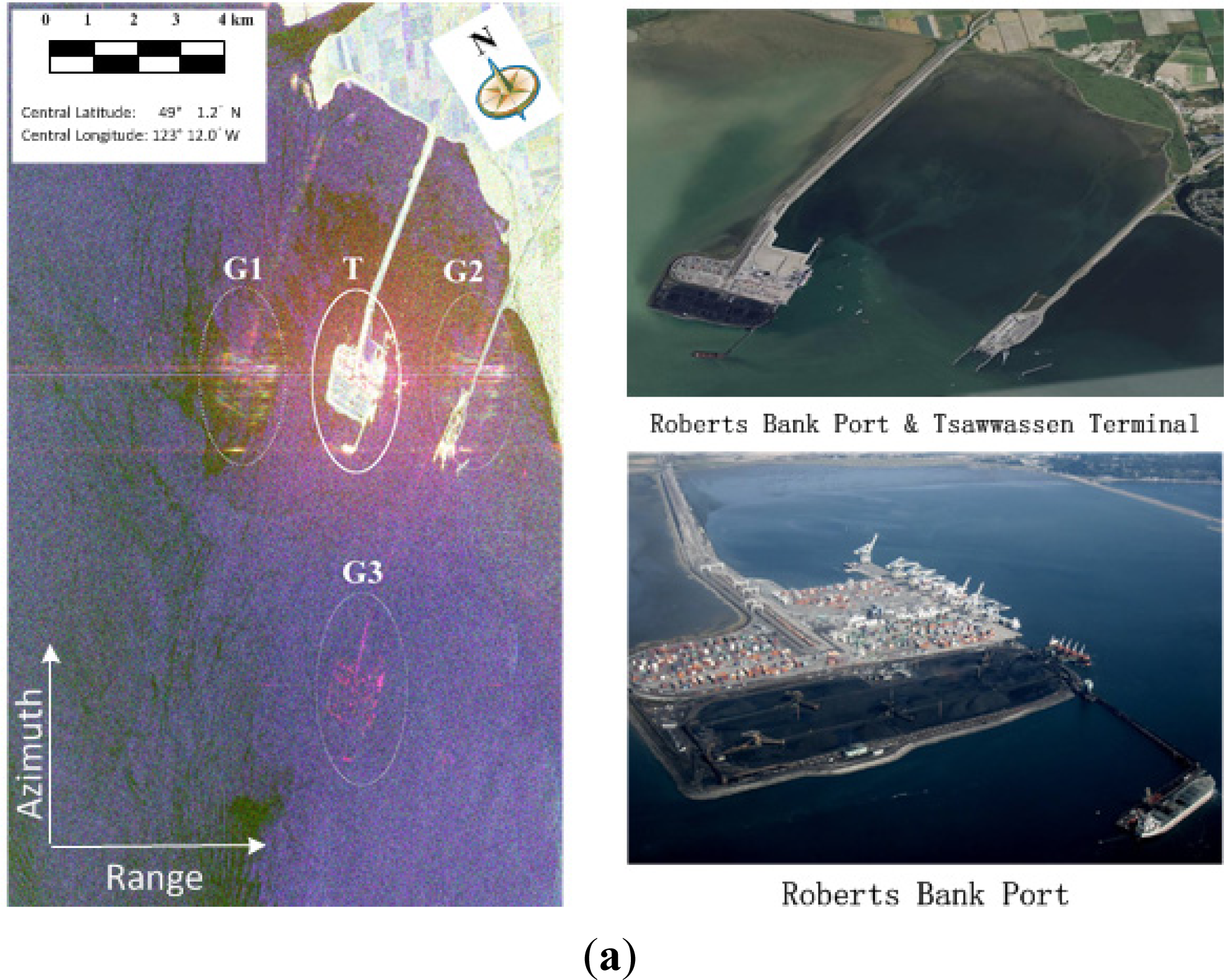
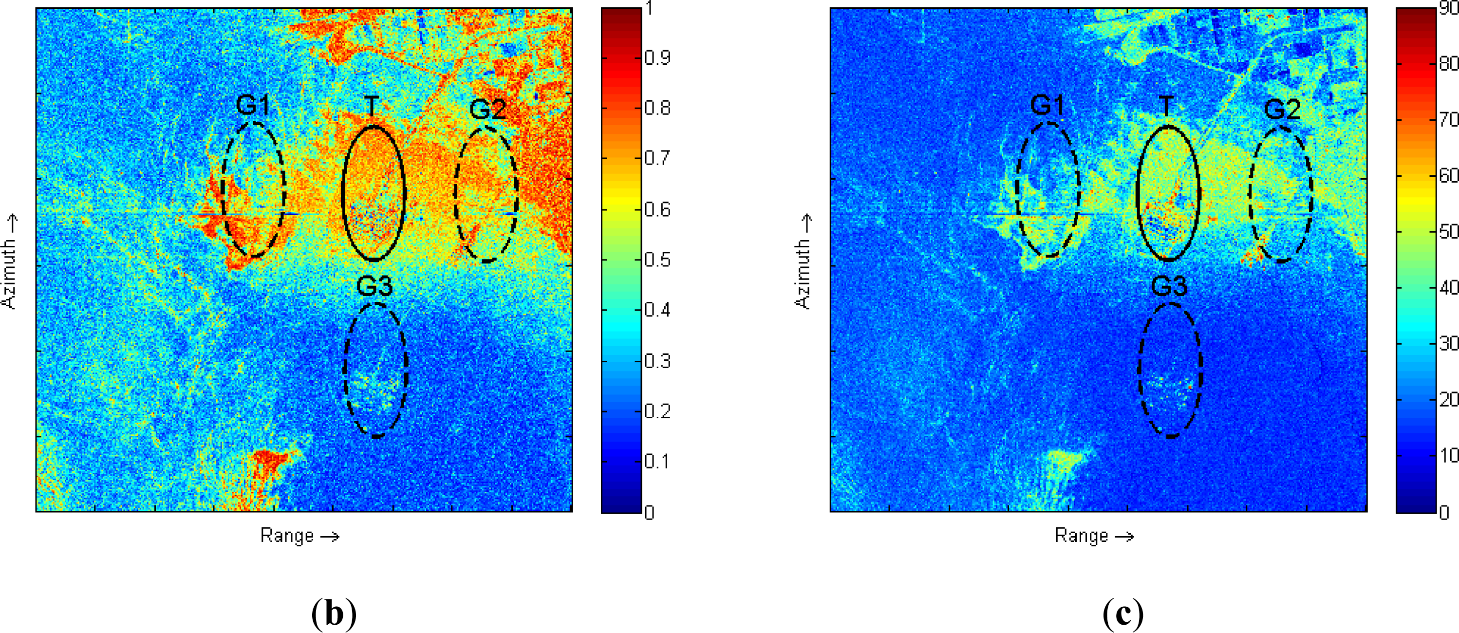
Another scene, affected by strong ghost echoes generated from a coal and container port, is shown in Figure 9a. The port called “Roberts Bank” is located at Georgia Strait in the Vancouver sea area near the border between Canada and USA. The “Roberts Bank” port (T) denoted by a solid white ellipse, causes two range artifacts (G1, G2) and an azimuth ambiguity (G3). These kinds of ghosts can be easily mistaken as real targets and lead to serious false alarms in terms of ship detection. The full-resolution polarimetric entropy H and α images displayed in Figure 9b,c, indicate that classical polarimetric detectors would meet some problems over this kind of scene.
The Roberts Bank port area is analyzed for the same TF modes used in Figure 6. Figure 10a,b shows that the ships (T1 and T2) have high ρTF-Pol values, but the range ghost G1 is also highly coherent. The range ghost area G1 is well suppressed when the TF decomposition includes the range direction too, as seen in Figure 10c–f. The 2D TF decomposition mode permits to filter range and azimuth ghosts, while preserving a high level of coherence over ships.
5.2. Sea Environment with Presence of Small Natural Islands
Classical automatic ship detection strategies require to mask out small islands in order to avoid confusing these emerged lands with ships, based on their high contrast with sea. Here, natural islands are defined as uninhabited islands without man-made objects, and may be covered with some vegetation. Due to its ability to separate man-made structures from natural background, the proposed polarimetric TF coherence is expected to avoid false alarms over such environments. The TF analysis is run over a RADARSAT-2 data set acquired in Fine Quad-Pol mode (FQ9) over the San Francisco area, USA. Figure 11a,b show an optical image and a polarimetric color-coded Pauli basis image of this area. It should be noted that the optical image used here as a coarse reference, was not acquired at the same time as the SAR image. As shown in Figure 11b, some ships (marked by yellow solid rectangles) may be observed in the sea area. Some ghost echoes (G1, G2 denoted in white ellipses) caused by ships and other man-made structures can be observed too. As mentioned in Section 5.1, the TF analysis mode operation in both directions has the best performance for ghost removal and target detail preservation. Therefore, this mode is used for analyzing this data set and the results displayed in Figure 11c, show that all the ships denoted by yellow rectangles can be detected, and the ghost echoes (in G1, G2 area) are efficiently removed.
Two islands, indicated by white rectangles, can be seen on the images: the smaller one (i1) in the top-left part of the image, called “Red Rock” island (see i1 optical image at the right side of Figure 11a), is an uninhabited 5.8-acre (2.3 ha) emerged island in the San Francisco Bay located just South of the Richmond-San Rafael Bridge. This “Red Rock” island can be considered as a natural island. The larger one (i2) in the middle part of the image is the “Alcatraz island”, and is equipped with facilities and landmarks such as lighthouse, some buildings, etc.
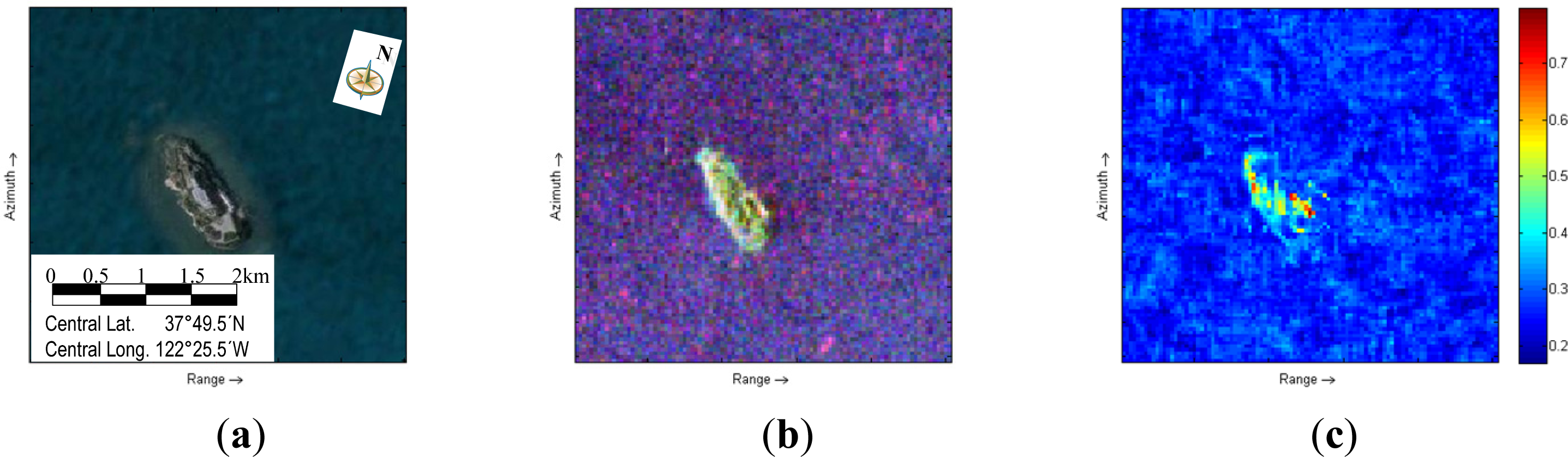
Figure 12 contains the results obtained over the Red Rock island (i1) area which also includes a part of the Richmond-San Rafael Bridge, a ship (T1) near the Chevron tanker terminal, etc. Figure 13 concentrates on the Alcatraz island area. Comparing both figures, one finds that the “Red Rock” island is filtered out of the ρTF-Pol image as the natural environments it contains have an incoherent response, fully dominated by speckle, whereas over the Alcatraz island, coherent scatterers related to complex man-made targets can be detected. Therefore, the proposed approach cannot be used to differentiate ships from other coherent objects in the sea, like inhabited islands, oil rigs and other man-made targets. Other advanced techniques should be investigated to resolve this problem. Nevertheless, this study shows that the proposed polarimetric TF indicator can be efficiently used against false alarms generated by small emerged and uninhabited lands which may be not indicated on coarse cartographic maps.
6. Conclusions
In this paper, a new full polarimetric Time-Frequency coherence and polarimetrically adaptive indicator has been introduced to address the problems of ship discrimination over complex sea environments. A multi-component PolSAR TF signal model has been developed and applied to derive a full polarimetric TF coherent descriptor. This polarimetric TF coherence descriptor was used for ship discrimination in different complex backgrounds, including azimuth ambiguities, range artifacts, and small natural islands. Results showed that ships could be detected due to their highly coherent scattering characteristic, whereas ghost echoes and distributed area were suppressed due to their lower coherence value. In addition, three TF decomposition modes with different analysis directions, i.e., along separate azimuth or range axis or simultaneously in both directions, have been compared and evaluated. It was found that the 2D TF decomposition mode performed best in terms of ghost echoes removal, and permitted to preserve a high level of coherence and details over ships. Moreover, polarimetric indicators extracted from the detected ships or other man-made targets, have been shown to provide more information than the full resolution original ones. This suggests more possibilities of enhanced ship discrimination in other more complex sea scenarios where full resolution polarization does not perform well. Future studies will address the ship discrimination using TF coherence analysis with dual or compact polarization mode and combined with other multidimensional SAR processing techniques.
Acknowledgments
The reviewers’ constructive comments to improve the paper are greatly appreciated. This work was supported in part by China Scholarship Council grant (No. 2011611070) and also by the National Natural Science Foundation of China under Grant 61201338.
Conflict of Interest
The authors declare no conflict of interest.
References
- Nunziata, F.; Migliaccio, M.; Brown, C.E. Reflection symmetry for polarimetric observation of man-made metallic targets at sea. IEEE J. Ocean. Eng 2012, 37, 384–394. [Google Scholar]
- Nunziata, F.; Migliaccio, M. On the cosmo-skymed pingpong mode to observe metallic targets at sea. IEEE J. Ocean. Eng 2013, 38, 71–79. [Google Scholar]
- Velotto, D.; Nunziata, F.; Migliaccio, M.; Lehner, S. Dual-polarimetric terrasar-x SAR data for target at sea observation. IEEE Geosci. Remote Sens. Lett 2013, 10, 1114–1118. [Google Scholar]
- Marino, A. A notch filter for ship detection with polarimetric sar data. IEEE J. Sel. Top. Appl. Earth Obs. Remote Sens 2013, 6, 1219–1232. [Google Scholar]
- Wang, N.; Shi, G.; Liu, L.; Zhao, L.; Kuang, G. Polarimetric sar target detection using the reflection symmetry. IEEE Geosci. Remote Sens. Lett 2012, 9, 1104–1108. [Google Scholar]
- Ferro-Famil, L.; Reigber, A.; Pottier, E.; Boerner, W.-M. Scene characterization using subaperture polarimetric SAR data. IEEE Trans. Geosci. Remote Sens 2003, 41, 2264–2276. [Google Scholar]
- Ferro-Famil, L.; Reigber, A.; Pottier, E. Nonstationary nutural media analysis from polarimetric sar data using a two-dimensional time-frequency decompostion approach. Can. J. Remote Sens 2005, 31, 21–29. [Google Scholar]
- Ferro-Famil, L.; Leducq, P.; Reigber, A.; Pottier, E. Extraction of information from the Time-Frequency Polinsar Response of Anisotropic Scatterers. Proceedings of 2005 IEEE International Geoscience and Remote Sensing Symposium, Seoul, Korea, 25–29 July 2005; pp. 4856–4859.
- Ferro-Famil, L.; Pottier, E. Urban Area Remote Sensing from l-Band Polsar Data Using Time-Frequency Techniques. Proceedings of IEEE Urban Remote Sensing Joint Event, Paris, France, 11–13 April 2007; pp. 5045–5048.
- Sauer, S.; Ferro-Famil, L.; Reigber, A.; Pottier, E. Three-dimensional imaging and scattering mechanism estimation over urban scenes using dual-baseline polarimetric insar observations at l-band. IEEE Trans. Geosci. Remote Sens 2011, 49, 4616–4629. [Google Scholar]
- Huang, Y.; Ferro-Famil, L.; Reigber, A. Under-foliage object imaging using sar tomography and polarimetric spectral estimators. IEEE Trans. Geosci. Remote Sens 2012, 50, 2213–2225. [Google Scholar]
- Arnaud, A. Ship Detection by SAR Interferometry. Proceedings of 1999 IEEE International Geoscience and Remote Sensing Symposium, Hamburg, Germany, 28 June–2 July 1999; pp. 2616–2618.
- Souyris, J.-C.; Henry, C.; Adragna, F. On the use of complex SAR image spectral analysis for target detection: Assessment of polarimetry. IEEE Trans. Geosci. Remote Sens 2003, 41, 2725–2734. [Google Scholar]
- Ouchi, K.; Tamaki, S.; Yaguchi, H.; Iehara, M. Ship detection based on coherence images derived from cross correlation of multilook SAR images. IEEE Geosci. Remote Sens. Lett 2004, 1, 184–187. [Google Scholar]
- Ouchi, K.; Wang, H. Interlook cross-correlation function of speckle in SAR images of sea surface processed with partially overlapped subapertures. IEEE Trans. Geosci. Remote Sens 2005, 43, 695–701. [Google Scholar]
- Schneider, R.Z.; Papathanassiou, K.P.; Hajnsek, I.; Moreira, A. Polarimetric and interferometric characterization of coherent scatterers in urban areas. IEEE Trans. Geosci. Remote Sens 2006, 44, 971–984. [Google Scholar]
- Brekke, C.; Anfinsen, S.N.; Larsen, Y. Subband extraction strategies in ship detection with the subaperture cross-correlation magnitude. IEEE Geosci. Remote Sens. Lett 2013, 10, 786–790. [Google Scholar]
- Liu, C.; Gierull, C.H. A new application for polsar imagery in the field of moving target indicator/ship detection. IEEE Trans. Geosci. Remote Sens 2007, 45, 3426–3436. [Google Scholar]
- Velotto, D.; Soccorsi, M.; Lehner, S. Azimuth ambiguities removal for ship detection using full polarimetric X-band SAR data. IEEE Trans. Geosci. Remote Sens 2013, 52, 76–88. [Google Scholar]
- Liu, C.; Vachon, P.W.; English, R.A.; Sandirasegaram, N. Ship Detection Using Radarsat-2 Fine Quad Mode and Simulated Compact Polarimetry Data; Defence R&D Canada: Ottawa, ON, Canda, 2010. [Google Scholar]
- Raney, R.K.; Princz, G.J. Reconsideration of azimuth ambiguities in SAR. IEEE Trans. Geosci. Remote Sens. 1987, GE-25, 783–787. [Google Scholar]
- Cloude, S.R.; Pottier, E. An entropy based classification scheme for land application of polarimetric SAR. IEEE Trans. Geosci. Remote Sens 1997, 35, 68–78. [Google Scholar]
- Cloude, S.R.; Pottier, E. A review of target decomposition theorems in radar polarimetry. IEEE Trans. Geosci. Remote Sens 1996, 34, 498–518. [Google Scholar]
Figure 1.
Color-coded Pauli basis image (
HH + VV,
HV + VH,
HH – VV) of the polarimetric data acquired by the RADARSAT-2 sensor over the strait of Gibraltar.
Figure 1.
Color-coded Pauli basis image (
HH + VV,
HV + VH,
HH – VV) of the polarimetric data acquired by the RADARSAT-2 sensor over the strait of Gibraltar.

Figure 2.
Full resolution polarimetric features of a RADARSAT-2 image acquired over the Vancouver harbor area (Canada). (a) Polarimetric color-coded image (
HH + VV,
HV + VH,
HH – VV). (b) polarimetric entropy H. (c) polarimetric a angle. Some ships Ti and ghosts Gi are indicated by rectangles and ellipses, respectively.
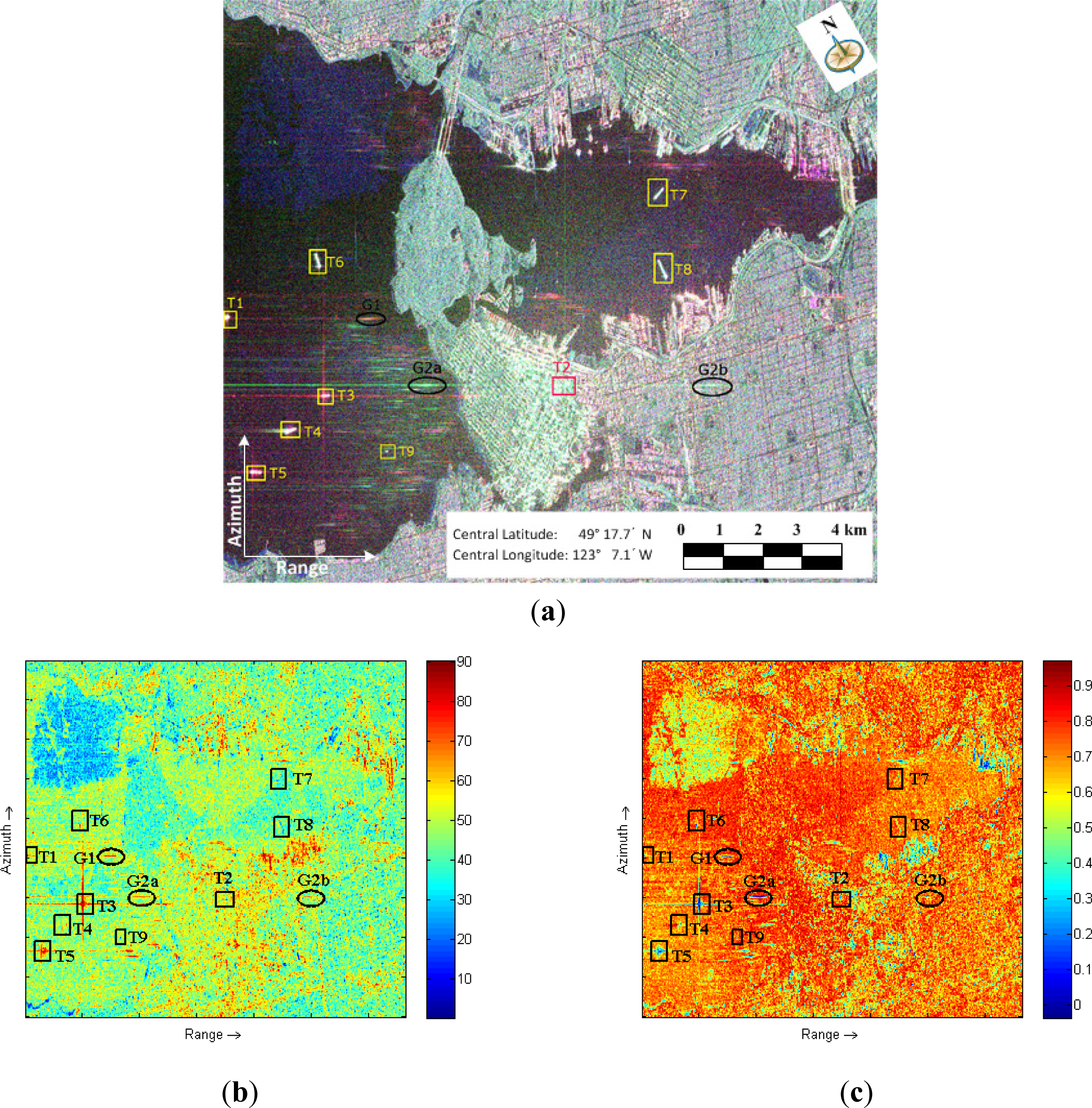
Figure 3.
Flow chart of the TF decomposition approach.

Figure 4.
Illustration of three decomposition modes of a 2D spectrum. Decomposition (a) in azimuth direction only with a range resolution kept to its original value. (b) in range direction only with a unaffected azimuth resolution. (c) in both directions.
Figure 4.
Illustration of three decomposition modes of a 2D spectrum. Decomposition (a) in azimuth direction only with a range resolution kept to its original value. (b) in range direction only with a unaffected azimuth resolution. (c) in both directions.

Figure 5.
Flowchart of PolSAR coherence TF analysis.

Figure 6.
Polarimetric TF coherence ρTF-Pol evaluated over the Vancouver harbor data set with different TF modes: (az) in the azimuth direction only, (rg) in the range direction only (az & rg) in both directions simultaneously. (a) ρTF-Pol (az). (b) Closeup of ρTF-Pol (az). (c) 3D view of ρTF-Pol (az) in (b). (d) ρTF-Pol (rg). (e) Closeup of ρTF-Pol (rg). (f) 3D view of ρTF-Pol (rg) in (e), (g) ρTF-Pol (az&rg). (h) Closeup of ρTF-Pol (az&rg). (i) 3D view of ρTF-Pol (az&rg) in (h).

Figure 7.
Comparison of ρTF-Pol coherence values obtained with three TF decomposition modes over the Vancouver harbor area. Error bars indicate standard deviations computed over the areas indicated in Figure 6.
Figure 7.
Comparison of ρTF-Pol coherence values obtained with three TF decomposition modes over the Vancouver harbor area. Error bars indicate standard deviations computed over the areas indicated in Figure 6.
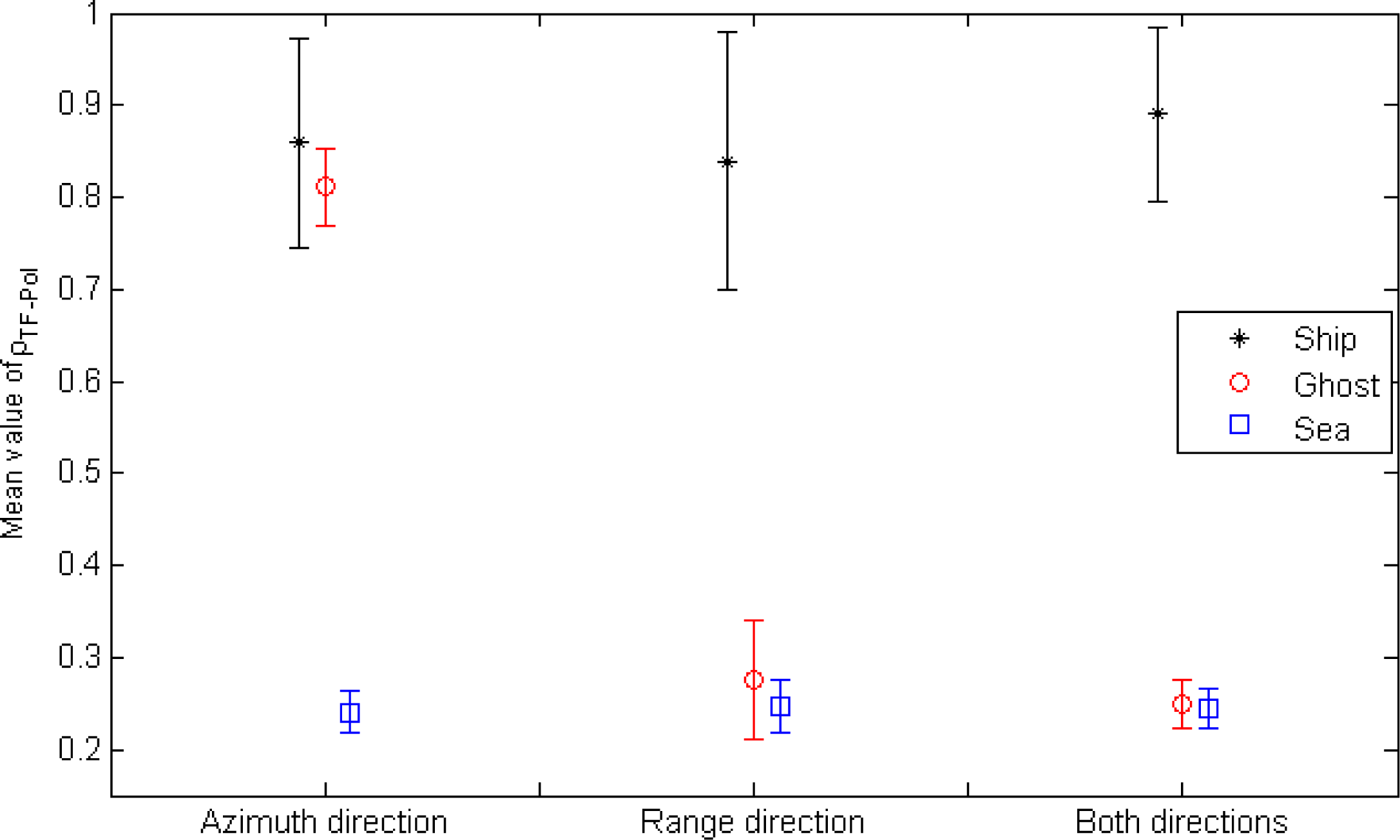
Figure 8.
Images of the Vancouver harbor area. (a) Full-resolution polarimetric α value of ships and other objects with strong backscattering intensity, superimposed on the SPAN image (SPAN = |SHH|2 + |SHV|2 + |SVH|2 + |SVV|2). (b) TF polarimetric αTF result over coherent scatterers. The corresponding αTF results are superimposed on the ρTF-Pol image obtained with a TF decomposition performed in both directions shown in Figure 6g.

Figure 9.
Polarimetric features of the RADARSAT-2 data set acquired over “Roberts Bank” port in Vancouver near the border between Canada and USA. (a) (Left): Color-coded Pauli image (Right): Optical image of the “Roberts Bank” port and “Tsawwassen Ferry Terminal”. (b) Full-resolution polarimetric entropy H image. (c) Full-resolution polarimetric α image. The port is indicated using a solid line ellipse, whereas ghosts are outlined by dotted ellipses.


Figure 10.
Polarimetric TF coherence ρTF-Pol computed over Roberts Bank port area data set with different TF modes: (az) in the azimuth direction only, (rg) in the range direction only (az & rg) in both directions simultaneously. Two small ships (T1 and T2) are outlined by rectangles. (a) ρTF-Pol(az), (b) 3D view of ρTF-Pol(az) details, (c) ρTF-Pol(rg), (d) 3D view of ρTF-Pol(rg) details, (e) ρTF-Pol(az & rg), (f) 3D view of ρTF-Pol(az & rg) details.


Figure 11.
Images of San Francisco area. Ships: yellow rectangles; Islands (i1, i2): white rectangles; Ghost echoes (G1,G2): white ellipses. (a) Left: Optical images. Right: Island i1, named “Red Rock”, is an uninhabited, 5.8-acre island; Island i2, called “Alcatraz island”, has man-made targets and covers 22 acres. (b) Pauli image from RADARSAT-2 data. (c) ρTF-Pol image with TF decomposition in both directions.
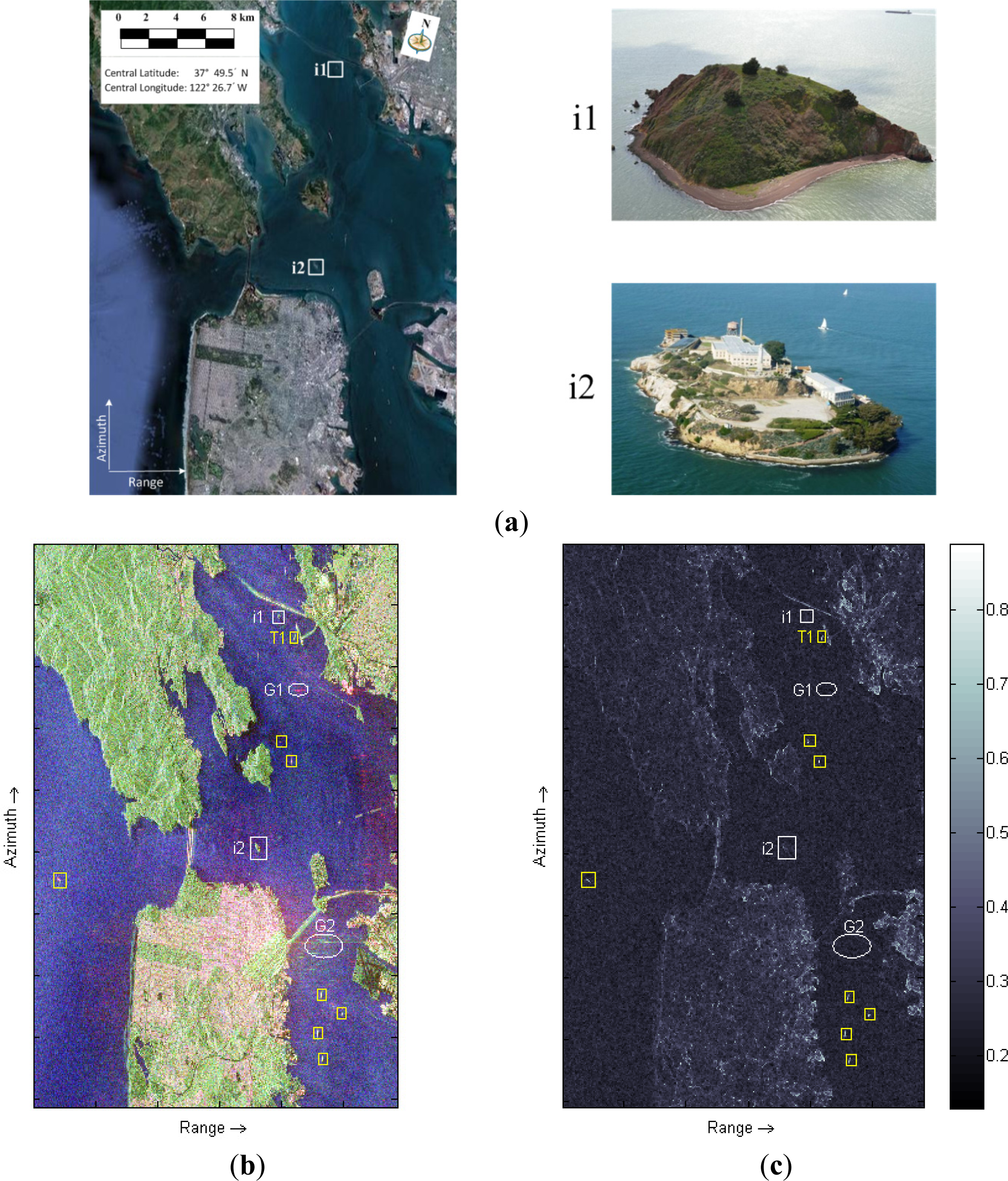
Figure 12.
Red Rock island area. Ship T1 denoted in yellow rectangle is near the Chevron tanker terminal shown in the bottom-right corner of the image; “Red Rock”, is outlined by dashed white rectangle. (a) Optical image. (b) Pauli image. (c) ρTF-Pol image.
Figure 12.
Red Rock island area. Ship T1 denoted in yellow rectangle is near the Chevron tanker terminal shown in the bottom-right corner of the image; “Red Rock”, is outlined by dashed white rectangle. (a) Optical image. (b) Pauli image. (c) ρTF-Pol image.

Figure 13.
Alcatraz island area. (a) Optical image. (b) Pauli image. (c) ρTF-Pol image.
© 2013 by the authors; licensee MDPI, Basel, Switzerland
Share and Cite
MDPI and ACS Style
Hu, C.; Ferro-Famil, L.; Kuang, G. Ship Discrimination Using Polarimetric SAR Data and Coherent Time-Frequency Analysis. Remote Sens. 2013, 5, 6899-6920. https://doi.org/10.3390/rs5126899
AMA Style
Hu C, Ferro-Famil L, Kuang G. Ship Discrimination Using Polarimetric SAR Data and Coherent Time-Frequency Analysis. Remote Sensing. 2013; 5(12):6899-6920. https://doi.org/10.3390/rs5126899
Chicago/Turabian StyleHu, Canbin, Laurent Ferro-Famil, and Gangyao Kuang. 2013. "Ship Discrimination Using Polarimetric SAR Data and Coherent Time-Frequency Analysis" Remote Sensing 5, no. 12: 6899-6920. https://doi.org/10.3390/rs5126899