Hierarchical Bayesian Data Analysis in Radiometric SAR System Calibration: A Case Study on Transponder Calibration with RADARSAT-2 Data

 ,
,
Abstract
:1. Introduction
1.1. Problem Statement
1.2. Objective, Approach, and Paper Structure
1.3. Note on Point Target RCS versus ERCS
2. Methodology for Parameter Estimation from SAR Data
2.1. Introduction to Bayesian Statistics and Numerical Methods
2.2. Hierarchical Models
- What is the best estimate of the calibration factor (and its respective confidence interval) if several types of reference point targets (i.e., transponders and corners of different sizes) with different ERCS’ and stabilities are deployed?Solving this problem with classical (frequentist) statistics would require to estimate the population mean of each group, and deriving the calibration factor after ERCS compensation between groups. The information on the variance within each group is lost, and a reliable statement of the final uncertainty or confidence interval on the estimated calibration factor is difficult to achieve. With hierarchical Bayesian modeling though, the variance within each group (target type) and the variance across all target types can be derived simultaneously because group and total dispersion are handled within a joint probability model.
- Is there a significant systematic dependence on the chosen antenna beam (or near/far range, left/right looking geometries, or ascending/descending orbits) for radiometric measurements?Once again the same set of data samples as before should be grouped, but this time by antenna beam (or near/far range, left/right looking acquisitions, or ascending/descending orbits). For each group, a posterior distribution for the respective calibration factor can now be derived. Comparing the different posterior distributions allows to conclude if a significant radiometric inter-beam offset exists.
- For a check on plausibility: Is the ERCS of one of the reference point targets systematically different from the others? (Here repeated overpasses over the same set of targets is assumed.) In order to answer this question, the overpass-dependent effect of the SAR system and the atmosphere should be modeled out of the analysis. This can be done by grouping the samples according to overpass and target ID. All target samples of one overpass can be used to compensate for SAR system and atmospheric effects, and in a second step the group ERCS of each target can be determined.
3. Case Study: Measurement Campaign Goal and Setup
3.1. Introduction and Goal
3.2. RADARSAT-2 Products
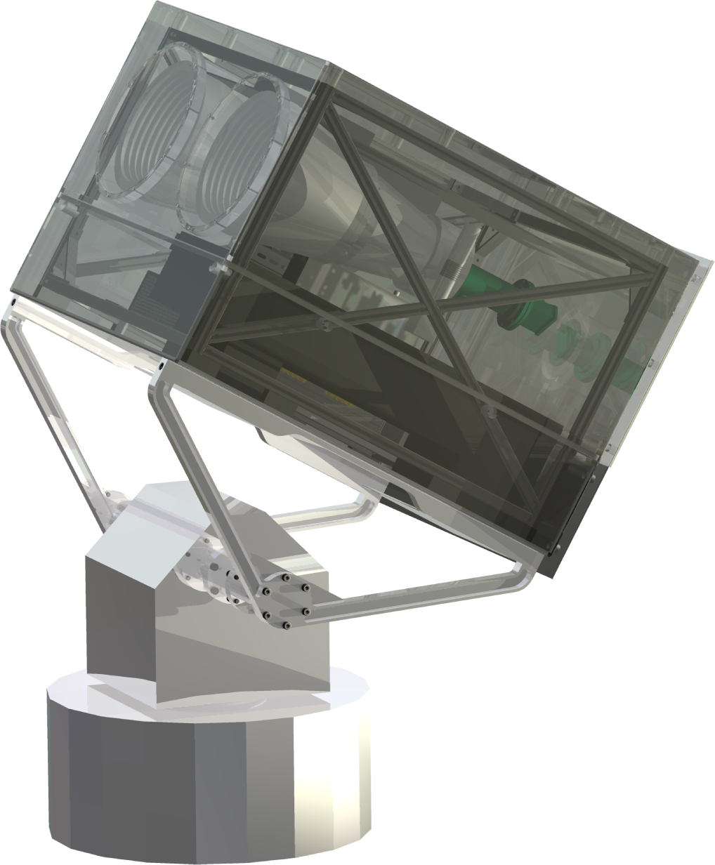
3.3. Reference Point Targets
3.4. Target Alignment
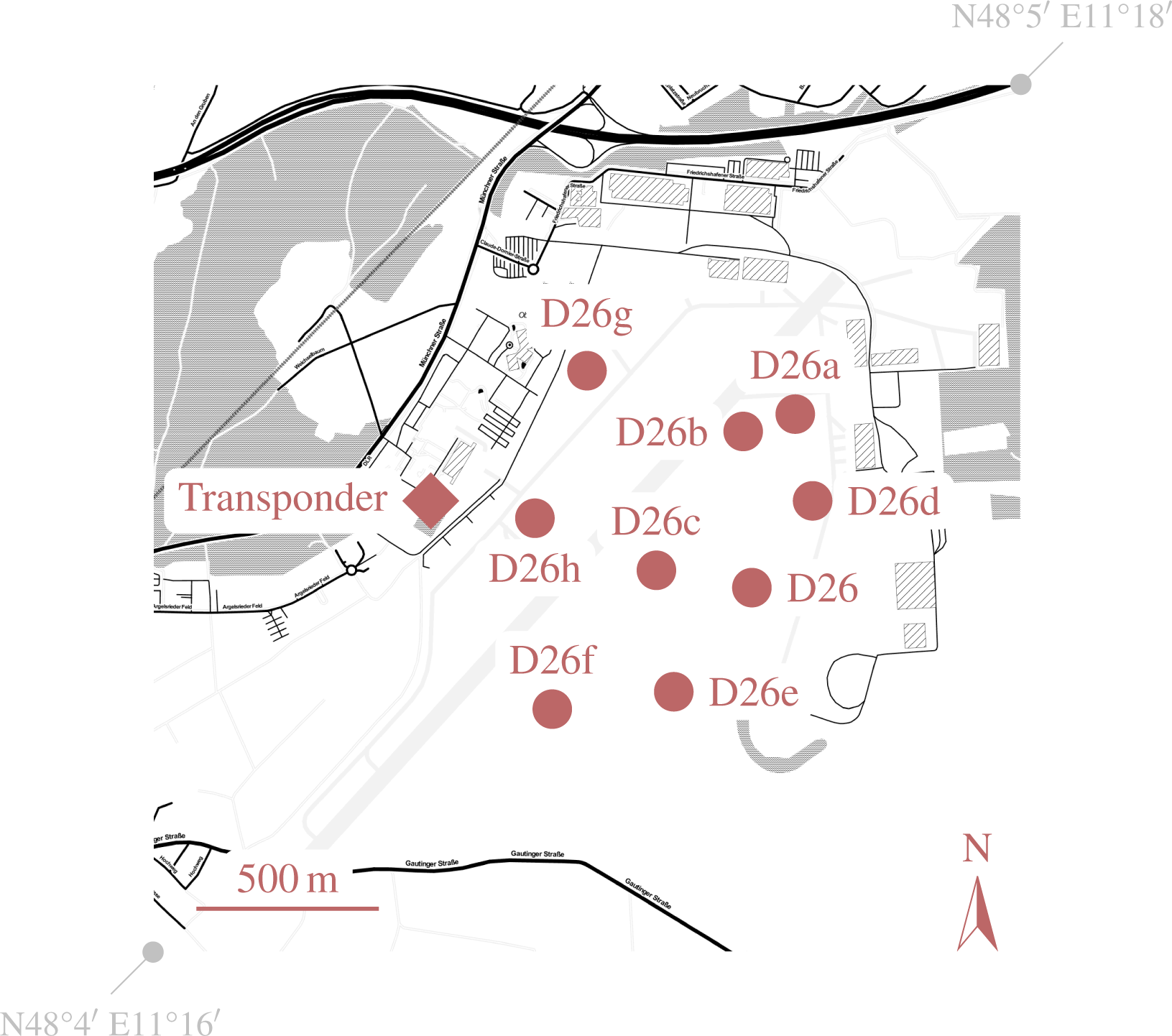
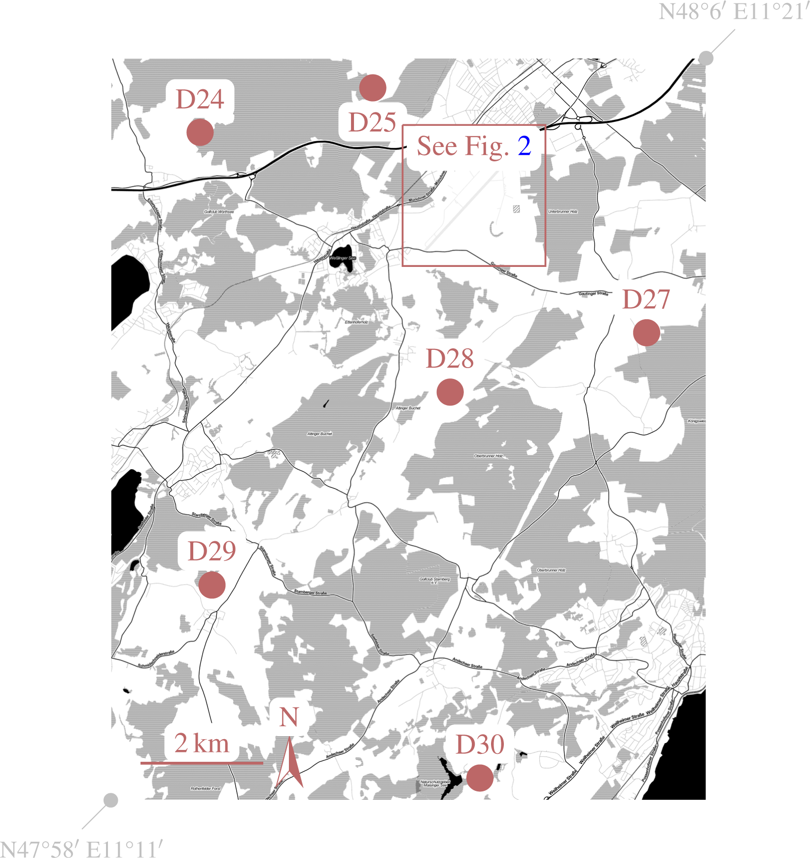
3.5. Imaged Area
4. Case Study: Data Analysis and Results
4.1. Overview
- Point target analysis: Extract the relative point target impulse response powers for all point targets in all scenes (see Section 4.2).
- Parameter estimation: Set up a statistical model to derive the estimated transponder ERCS and corresponding uncertainty from all datatakes (see Section 4.3).
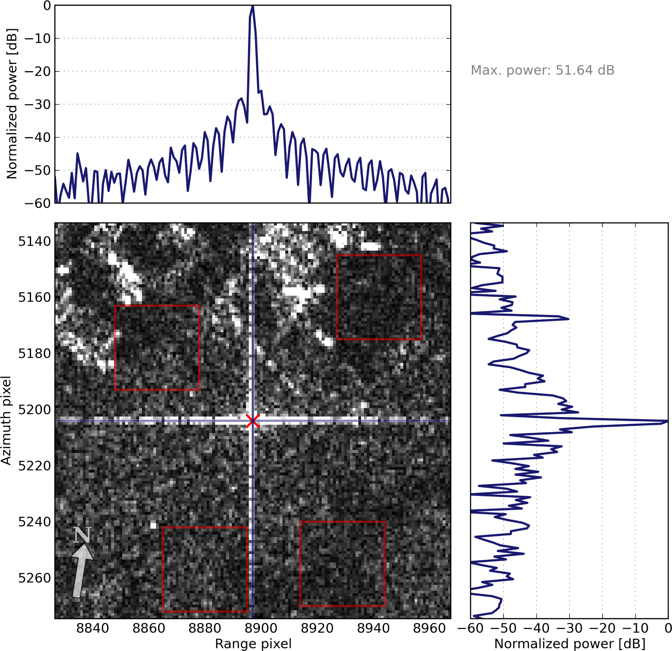
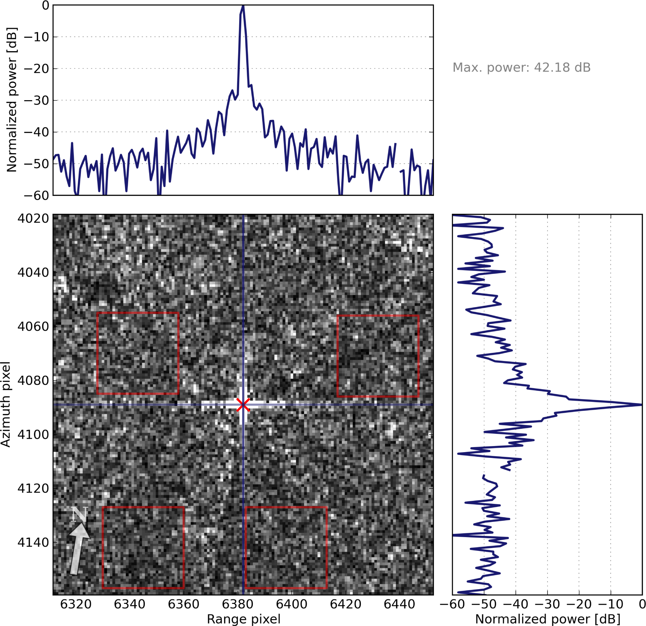
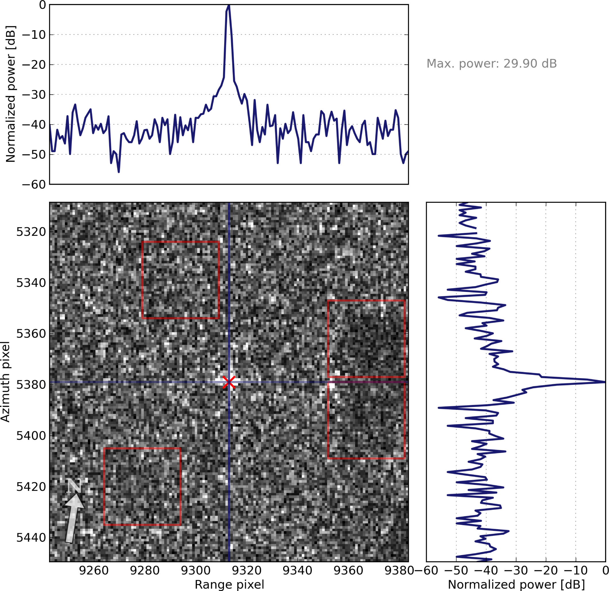
4.2. Power Estimation for Point Targets from SAR Images
- Define a search window around the point target in the georeferenced, processed image.
- Find and record the brightest pixel location.
- Define an analysis window, centered on the brightest pixel of the previous step.
- Estimate the clutter power from four non-overlapping areas surrounding the peak.
- Subtract the estimated clutter power from the integrated target power to get a clutter-compensated target power.
4.3. Bayesian Statistics and Hierarchical Model Fitting
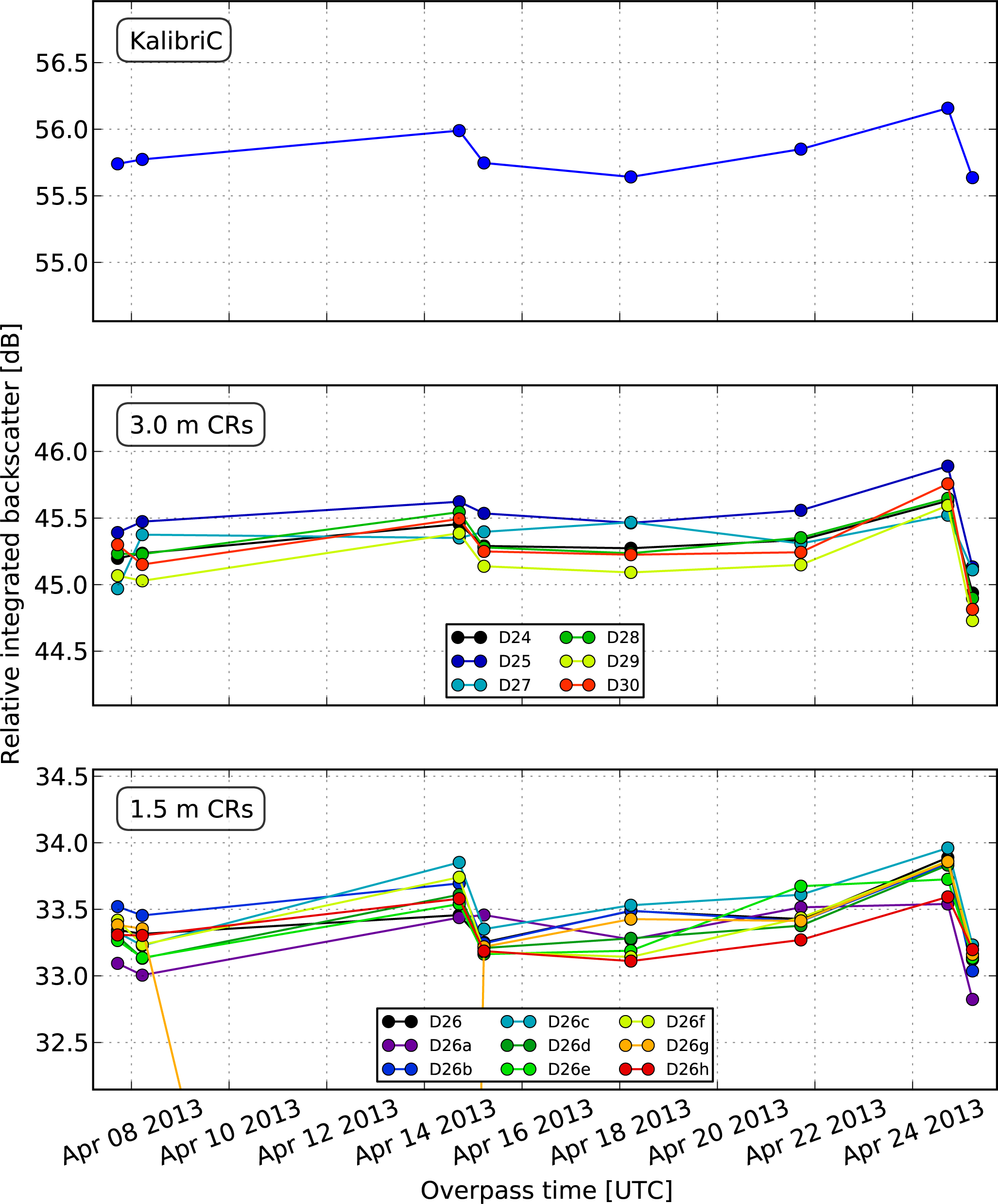
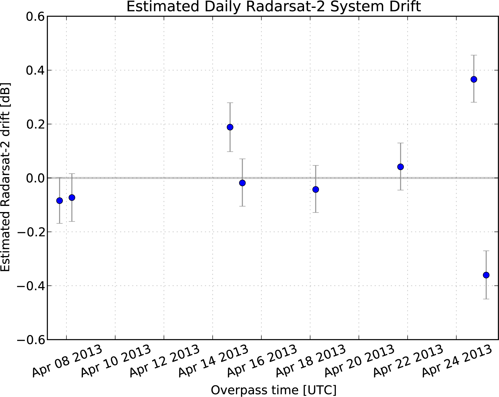
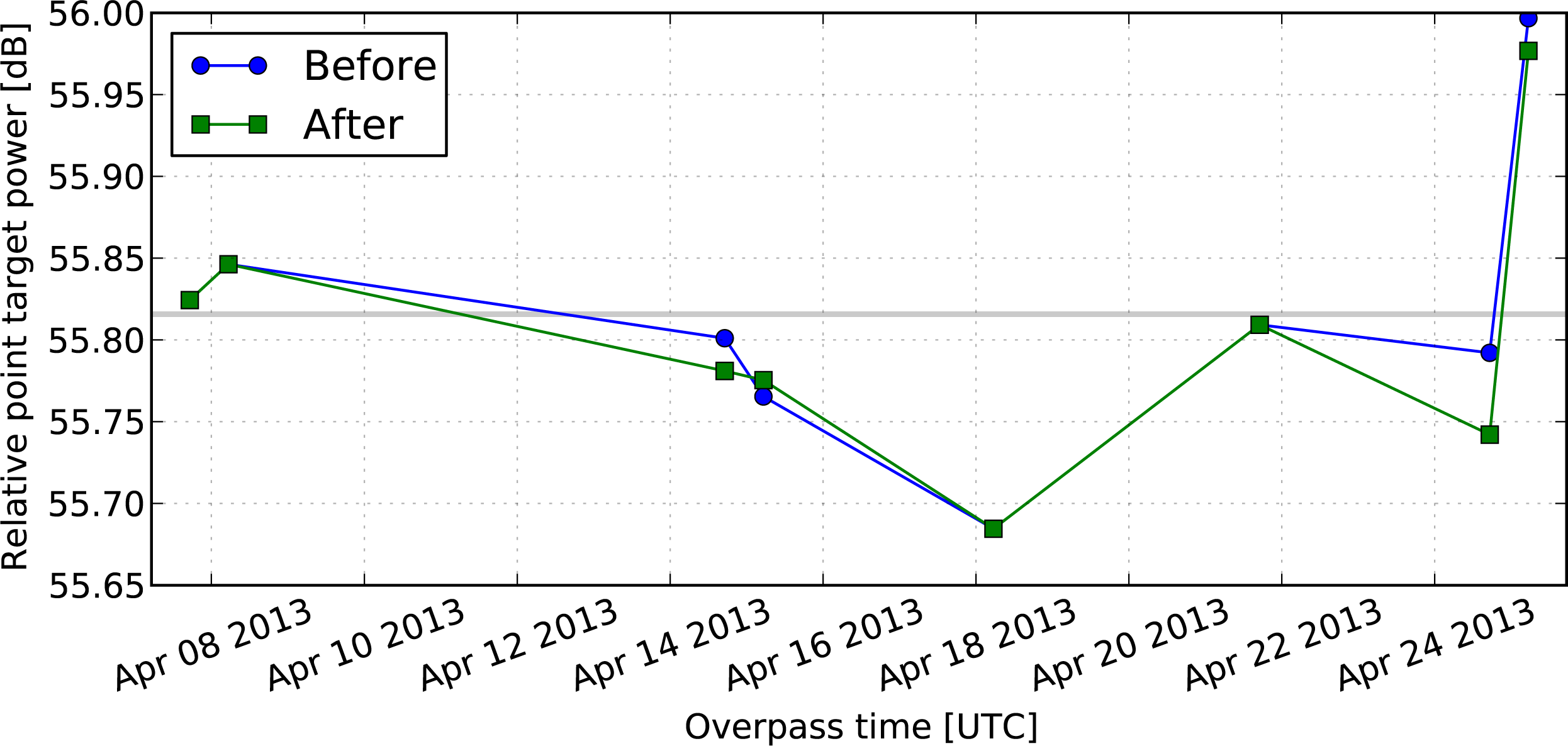
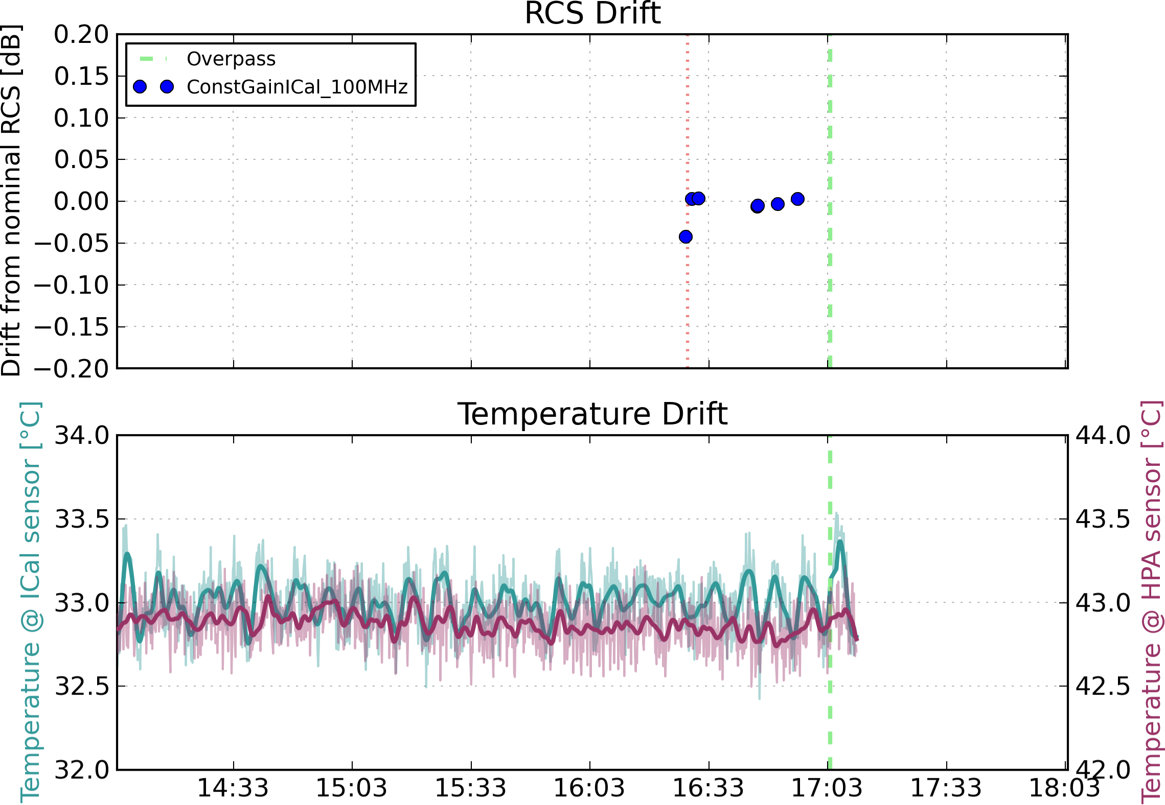
4.3.1. Daily RADARSAT-2 and Transponder Drifts
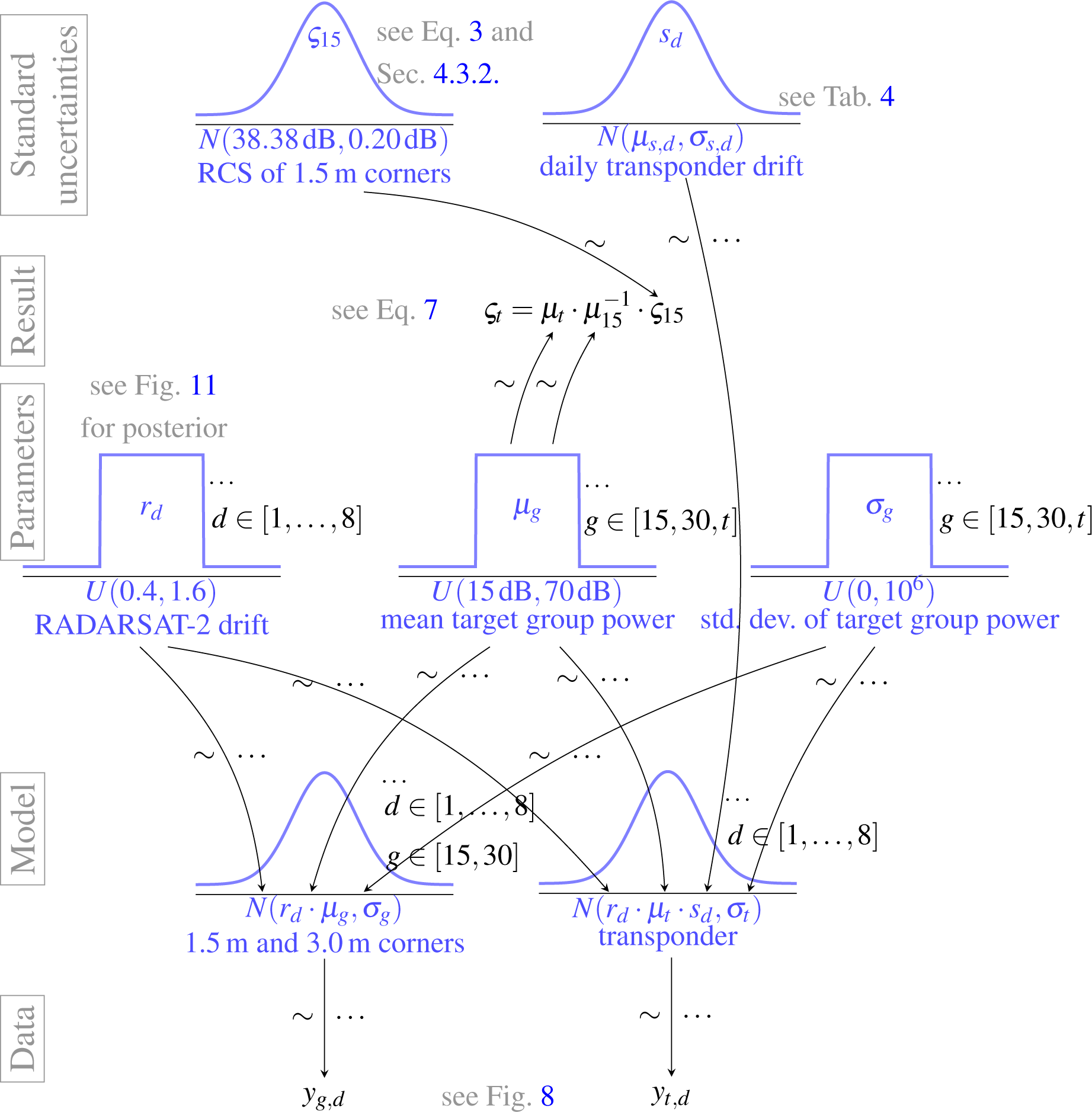
4.3.2. Hierarchical Bayesian Model
4.3.3. Posterior Simulation
4.3.4. MCMC Results
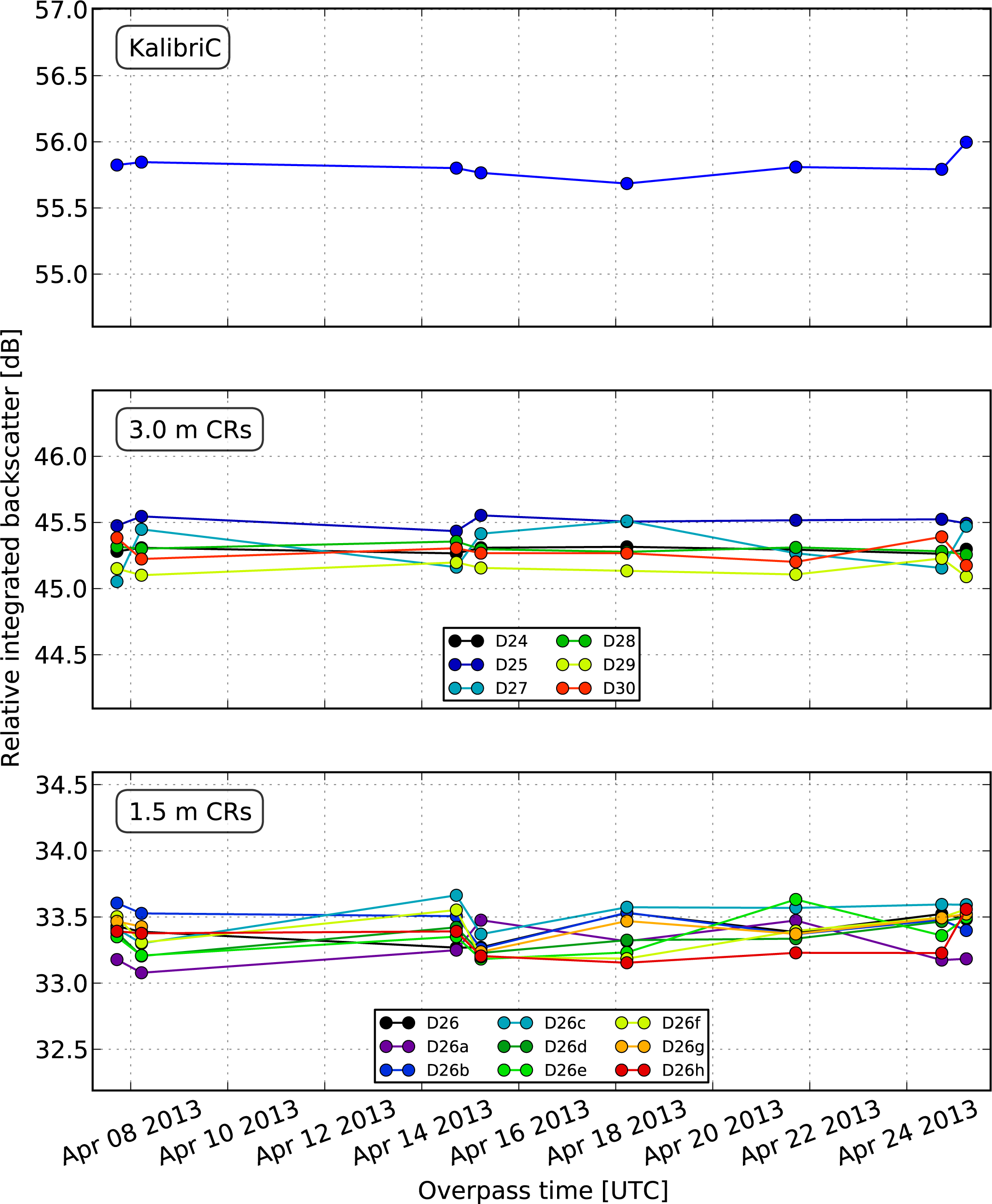
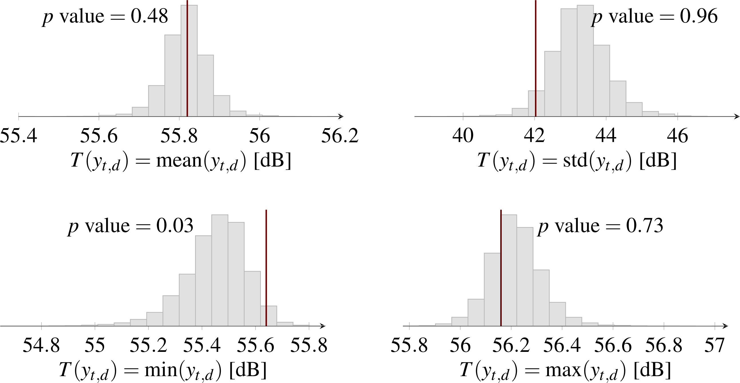
4.4. Posterior Predictive Checks: Model Verification
4.5. Plausibility Check with Classical Statistics
5. Discussion of Hierarchical Bayesian Data Analysis for Radiometric Calibration
6. Conclusions
- Within Bayesian statistics, probability distributions are used in describing model parameters. The distributions convey a meaning of uncertainty. Bayesian statistics is therefore an appropriate choice for calibration, where an estimated parameter is meaningless without a statement of its uncertainty.
- Hierarchical joint probability models are well suited to describe data that is typically acquired during an external radiometric SAR calibration campaign. During data analysis, depending on the research question, parameters often need to be estimated on different levels or for different groups. Hierarchical Bayesian modeling is well suited to derive model parameters for different interdependent parameters, especially when numerical methods like Markov chain Monte Carlo simulations are used.
Acknowledgments
Conflicts of Interest
References
- Van Zyl, J.J.; Kim, Y. Synthetic Aperture Radar Polarimetry; John Wiley & Sons, Inc: Hoboken, NJ, USA, 2011. [Google Scholar]
- Dobson, M.C.; Ulaby, F.T.; Letoan, T.; Beaudoin, A.; Kasischke, E.S.; Christensen, N. Dependence of radar backscatter on coniferous forest biomass. IEEE Trans. Geosci. Remote Sens. Electr 1992, 30, 412–415. [Google Scholar]
- Freeman, A. SAR calibration: An overview. IEEE Trans. GeoscI. Remote Sens 1992, 30, 1107–1121. [Google Scholar]
- Curlander, J.C. Synthetic Aperture Radar: Systems and Signal Processing; John Wiley & Sons, Inc: Hoboken, NJ, USA, 1991. [Google Scholar]
- Schwerdt, M.; Bräutigam, B.; Bachmann, M.; Döring, B.; Schrank, D.; Hueso Gonzalez, J. Final TerraSAR-X calibration results based on novel efficient methods. IEEE Trans. Geosci. Remote Sens 2010, 48, 677–689. [Google Scholar]
- Shimada, M.; Isoguchi, O.; Tadono, T.; Isono, K. PALSAR radiometric and geometric calibration. IEEE Trans. Geosci. Remote Sens 2009, 47, 3915–3932. [Google Scholar]
- Evaluation of Measurement Data—Guide to the Expression of Uncertainty in Measurement; ISO/IEC Guide 98-3:2008; ISO copyright office: Geneva, Switzerland, 2008.
- Schwerdt, M.; Hueso Gonzalez, J.; Bachmann, M.; Schrank, D.; Döring, B.; Tous Ramon, N.; Walter Antony, J.M. In-Orbit Calibration of the TanDEM-X System. Proceedings of the IEEE International Geoscience and Remote Sensing Symposium, Vancouver, BC, Canada, 24–29 July 2011; pp. 2420–2423.
- Luscombe, A.P.; Thompson, A.A. RADARSAT-2 Calibration: Proposed Targets and Techniques. Proceedings of the IEEE International Geoscience and Remote Sensing Symposium, Vancouver, BC, Canada, 24–29 July 2001; pp. 496–498.
- Luscombe, A. Image Quality and Calibration of RADARSAT-2. Proceedings of the IEEE International Geoscience and Remote Sensing Symposium, Cape Town, South Africa, 12–17 July 2009; pp. 757–760.
- Chakraborty, M.; Panigrahy, S.; Rajawat, A.S.; Kumar, R.; Murthy, T.V.R.; Haldar, D.; Chakraborty, A.; Kumar, T.; Rode, S.; Kumar, H.; et al. Initial results using RISAT-1 C-band SAR data. Curr. Sci 2013, 104, 490. [Google Scholar]
- Gelman, A.; Carlin, J.B.; Stern, H.S.; Rubin, D.B. Bayesian Data Analysis, 2nd ed; Chapman & Hall/CRC: Boca Raton, FL, USA, 2004. [Google Scholar]
- Gregory, P. Bayesian Logical Data Analysis for the Physical Sciences; Cambridge University Press: Cambridge, UK, 2005. [Google Scholar]
- Bayarri, M.J.; Berger, J.O. The interplay of bayesian and frequentist analysis. Stat. Sci 2004, 19, 58–80. [Google Scholar]
- Döring, B.J.; Schwerdt, M. The radiometric measurement quantity for SAR images. IEEE Trans. Geosci. Remote Sens. 2013. [Google Scholar] [CrossRef] [Green Version]
- Bolstad, W.M. Introduction to Bayesian Statistics, 2nd ed; John Wiley & Sons, Inc: Hoboken, NJ, USA, 2007; p. 464. [Google Scholar]
- Patil, A.; Huard, D.; Fonnesbeck, C.J. PyMC: Bayesian stochastic modelling in Python. J. Stat. Softw 2010, 35, 1–81. [Google Scholar]
- Döring, B.J.; Looser, P.; Jirousek, M.; Schwerdt, M.; Peichl, M. Highly Accurate Calibration Target for Multiple Mode SAR Systems. Proceedings of the European Conference on Synthetic Aperture Radar, Aachen, Germany, 7–10 June 2010; 8.
- MDA Corporation. Radarsat-2 Product Description; MacDonald, Dettwiler and Associates Ltd: Richmond, BC, Canada, 2011. [Google Scholar]
- Oerry, A.W.; Brock, B.C. Radar Cross Section of Triangular Trihedral Reflector with Extended Bottom Plate; Technical Report May; Sandia National Laboratories: Albuquerque, NM, USA, 2009. [Google Scholar]
- Gray, A.L.; Vachon, P.W.; Livingstone, C.E.; Lukowski, T.I. Synthetic aperture radar calibration using reference reflectors. IEEE Trans. Geosci. Remote Sens 1990, 28, 374–383. [Google Scholar]
- Dettwiler, M. RADARSAT-2 Product Format Definition; Technical Report 1/9; MacDonald, Dettwiler and Associates Ltd: Richmond, Canada, 2011. [Google Scholar]
- Schwerdt, M.; Döring, B.; Zink, M.; Schrank, D. In-Orbit Calibration Plan of Sentinel-l. Proceedings of the European Conference on Synthetic Aperture Radar, Aachen, Germany, 7–10 June 2010; pp. 350–353.
- Weise, K.; Wöger, W. A Bayesian theory of measurement uncertainty. Meas. Sci. Technol. 1992. [Google Scholar] [CrossRef]
- Kacker, R.; Jones, A. On use of Bayesian statistics to make the Guide to the Expression of Uncertainty in Measurement consistent. Metrologia 2003. [Google Scholar] [CrossRef]
- Willink, R.; White, R. Disentangling Classical and Bayesian Approaches to Uncertainty Analysis; Technical Report No. CCT/12-08; BIPM: Sevres, France, 2012. [Google Scholar]


| Overpass Time | Orbit Direction | Beam Mode |
|---|---|---|
| 7 April 2013 17:11:09 | ascending | U17W2 |
| 8 April 2013 05:20:16 | descending | U16W2 |
| 14 April 2013 17:06:59 | ascending | U11W2 |
| 15 April 2013 05:16:06 | descending | U22W2 |
| 18 April 2013 05:28:36 | descending | U5W2 |
| 21 April 2013 17:02:49 | ascending | U5W2 |
| 24 April 2013 17:15:19 | ascending | U22W2 |
| 25 April 2013 05:24:26 | descending | U10W2 |
| Size | Peak RCS | Number of Targets |
|---|---|---|
| 1.5 m | 38.38 dBm2 | 9 |
| 3.0 m | 50.43 dBm2 | 6 |
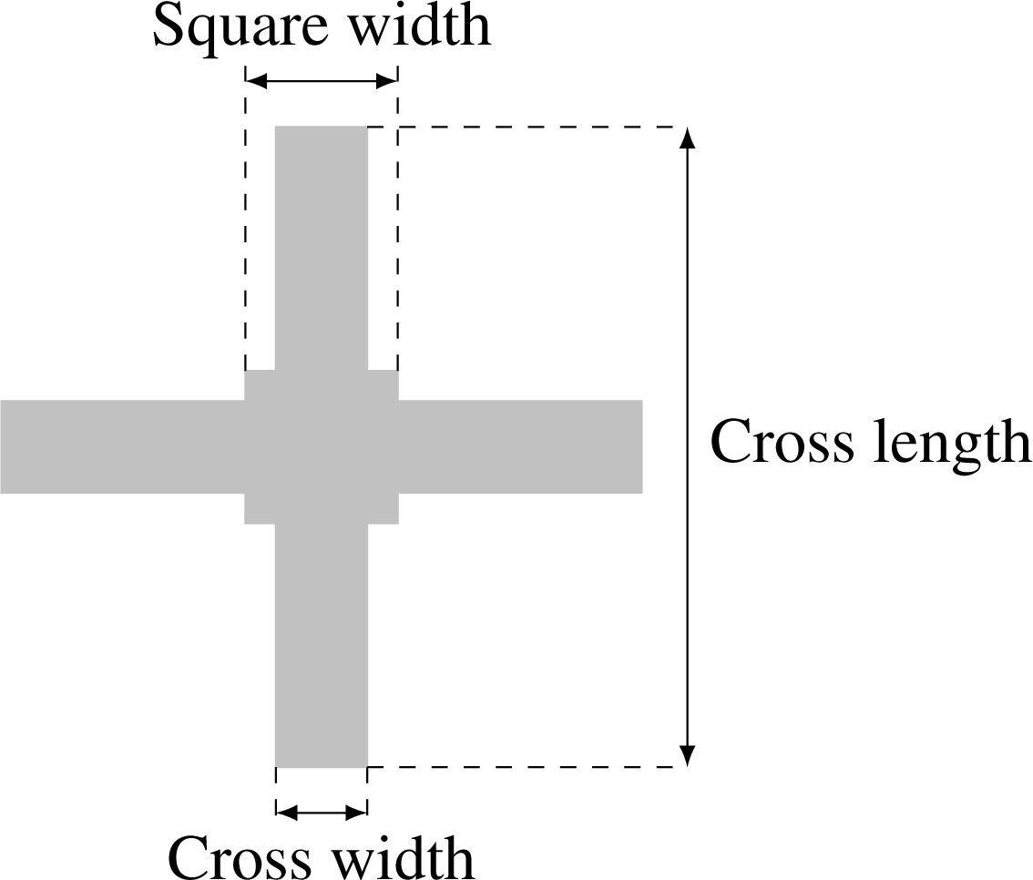
| Parameter | Pixels |
|---|---|
| Cross length | 21 |
| Cross width | 3 |
| Square width | 5 |
| Overpass Date | Estimated Drift μs (dB) | Maximal Error (dB) | Resulting σs (dB) |
|---|---|---|---|
| 2013-04-07 | 0.00 | 0.05 | 0.03 |
| 2013-04-08 | 0.00 | 0.02 | 0.01 |
| 2013-04-14 | 0.02 | 0.03 | 0.02 |
| 2013-04-15 | −0.01 | 0.03 | 0.02 |
| 2013-04-18 | 0.00 | 0.07 | 0.04 |
| 2013-04-21 | 0.00 | 0.02 | 0.01 |
| 2013-04-24 | 0.05 | 0.05 | 0.03 |
| 2013-04-25 | 0.02 | 0.03 | 0.02 |
© 2013 by the authors; licensee MDPI, Basel, Switzerland This article is an open access article distributed under the terms and conditions of the Creative Commons Attribution license ( http://creativecommons.org/licenses/by/3.0/).
Share and Cite
Döring, B.J.; Schmidt, K.; Jirousek, M.; Rudolf, D.; Reimann, J.; Raab, S.; Antony, J.W.; Schwerdt, M. Hierarchical Bayesian Data Analysis in Radiometric SAR System Calibration: A Case Study on Transponder Calibration with RADARSAT-2 Data. Remote Sens. 2013, 5, 6667-6690. https://doi.org/10.3390/rs5126667
Döring BJ, Schmidt K, Jirousek M, Rudolf D, Reimann J, Raab S, Antony JW, Schwerdt M. Hierarchical Bayesian Data Analysis in Radiometric SAR System Calibration: A Case Study on Transponder Calibration with RADARSAT-2 Data. Remote Sensing. 2013; 5(12):6667-6690. https://doi.org/10.3390/rs5126667
Chicago/Turabian StyleDöring, Björn J., Kersten Schmidt, Matthias Jirousek, Daniel Rudolf, Jens Reimann, Sebastian Raab, John Walter Antony, and Marco Schwerdt. 2013. "Hierarchical Bayesian Data Analysis in Radiometric SAR System Calibration: A Case Study on Transponder Calibration with RADARSAT-2 Data" Remote Sensing 5, no. 12: 6667-6690. https://doi.org/10.3390/rs5126667