1. Introduction
Ocean surface winds from scatterometers and synthetic aperture radars (SAR) are useful for oceanic and atmospheric modeling, hurricane tracking, air-sea interaction studies, oil spill monitoring and marine safety, amongst others. Such observations are also becoming more applicable for wind resource assessment offshore, where in situ measurements are difficult to obtain. While both sensors were operational for nearly a decade, the QuikSCAT (Quick Scatterometer) products combined daily coverage of approximately 90% of the global ocean with a spatial resolution of 25 km. ENVISAT (Environmental Satellite) Advanced SAR (ASAR) ocean wind retrievals have a much higher spatial resolution, up to 600 m, but an inconsistent spatial and infrequent temporal coverage of a given area, Thus, satellite wind maps provide a wide range of spatial resolutions for examining the offshore wind characteristics.
Both QuikSCAT and SAR products are currently used for offshore wind resource assessment. Studies have used a gridded QuikSCAT product from remote sensing systems (RSS) to evaluate wind characteristics in the North Sea [
1,
2]. Winds retrieved from ENVISAT ASAR are also used for wind resource assessment [
3–
5]. Direct comparisons between QuikSCAT and ENVISAT ASAR wind products are limited by differences in the spatial resolution and the approximately five-hour time lag between overpass times in the North Sea. The purpose of this study is to examine the spectral properties of the near-surface winds retrieved from the two sensors, and in this case, the spatial and temporal mismatches are not crucial.
The spectral properties of surface winds are fundamental for oceanic modeling and are used as a measure of accuracy for short-term forecasting in the meso-scale range [
6] and for estimating extreme winds [
7]. The spectral properties are also essential in order to understand the nature of spatially coherent surface winds in terms of the effective spatial resolution of different products. Moreover, for offshore conditions, satellite datasets provide a wide spatial coverage of the wind distribution, thus complementing our understanding of the wind variability at larger scales, which, currently, is significantly based on limited point
in situ measurements.
Early investigations of wind spectra have shown a dependency of the spectral energy on the wavenumber, k. For wavelengths smaller than approximately 400 km, in log-log scale, the wind velocity spectra, S(k), decrease with the wavenumber along a −5/3 slope, while for wavelengths in the range of 1,000–3,000 km, the decrease has a slope closer to −3 [
8]. While the −3 slope was interpreted through the geostrophic turbulence theory as a result of the transfer of entropy from the larger to smaller scales, the interpretation of the −5/3 slope has not reached a consensus.
The spectral properties of the Seasat-A scatterometer (SASS) near-surface winds showed a dependency of the computed spectra on k
−2 for the mid-latitudes and for length scales from 200 to 2,200 km [
9]. Spectral comparison of wind products from QuikSCAT and the Advanced Scatterometer (ASCAT), on the MetOp (Meteorological Operational) -A and -B platforms, showed that the ASCAT-25 km product contains more intermediate scale information than the QuikSCAT product processed at the Royal Netherlands Meteorological Institute (KNMI) [
10]. Spectral analysis of different QuikSCAT products in the Pacific Ocean showed that for wavenumbers in the meso-scale and for length scales from 50 to 1,700 km, the slope ranged from −2.2 to −2.4 [
11].
Scatterometer winds from the European Remote Sensing Satellite 1 (ERS-1) for the range of 50–1,800 km had slopes of −2.6 and −2.4 along the zonal and meridional wind directions, respectively [
12]. Scatterometer winds from ERS-1, re-analysis winds from NCEP (National Centers for Environmental Prediction) and high resolution aircraft observations for a wavenumber range corresponding to scales from one to 1,000 km showed the best fit slope from the combined spectra very near the −5/3 law and a lack of realistic variability in the modeled winds at length scales smaller than 1,000 km [
13].
In the process of refining the framework for wind retrieval from SAR images, it was found that the computed spectra from SAR winds retrieved at different resolutions had lower spectral density levels as the resolution decreased and shared similarities with spectra computed from measurements taken during a flight [
14]. For a single ERS-1 SAR wind map retrieved with a 200 m grid cell resolution, produced after averaging of the 25 m × 25 m cells, a slope around −1.1 was reported for length scales between 100 and 2 km [
15].
The studies above demonstrate the established usability of satellite wind products for the examination of the spectral characteristics of surface winds and the effective resolution of different space-borne sensors. While QuikSCAT winds have been extensively used for spectral comparisons, the literature regarding SAR spectra is limited. Moreover, the impact of varying resolution amongst satellite winds is an ongoing research topic [
10].
In this paper, we aim to examine the spectral properties of ENVISAT ASAR (to be used interchangeably with SAR) winds retrieved at varying resolutions and compare them with the QuikSCAT-derived spectra. It is also of interest to evaluate the quality of the preserved length scales amongst the SAR products and to examine their effective spatial resolution. In particular, the very high resolution 600-m SAR product may provide spectral information not observable from other sensors. This is presented in Section 4.1 by means of estimating the resolvable length scales in the spatially averaged wind products and examining their power law behavior.
As the SAR wind retrievals over a given area are not temporally coherent, the impact of the available sample size in the derived spectra is examined and presented in Section 4.2. Seasonal spectra are also computed and presented in Section 4.3, to identify any potential seasonal variability. A discussion on the findings is presented in Section 5, and the key findings are summarized in Section 6.
3. Methods
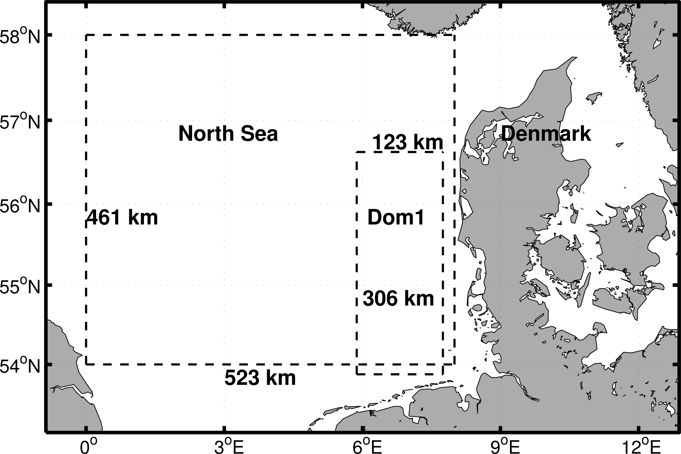
Two study areas are used, shown in
Figure 1. The entire North Sea (NS) has an area of approximately 75 × 10
4 km
2 and an average water depth of 90 m. It is located within the Northern Hemisphere, where strong prevailing westerly winds are frequent. A sub-domain (Dom1) is selected, due to the overlap of SAR images; 135 scenes were retrieved from the archive and 100 were coincident with QuikSCAT.
Due to the lag in the local equatorial crossing time of QuikSCAT (∼06:00, 18:00) and the ENVISAT platform (∼10:00, 22:00), time-collocation is performed by selecting the same date and fraction of day. Rain contaminated QuikSCAT data are flagged, and a maximum data loss of 20% is allowed for each QuikSCAT pass. If the number of rain-contaminated grid cells, in a single wind map, exceeds 20% of the total number of grid cells in this given QuikSCAT wind scene, both the QuikSCAT and the corresponding SAR retrieval are discarded. This reduced the total number of available scenes to 87. The average characteristics of the satellite passes are shown in
Table 1, while in brackets are the amounts of rain-free QuikSCAT scenes available from the 10 year-long archive.
Spatial series of the horizontal wind speed are extracted along the west-east (zonal) and north-south (meridional) directions, but no decomposition of the horizontal wind vector is performed. Each spatial series is linearly detrended prior to the Fast Fourier Transform (FFT). The spectra from all the transects along the zonal and meridional directions are afterwards time-averaged. Spectral slopes are estimated for each dataset by fitting a line to the spectrum, but excluding the highest wavenumber part, i.e., wavenumbers from 10−5 and up to 5 × 10⁻³ rad·m−1 are included. The standard deviation (σ) of the average power spectra, S(k), is also computed from all the transects of the time-average spectra along the zonal and meridional direction, correspondingly. It is shown as a shaded area around the averaged spectra, bounded by the curves S(k) ± 1σ in a log-log scale.
For QuikSCAT and in sub-domain Dom1, the number of spectral nodes,
i.e., grid cells in the spatial time-series available for the FFT, is 12 along the meridional and eight along the zonal direction. In order to establish the reliability of the QuikSCAT-derived spectra in such a small domain, spectra are also computed for a squared domain that includes most of the North Sea (54°–58°N, 0°–8°E; see
Figure 1). SAR wind maps are treated exactly as the QuikSCAT ones, but only Dom1 is covered.
The impact of the effective spatial resolution of the QuikSCAT and SAR winds is examined in Section 4.1 by means of the spectral density in the resolved wavenumber range and the spectral slopes. The sample size used for the spectral computations consists of 87 scenes for the different datasets. The size of the sub-domain, Dom1, results in a rather limited number of spectral nodes for the coarser resolution products. In addition, QuikSCAT spectra computed from the same set of 87 scenes, but for the larger North Sea domain, are also presented (QSCAT NS). This is expected to provide an insight into the impact of limited spectral nodes. In all the legend entries, QuikSCAT is abbreviated to QSCAT.
Regarding the limited number of available SAR near-surface wind scenes, the impact of the sample size on the spectral behaviors is investigated in Section 4.2 using the QuikSCAT dataset consisting of 87 scenes and the full QuikSCAT dataset (labeled as QSCAT-10y) with 5,626 scenes. In addition, the impact of the domain size in relation to the sample size is addressed by examining the QuikSCAT spectra computed for the sub-domain, Dom1 (QSCAT Dom1), and those computed for the larger North Sea domain (QSCAT NS).
Finally, spectra from the spatial series are averaged in seasons and are presented in Section 4.3. The impact of the sample size on the seasonal spectra is examined with comparisons of the QuikSCAT 87 scenes against the full dataset, while the seasonal spectra’s sensitivity to the domain size is investigated through the spectra from the smaller Dom1 and larger North Sea domains.
4. Results
4.1. On the Spatial Resolution
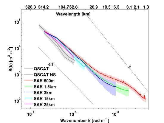
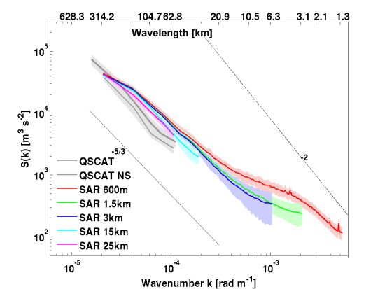
Figure 2 shows the average power spectra as a function of wavenumber (bottom axis) and length scale (top axis) in a log-log scale, along the (a) meridional and (b) zonal directions of the QuikSCAT (gray, solid lines) and SAR (in color) winds. There is a rather good agreement between the spectra of the SAR data of various resolutions for wavelengths greater than about 60 km. SAR wind spectra show higher spectral density than the QuikSCAT spectra in general, but the two converge at larger scales. A general dependence of the spectral density on the resolution is identified through: (i) the SAR data for wavelengths smaller than about 30 km; (ii) the SAR data with wavelengths greater than 30 km when the resolution is 15 km or coarser (blue and magenta curves); and (iii) the QuikSCAT data (gray curves) compared to the SAR data for wavelengths greater than about 60 km. The SAR-600 m product shows the highest energy content for length scales down to 3 km. In particular, for length scales smaller than 30 km, an increasing difference in the spectral density is identified between the SAR 600-m (red) and the SAR 1.5-km (green) products.
At the same resolution, the 25-km SAR product (magenta) shows higher spectral content than the corresponding QuikSCAT product (thin gray line), along the meridional and zonal directions. This can be partly attributed to a reduced variance of the QuikSCAT product, due to the smoothing effect caused by the interpolation schemes used to produce the gridded L3 data [
19]. This smoothing effect may eliminate smaller scale variability, which will be manifested as a reduced spectral density level and could potentially be avoided by using swath rather than gridded winds.
QuikSCAT spectral tails turn and become flat for length scales around 60 km, clearly observed along the zonal direction. Stoffelen
et al. [
20] attributed a similar behavior of the QuikSCAT-NOAA product to the noise in the nadir part of the swath occurring, due to the measuring geometry, which affects the wind direction retrieval. The SAR 1.5 and 3-km products also show a tendency of flattening spectra for scales close to 6 km.
The number of available spectral nodes in the 25-km products is low for the sub-domain, Dom1. The spatial coverage of QuikSCAT consistently extends to the entire North Sea, which gives higher reliability for the spectrum calculation for large scales. Accordingly, the spectra along the meridional and zonal direction were calculated for the entire NS domain, based on the same set of 87 wind scenes. These spectral components are shown in
Figure 2, labeled as QSCAT NS, and have a larger wavenumber range, which extends towards lower values (larger length scales), due to the larger domain dimensions. By examining the QuikSCAT spectra (gray solid lines) for Dom1 (thin) and NS (thick) in
Figure 2, it is found that the spectral density levels increase when the domain size increases, which is likely related to the inclusion of the more energetic, synoptic atmospheric movements.
Along the meridional direction, QuikSCAT spectra show relatively constant standard deviation as the wavenumber increases. That of the SAR spectra tends to be smaller for the smaller wavenumbers and increases as the wavenumber becomes larger. This is most obvious for the 1.5, 3 and 15-km products, while it does not happen for the 25-km one. The 600-m SAR product also shows a relatively constant σ, which is nonetheless larger than the 25-km one. Along the zonal direction, spectra have generally larger σ values, strengthening the assumption that the small domain size in this direction introduces uncertainties in the computed spectra. Especially for the 1.5, 3 and 15-km SAR products, the lower curve, S(k)–1σ, becomes negative for wavelengths smaller than 25 km, and thus, the last positive value is used to create the shaded areas around the curves. Nonetheless, the 600-m SAR product has the smallest σ, which does not vary as the wavenumber, k, increases.
Spectral slopes are estimated for each product by excluding the highest wavenumber part of the corresponding spectrum and, thus, are valid for the meso-scale range from ∼600 km down to the meso/micro-scale range at ∼2 km. Slopes range from −0.99 to −1.8, with the along meridional QuikSCAT slopes closest to −5/3 (
Table 2). SAR slopes are flatter for very high resolutions and become larger as the resolution decreases. The 25-km SAR meridional slope is flatter than QuikSCAT, but the opposite occurs along the zonal direction. Flatter slopes indicate a smaller energy deficit for increasing wavenumbers; thus, smaller length scales may be resolvable by the satellite product. This finding demonstrates the higher effective spatial resolution achievable by the SAR retrieved winds compared to the QuikSCAT 25-km product.
For the very end of the high wavenumber range,
i.e. the smallest resolvable wavelengths, the uncertainty introduced by the potential speckle noise contamination, and the potential signature of surface currents and internal waves could be considerable, causing the smaller slope in the 600-m product when compared to the rest of the products and for wavelengths smaller than 30 km. Nonetheless, the significantly higher spectral density in the 600-m product possibly suggests an energy feeding from small scales, a theory long argued [
8]. This energy feeding from small scales to larger scales is less resolved in the 1.5-km data. We might expect an even different picture of the slope when even finer data are used.
The overall smallest deviation from the −5/3 law is found for the QuikSCAT along the meridional direction computed for the North Sea domain. Slopes along the zonal direction generally deviate from the −5/3 law the most, both for the SAR and QuikSCAT products. Minimal deviations from the −5/3 law along the zonal direction are computed for the North Sea QuikSCAT spectra. Thus, with the extension of the domain to account for spectra in the meso/macro-scale range (North Sea domain), an increase in the spectral content is observed along with a better fit of the spectral decay to the theory.
4.2. On the Sample Size
The sample size of the near-surface wind maps is limited by the availability of SAR scenes for the Dom1 study area. QuikSCAT has the advantage of consistent spatial and temporal coverage, with 10 years of twice daily observations. The representativeness of the sample size consisting of 87 wind maps is evaluated against the 10 year-long spectral estimates.
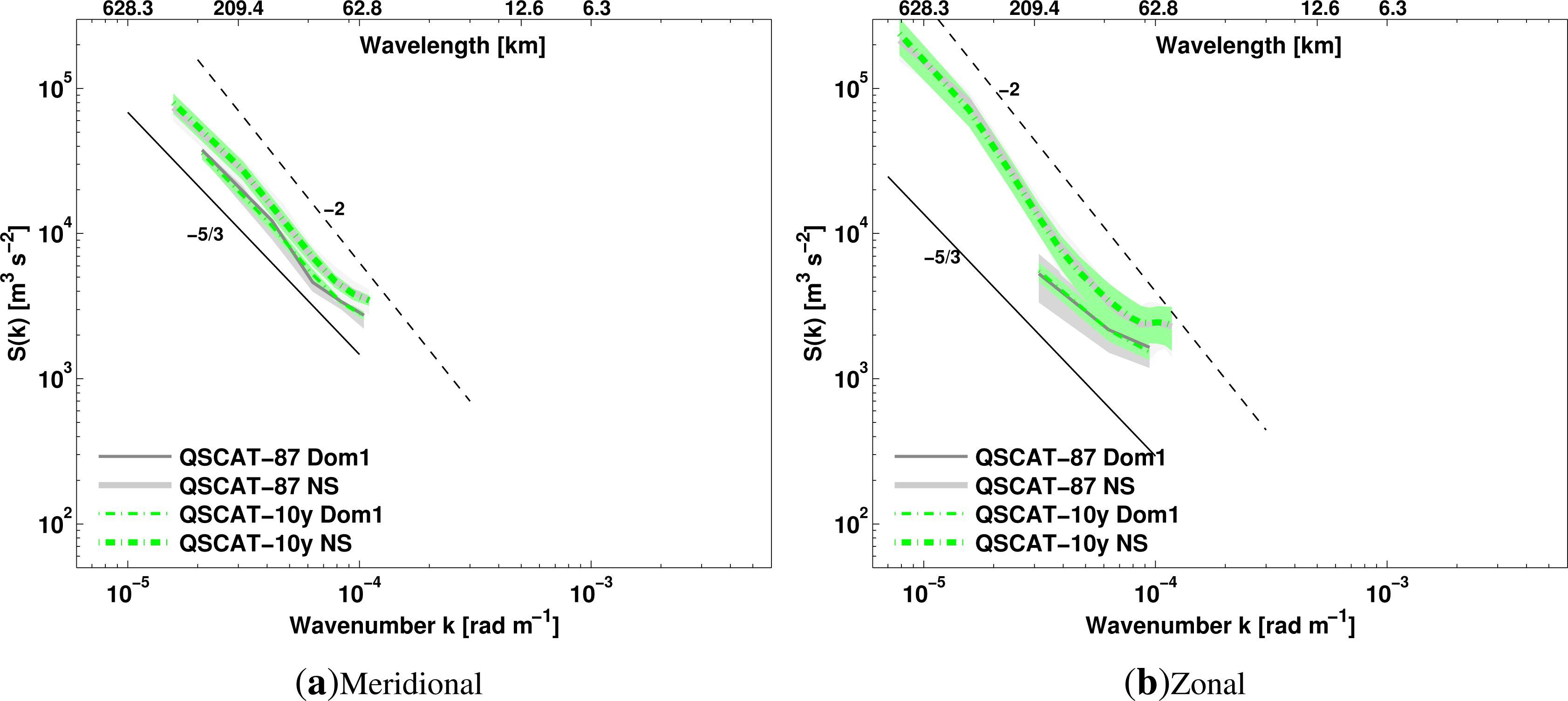
Figure 3 shows the averaged power spectra computed from 87 and 5,626 QuikSCAT wind maps, as a function of the wavenumber k (bottom axis), and wavelength (top axis) in a log-log scale and along the (a) meridional and (b) zonal directions.
No significant difference in the spectra is found between the two datasets, for both Dom1 (thin lines) and the NS domain (thick lines). The standard deviation σ, shown as a light gray or green area bounded by the curves S(k) ± 1σ, is smaller along the meridional than the zonal direction, independent of domain or sample size. Average spectra for the North Sea have the same σ values independent of sample size (thick gray line for the 87 scenes and thick, green dashed line for the 5,626-scene set). For the sub-domain Dom1, long-term spectra (thin green dashed lines) have smaller σ values compared to the 87-scene subset (thin gray lines), and this is more evident along the zonal direction. From such findings, it can be concluded that a total of 87 wind maps is representative of the longer term spectra derived from 5,626 wind scenes. For sizes greater than 87 scenes, the spectral properties appear to be independent of the sample size.
QuikSCAT spectral slopes shown in
Table 2 along the meridional direction range from −1.65 to −1.7 and along the zonal direction, from −1.1 to −1.8. The slope differences due to the sample size do not exceed 0.1 along both directions and are considered insignificant. The domain size has a more pronounced impact on the spectra. Higher spectral density levels are observed for the larger North Sea domain compared to the smaller Dom1, along both the meridional and zonal directions. Along the meridional direction, the difference in spectral density arising from the different domain size is rather constant for the entire wavenumber range. Along the zonal direction, for which
σ values are larger, this difference is larger for the lower wavenumber range (larger length scales) and becomes smaller as the wavenumber increases. This feature is likely associated with uncertainties arising from the small Dom1 size, as the short west–east range provides very few available spectral nodes.
The above hypothesis regarding the uncertainties of the spectra along the zonal direction due to the domain size is further supported by the slope differences. While along the meridional direction, the slope differences due to the domain size are in the order of 0.05, they are significantly larger along the zonal direction (∼0.7). Thus, zonal spectra in the sub-domain Dom1 are likely misrepresented by the coarser resolution wind products.
4.3. On the Seasonal Variability
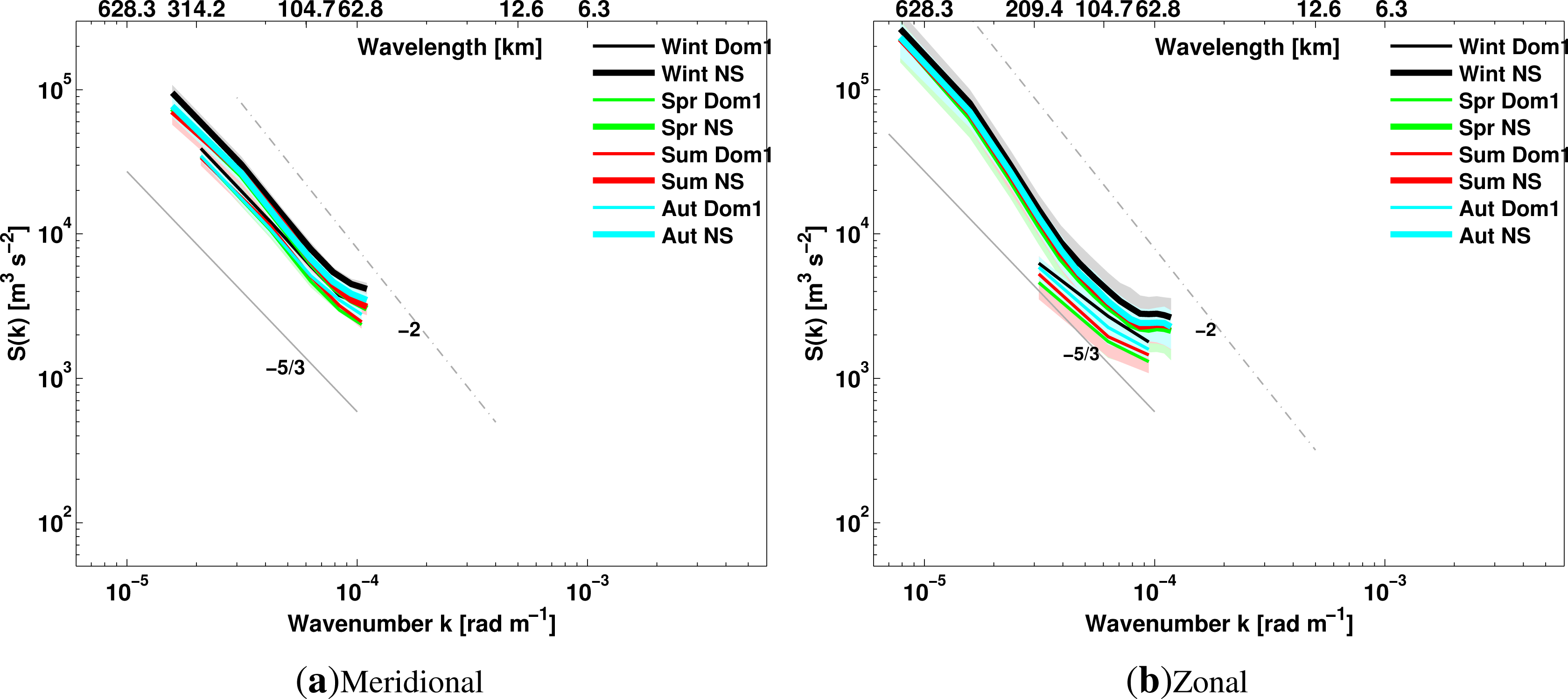
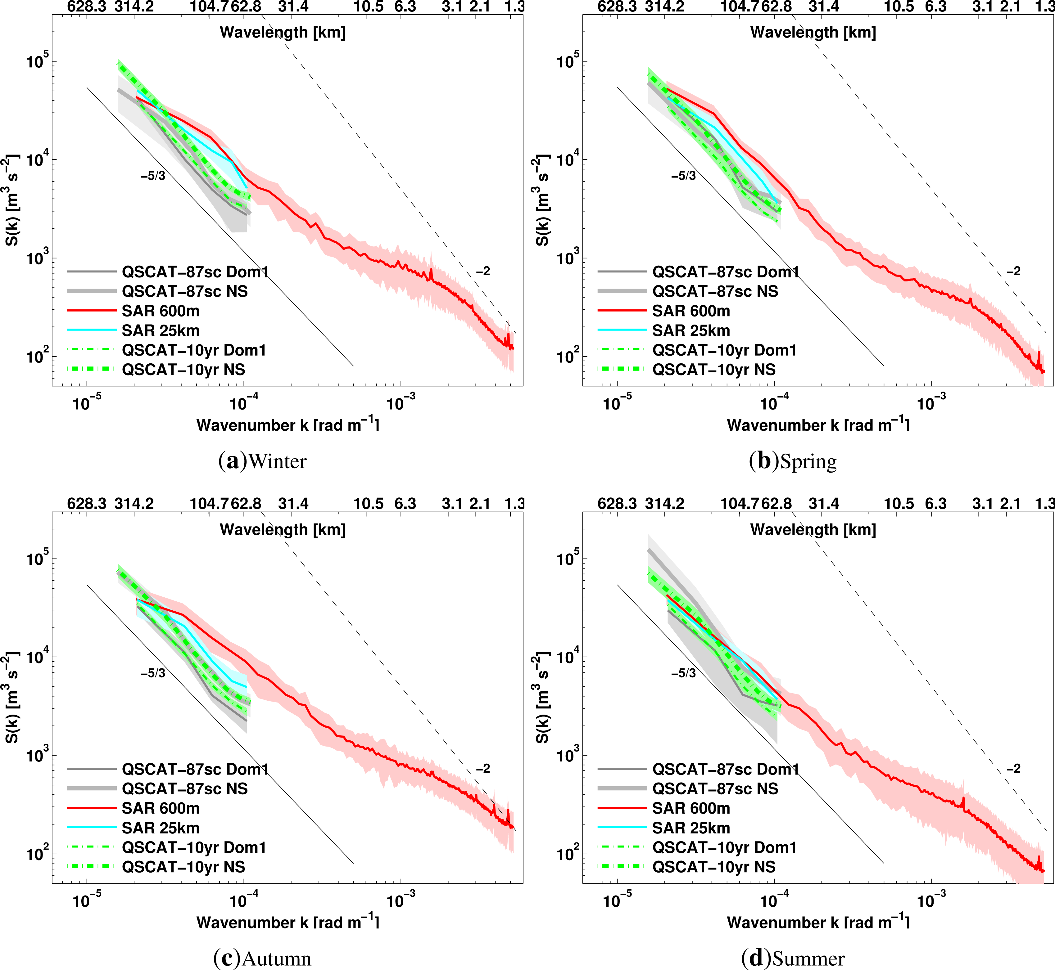
The seasonal spectra are computed to evaluate the seasonal variability (if any) and any potential impact of the small seasonal sample size. Initially, we examine the existence of any seasonal pattern in the QuikSCAT and ENVISAT ASAR sets of 87 scenes through the averaged power spectra as functions of wavenumber k (bottom axis) and wavelength (top axis) in a log-log scale, shown in
Figure 4 along the meridional direction and in
Figure 5 along the zonal direction. The standard deviation associated with each averaged spectrum is shown as a shaded area bounded by the S(k) ± 1
σ curves. A slight decrease in the SAR spectral density levels during summer both along the meridional and zonal directions is noted, especially for the smallest wavenumbers and the
σ values are larger compared to other seasons. This may be an artifact of the sample size as the number of scenes used for the estimation of the seasonal spectra varies between seasons (
Table 1).
The seasonal SAR spectra always show higher spectral density levels compared to the QuikSCAT of the same sample size (gray lines), even for the same resolution, i.e., SAR 25 km (cyan) and QuikSCAT (gray). This difference is larger along the zonal rather than the meridional direction, which can be explained by the small domain size and the errors it may introduce in the QuikSCAT computed spectra. This is also supported by the largest standard deviations estimated for the spectra along the zonal direction.
The impact of the sample size on the seasonal spectra is examined by inspecting the QuikSCAT spectra from the 87 and 5,626 wind maps (gray solid and green dashed lines). In contrast to what
Figure 3 depicts, the sample size has a noticeable impact. Average spectra show different energy levels, and
σ values are higher for the 87-scene dataset compared to the 5,626-scene one. As
Table 1 shows, the 87 wind scene dataset does not allow more than 25 scenes per season. Especially during summer, this number is lower than for the other seasons. It is evident that such a low number of scenes is not sufficient to reproduce the long-term spectral behavior.
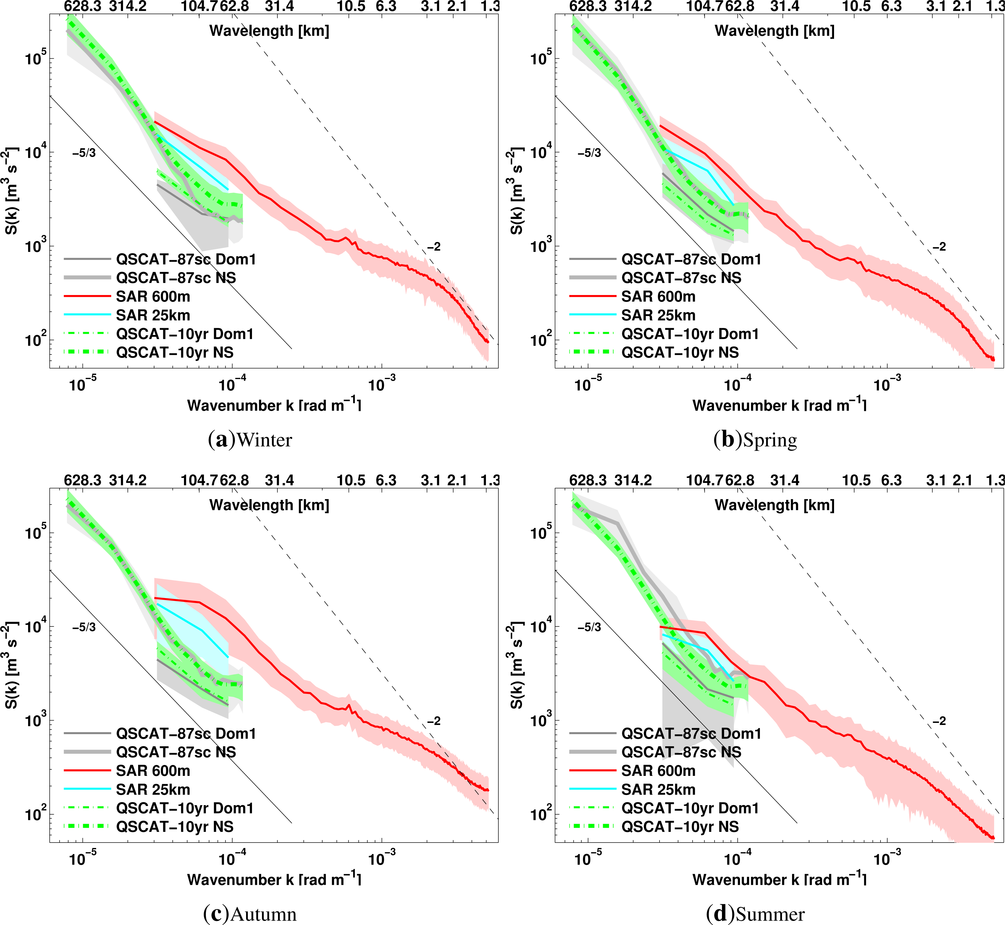
Results inter-comparing the seasonal spectra from the QuikSCAT 10-year archive (
Figure 6) clearly demonstrate the almost non-existent seasonal variability. Average spectra as a function of wavenumber k (bottom axis) and wavelength (top axis) in a log-log scale show that, along the meridional direction and the North Sea domain (thick lines), no significant difference in the spectral density level is identified between spring and autumn (green, red and cyan). There is a small reduction of spectral density levels occurring mostly during summer and for the larger resolvable wavenumbers. Winter spectra (black lines) show slightly higher spectral densities. For the Dom1 (thin lines), between spring and autumn (green, red and cyan), a slight difference is noted for length scales smaller than 90 km. Winter spectra (black) show slightly larger spectral density levels compared to the other seasons. The shaded areas of lighter color are defined by the S(k) ± 1
σ curves and indicate very small standard deviation values for all computed spectra.
Along the zonal direction and the North Sea domain (thick lines), the difference in the QuikSCAT spectral density between winter and the other seasons is even smaller than that along the meridional direction; it can be mostly identified for length scales smaller than 150 km, where the σ values are larger. When Dom1 is examined (thin lines), a clear stratification of the spectra is observed, with winter showing the highest spectral density, followed by autumn, summer and spring, while σ values are significantly larger, especially for summer. This finding strengthens the hypothesis regarding the uncertainties in QuikSCAT spectra for Dom1 along the zonal direction, due to the very small west-east dimensions.
5. Discussion
The current study examines the spectral properties of SAR and QuikSCAT retrieved winds and highlights the advantage of higher resolution products for the identification of small scale features. The retrieval of SAR surface winds at different resolutions can be applicable in the context of offshore wind energy resource assessment in coastal areas, where other space-borne sensors fail, for wind turbine wake studies and to identify finer scale features. For example, the two-dimensional spectral analysis performed on an ASAR retrieved wind scene obtained over the same area as Dom1 in our study showed that the wavelength of the most energetic features was in the range of 5–6 km, and they were recognized as potential atmospheric boundary layer rolls [
21]. Moreover, since wind information from space-borne radars is used for resource assessment, the spectral properties of the derived product aid our understanding of the wind statistics, in terms of mean values and wind distributions. In addition, through the density level, spectra reveal information regarding the wind distribution, as lower levels signify a lack of higher wind speeds represented in the satellite wind products.
The range of resolvable wavenumbers varies depending on the sensor, the resolution of the product and the size of the domain. The power spectrum over a wavenumber range shows the energetic contribution of processes at corresponding length scales. As energy decays with increasing wavenumber, the rate of this decay is represented by the spectral slope. Therefore, the power spectrum and its decay characteristics over a range of wavenumbers provide information regarding the resolvable length scales and, thus, the effective resolution of, in this case, the satellite wind products. In the case of space-borne sensors with spatial resolutions ranging from 600 m to 25 km, the length scales involved extend from the micro- (up to 2 km) to the meso- and synoptic scale (up to 2,000 km). The estimated power spectra correspond to scales ranging between 800 km and 1.2 km. QuikSCAT spectral slopes for wavelengths below 300 km can be affected by “shot noise” in the satellite wind direction [
22], and this has to be taken into account, particularly for small domain dimensions.
In the present study, we select a domain (Dom1) where a sufficient amount of overlapping WSM SAR images is available, covering an area known for its offshore wind farm installations. The size of Dom1 might have an impact on the QuikSCAT-derived spectra, due to the few available spectral nodes; thus, QuikSCAT spectra for the North Sea area are also presented. The impact of the domain size is therefore demonstrated through the spectral density levels. The results shown in this study are not independent of the domain dimensions, as a domain size larger than the North Sea would likely reveal even more synoptic scales and, therefore, potentially exhibit even higher spectral density levels.
Our study reveals QuikSCAT slopes very close to the −5/3 law for length scales between 600 and 60 km. The −5/3 law has been reported to fit spectral decays for length scales smaller than 400 km [
8]. This is generally in agreement with our findings. Higher slopes than our findings have also been reported, but for products with lower resolution and for higher wavenumbers, which generally fits with the theory. For the mid-latitude regions of the Pacific Ocean and for resolvable length scales between 200 and 2,200 km, approximately a k
−2.2 dependence of all zonal, meridional and kinetic energy spectra computed from SASS scatterometer winds with a 50-km resolution was reported [
9]. QuikSCAT swath winds revealed slopes ranging from −2.2 to −2.4 that were computed for length scales between 100 and 1,700 km [
11].
Our study shows that SAR slopes estimated for the range ∼300–∼1 km were generally flatter than the −5/3 law, varying from −0.99 to −1.5. A study using a single SAR scene from ERS and retrieved winds at a 200-m resolution, after averaging of pixels, reported a slope ranging from −1.6 to −1.1 for length scales between 100 and 2 km, while for scales smaller than 2 km, a strong influence of the speckle was noted [
15]. This is in agreement with our findings for similar length scales, but our highest SAR resolution is coarser than that reported in [
15].
In principle, a two-dimensional FFT analysis can be performed. However, in this study, we attempt to investigate the spectral properties of different satellite retrieved wind products, for which one-dimensional spectra are adequate. The unequal dimensions of the domain Dom1 in which QuikSCAT and SAR winds overlap poses a technical difficulty, but such an investigation is considered for a future study. From the literature, it becomes clear that different studies adopted different techniques regarding the spectral investigations. A standardized technique regarding spectral analysis of satellite winds is desirable with best practices regarding the treatment of the data, and it is considered as an outlook for the future.
QuikSCAT data can be found from many sources and processed in different manners, with potentially different spectral characteristics. A study on the verification of scatterometer winds has shown differences between the spectra of QuikSCAT 25-km products processed at two different centers [
20]. It is beyond the scope of this study to further examine potential differences between the QuikSCAT products. Nonetheless, it is relevant for a future study to examine the spectral properties from different QuikSCAT products, such as QuikSCAT L2, and other scatterometers, e.g., ASCAT, which is partly performed in [
20].
SAR winds are retrieved from the commonly available images using different GMFs and processing software, which allows for different selected resolutions. Findings in our study regarding the SAR spectra agree with those in Mourad
et al. [
14] and Horstmann
et al. [
15], where the winds were retrieved with resolutions of 75, 150, 300 and 200 m, correspondingly.
Nonetheless, it was argued in Horstmann
et al. [
15] that the difference in spatial resolution of the SAR winds causes errors in the wind speed, due to speckle noise in the SAR images. They have showed that for resolutions up to 500 m, wind speed retrievals are mainly influenced by this speckle noise, and only above 500 m the actual wind variability dominates. Moreover, they noted that the effect of speckle can start dominating for grid cell sizes smaller than 2 × 2 km. As our SAR 600-m product is very close to the 500-m threshold of spatial resolution, speckle noise may also contaminate the wind retrievals, especially for the very small scales. This may explain the variability in the spectral density of the 600-m product at scales smaller than 2 km.
In addition, as the radar backscatter is relative to the moving ocean surface, surface currents will also have an impact on the retrieved wind. Such effects may not be eliminated by the averaging of grid cells prior to the wind inversion. Oceanic internal waves may also occur, propagating along boundaries between fresh water overlying saline water. A strong current frequently exists along the west coast in Dom1, carrying fresh water from the Elbe river mouth north along the west coast of Denmark. Thus, the potential co-occurrence of both currents and internal waves may also affect the SAR retrieved winds at small scales.
5.1. On the Spatial Resolution
Results presented here indicate that SAR winds, retrieved with various resolutions ranging from 600 m to 25 km, are advantageous for the description of small-scale phenomena and provide information for the energy exchange between the meso- and micro-scales. The effective resolution of the examined satellite products shows that only limited ranges can be studied using certain types of retrieved wind products. For both the QuikSCAT and SAR products used in this study, the effective resolution seems to be lower than that at which the data are retrieved.
A general decrease of spectral density as the resolution decreases has been identified for the SAR wind scenes. In Mourad
et al. [
14], it was also shown that spectra from a single SAR scene processed at 75-, 150- and 300-m resolutions show decreasing spectral density as the resolution decreases. They also found different decay rates between the spectra, especially for very small spatial scales, which was attributed to potential fluctuations in the SAR imagery. These fluctuations were attributed to the variation of the wind, complicated scattering and surface-induced fluctuations, and an averaging to at least a few hundred meters prior to the wind retrieval was advised, in order to smooth out such small-scale variations.
This study finds that SAR spectral slopes are flatter compared to QuikSCAT slopes, even for the same resolution. Such tendencies in slope variations reported by Patoux and Brown [
11] were considered an indication that the smaller scales carry more energy and result in a flatter spectrum. Since the smaller scales are better represented in the SAR products, this can explain their flatter spectral slopes. A study using two different QuikSCAT gridded products from Florida State University and the Jet Propulsion Laboratory reported reduced variance of the gridded product compared to the swath winds, which was attributed to the smoothing effect caused by the interpolation schemes used to produce the gridded L3 data [
19]. In our study, the RSS QuikSCAT gridded product is used, but a similar impact of the interpolation scheme could cause a reduced variance, which would manifest in the QuikSCAT spectra, possibly causing part of its observed discrepancy with the SAR 25-km spectra.
Satellite wind scenes are considered advantageous to modeled winds in terms of their higher effective spatial resolution, as they are not affected by the numerical procedures that cause smoothing effects [
7]. Studies have shown kinetic energy deficiencies of modeled winds when compared to ship measurements [
23], the ERS scatterometer [
12,
24] and QuikSCAT [
20,
25]. Such findings, along with findings from the current study regarding the spectral characteristics of SAR winds, highlight the added qualities that satellite winds can offer to numerical models through data assimilation and model validation.
QuikSCAT offers long temporal and spatial coverage at a relatively low resolution compared to SAR. This study demonstrates the possibility of processing SAR winds with a resolution similar to QuikSCAT, thus rendering the merging of satellite observations possible in order to generate a combined dataset that can increase the temporal coverage of near-surface winds for particular studies, such as wind resource assessment.
When comparing the spectral density levels and resolvable length scales of ASAR and QuikSCAT retrieved winds, the differences of the two sensors in terms of operating frequency and sensor characteristics should be considered. Backscatter from strong scatterers, for example, offshore wind farms in Dom1, can influence the SAR retrieved winds. Such an effect could ideally be removed prior to the wind inversion and can be a suggested “good practice” for spectral analysis. Rain effects are removed from the QuikSCAT spatial series, as rain is a strong scatterer for the Ku band. In addition, it modulates the ocean surface, resulting in rougher surfaces and potentially higher backscatter. QuikSCAT has a rain-flag, which allows for filtering of rain contaminated retrievals. For the C-band, where ASAR operates, the impact of rain is limited, but the rougher ocean surface may also result in stronger backscatter.
Microwave radars provide wind information from the radar backscatter through a GMF, which is calibrated based on certain wind speed ranges; depending on the operational frequency of the radar instrument, different GMFs are used. As such, the very low and high winds are typically absent from space-borne observations, and a part of the arising difference in spectral density levels between QuikSCAT and ASAR can be attributed to differences in the resolvable wind speed range.
5.2. On the Sample Size
Investigations regarding the impact of the sample size showed that, at least for QuikSCAT, no statistically significant differences in the spectra are identified between 87 and more than 5,000 wind scenes. Slope differences between the two datasets (87 vs. 5,626 scenes) are in the range of 0.02–0.09 along the meridional direction, independent of domain size. Along the zonal direction and for the same domain size, slope differences due to the sample size are also very small. Only when the different domains are inter-compared are the slope differences along the zonal direction higher, and this is due to the very small west–east dimension of Dom1.
In agreement with our findings, Xu
et al. [
22] reported a slope difference generally smaller than 0.06, between two and 10 years of QuikSCAT data, while the seasonal slope difference was smaller than 0.1. Thus, the amount of 87 scenes is considered sufficient to describe the long-term spectral properties, but evidence from the seasonal spectra indicate that a sample size of 25 scenes is not adequate to describe the long-term spectra.
5.3. On the Seasonal Variability
The variability found in the SAR and QuikSCAT spectra computed from 87 scenes has been attributed to the small amount of samples categorized seasonally. Findings in this study for a sufficiently large number of samples, as estimated from more than 5,000 QuikSCAT scenes, showed that given a large enough domain, no statistically significant variability can be identified.
Nonetheless, slightly higher spectral density is identified for the winter period from the seasonal spectra computed using the QuikSCAT 10 year dataset. Larsén
et al. [
26] used long-term measurements from offshore meteorological masts in the same area as the sub-domain Dom1 and reported a non important year-to-year spectral variability. Their estimated seasonal spectra showed higher energy and more pronounced slope transition for the winter period due to stronger baroclinity. This is generally in agreement with our findings considering that the spectral behavior should be consistent in the frequency and wavenumber domains.
As large areas need to be considered for a seasonal scale, the size of the domain holds an important role in the calculation of the seasonal spectra. The spectra computed for the sub-domain Dom1 (
Figure 6,) are rather limited in delivering seasonal information. This is because the large scales are not well-resolved due to a lack of entropy/energy transport from the large scales. Our findings indicate that more pronounced differences arise from the sample and domain size, rather than the seasonal variability.
6. Conclusions
This study examined the spectral characteristics of ENVISAT ASAR and QuikSCAT 10-m winds over the North Sea. The resolution of the different satellite wind products varies from 600 m for SAR to 25 km for QuikSCAT. Spatial scales ranging from 1.2 to ∼800 km are represented.
The spectral density of the SAR products is generally higher than QuikSCAT, even for the same resolution, and SAR surface winds effectively resolve much smaller spatial scales than QuikSCAT. Thus, SAR winds are able to potentially record small-scale features in the ocean-surface and contain higher wind variability (i.e., spectral amplitude). Care must be taken for scales smaller than 2 km, as the effects of speckle can be significant.
QuikSCAT spectral slopes for the mid-latitude region of interest follow the theoretical predicted power law of −5/3 for the meso-scale range. The SAR spectral slopes are flatter compared to the QuikSCAT ones, and the SAR spectral density decreases with decreasing spatial resolution.
The observed seasonal variation in the spectra computed from the 87 scenes is attributed to the small sample size. When the sample size is sufficiently large, i.e., 5,626 scenes, QuikSCAT spectra show higher spectral density for winter compared to the other seasons.
Furthermore, it is demonstrated that the SAR processing at very high resolutions preserves small scale features that are otherwise eliminated through averaging, when the wind retrieval is performed at lower resolutions. Thus, SAR winds can be used to describe the small-scale variability of the oceanic surface winds and can be applicable, in the context of wind energy, for detailed studies, such as wake analysis.


