Polarimetric Parameters for Growing Stock Volume Estimation Using ALOS PALSAR L-Band Data over Siberian Forests

Abstract
:1. Introduction
1.1. Polarimetric SAR in Forestry Applications
1.2. Motivation and Scope
1.3. Theoretical Background
1.3.1. Covariance and Coherency Matrix
1.3.2. Four-Component Decomposition
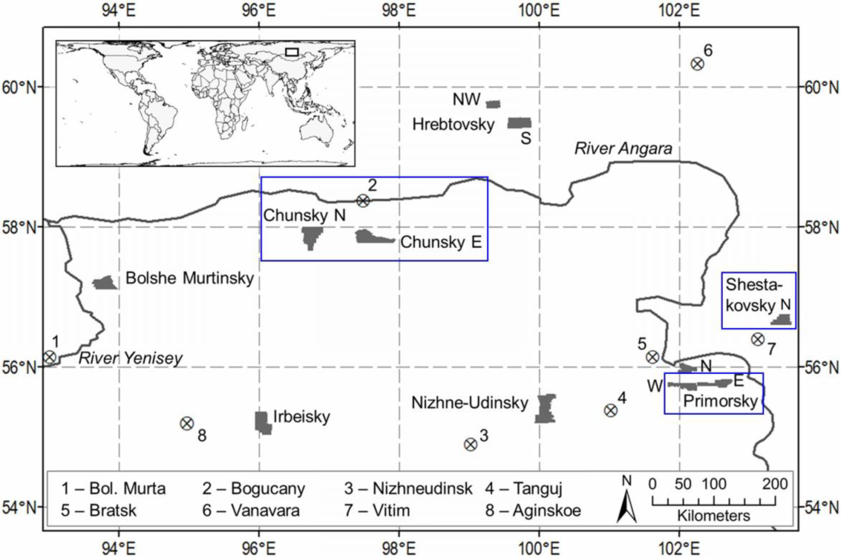
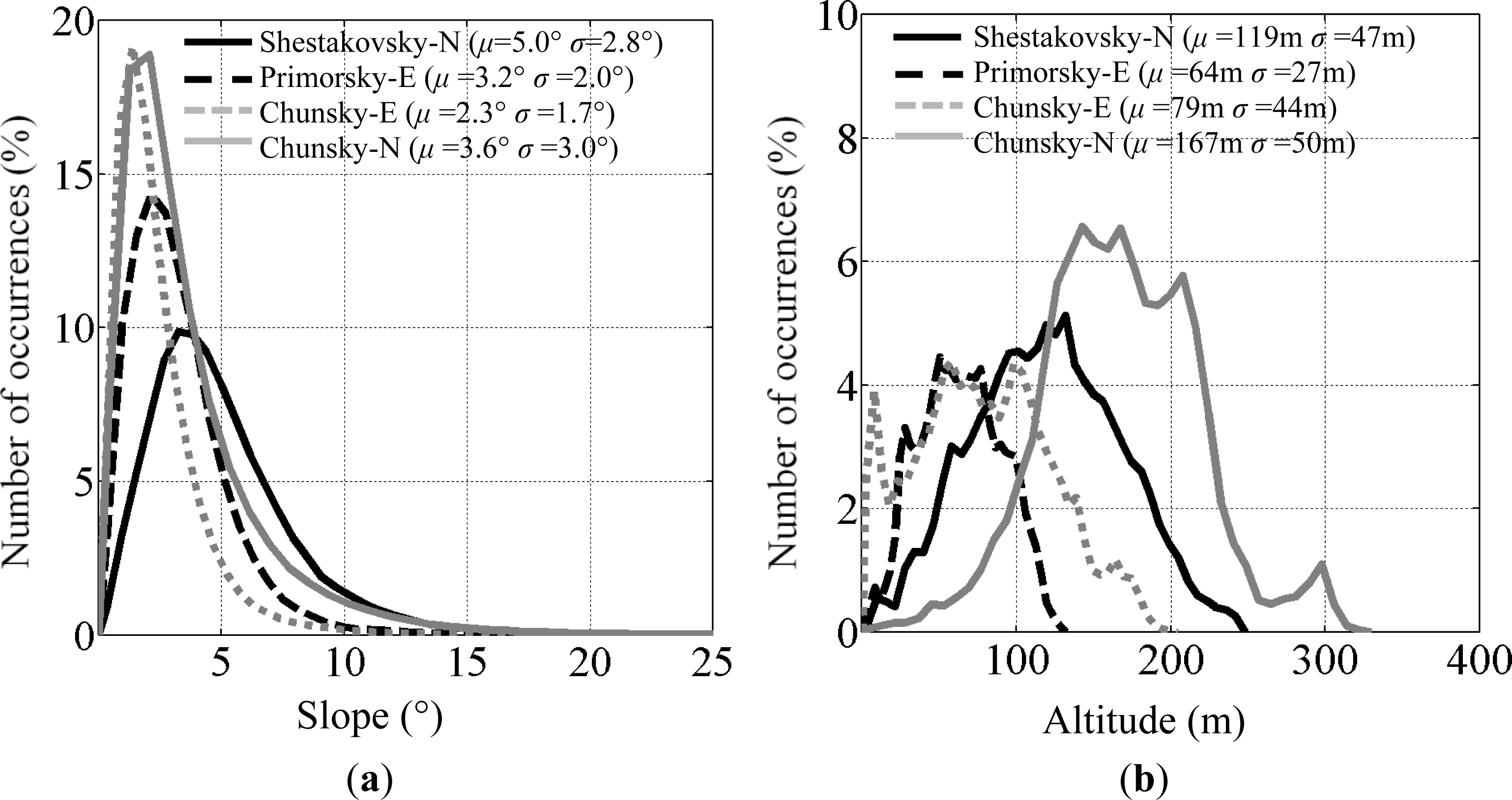
2. Study Area
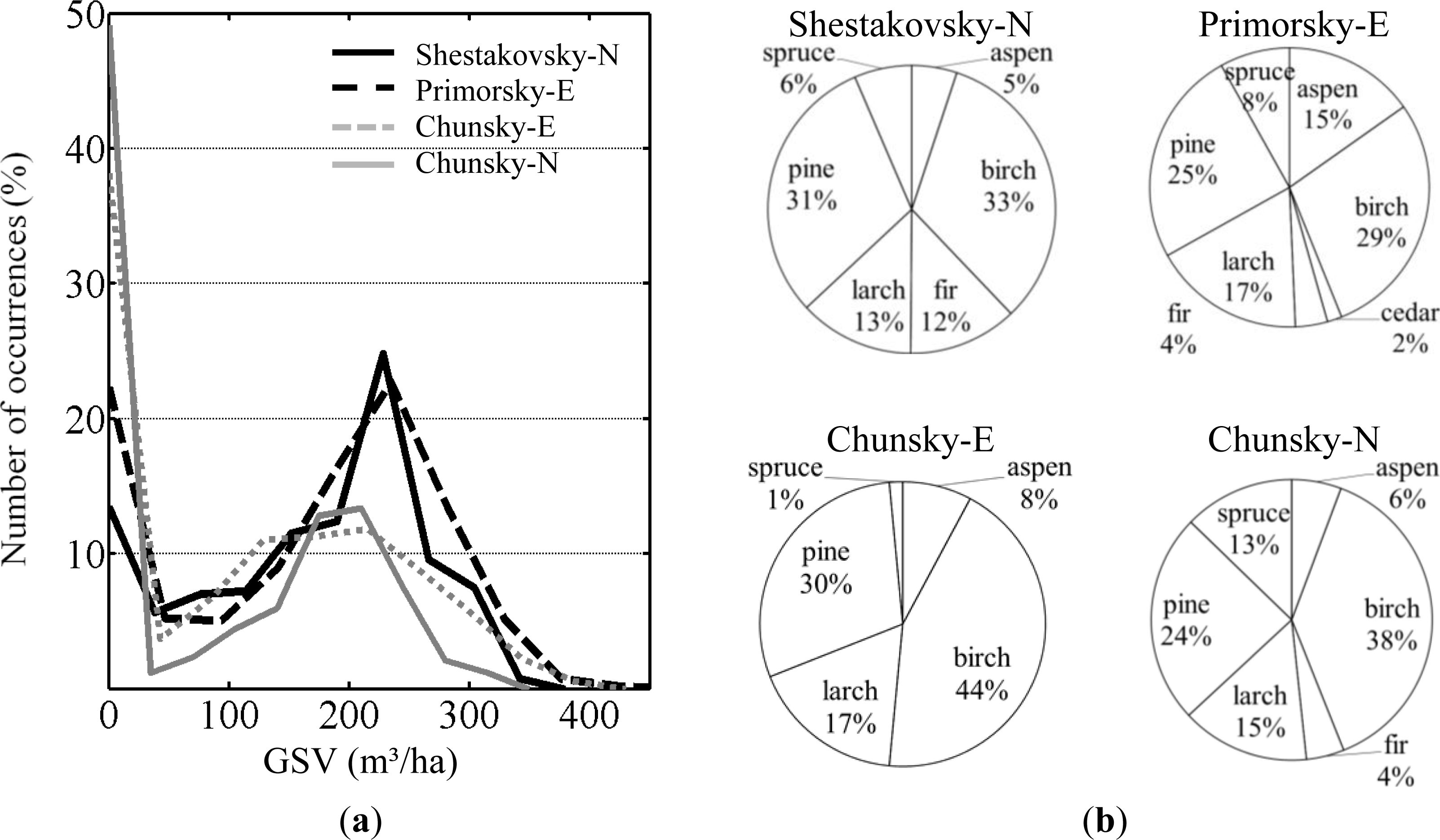
2.1. Shestakovsky
2.2. Primorsky
2.3. Chunsky
3. Data Sets
3.1. Forest Inventory Data
3.2. Weather Data
3.3. PALSAR Data
4. Methods
4.1. SAR Data Pre-Processing
4.2. In-Situ Data Pre-Processing
5. Results
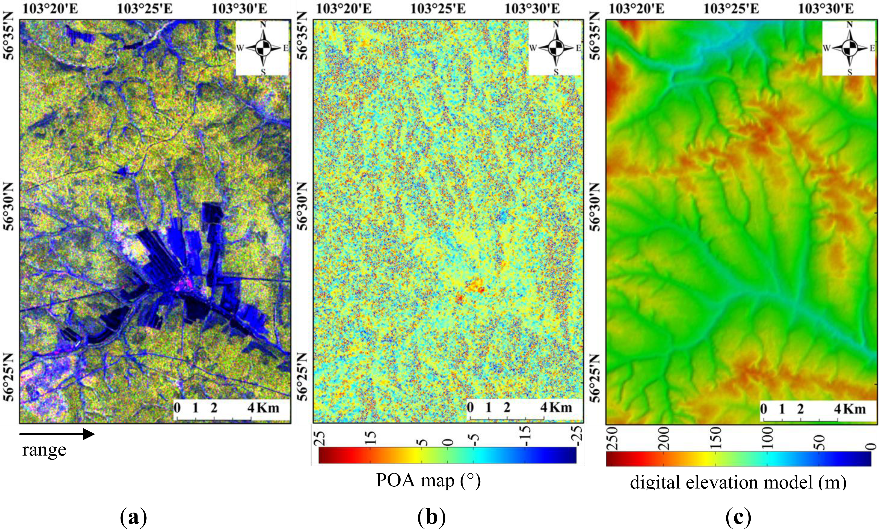
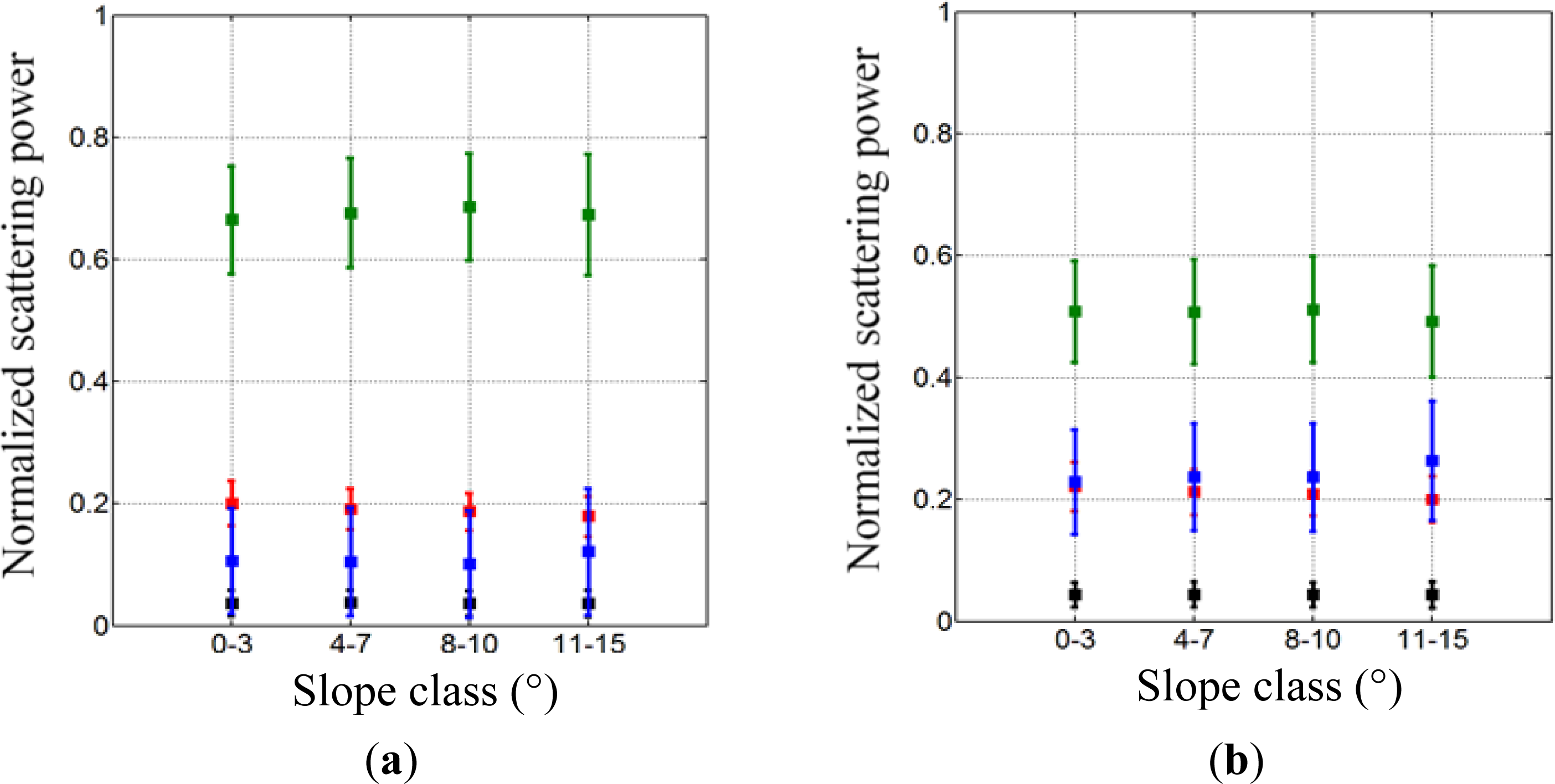
5.1. Impact of Line of Sight (LOS) Rotation
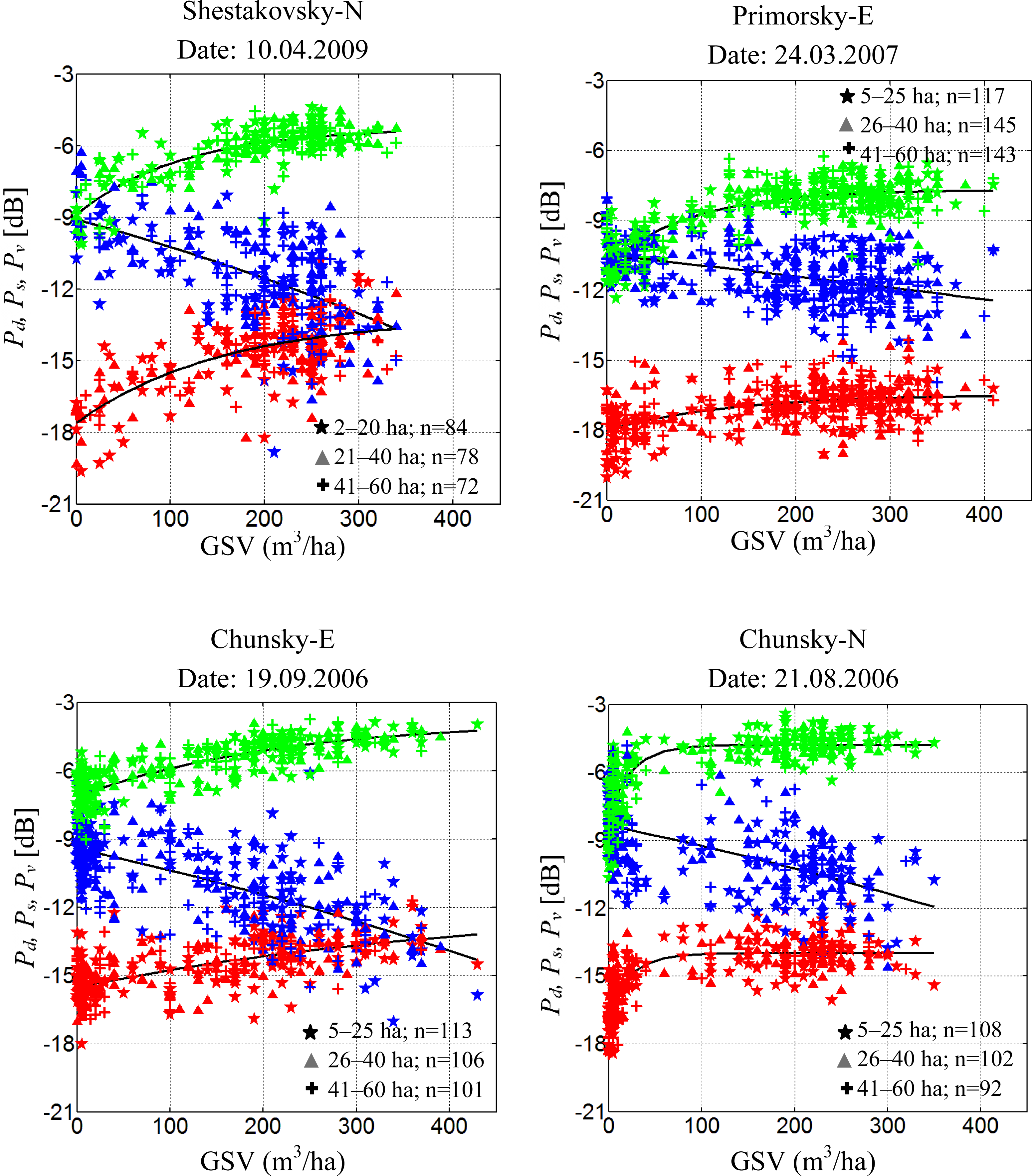
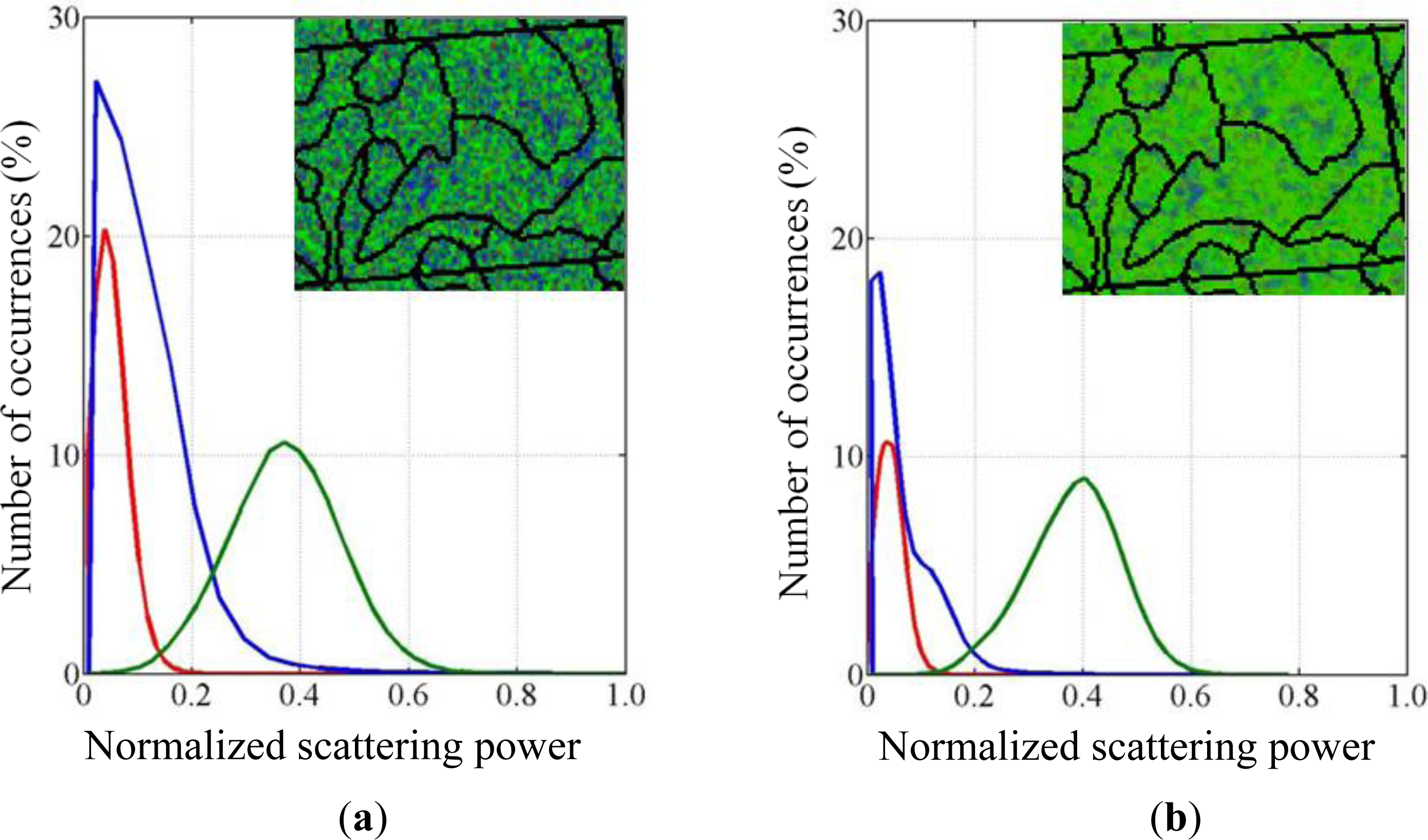
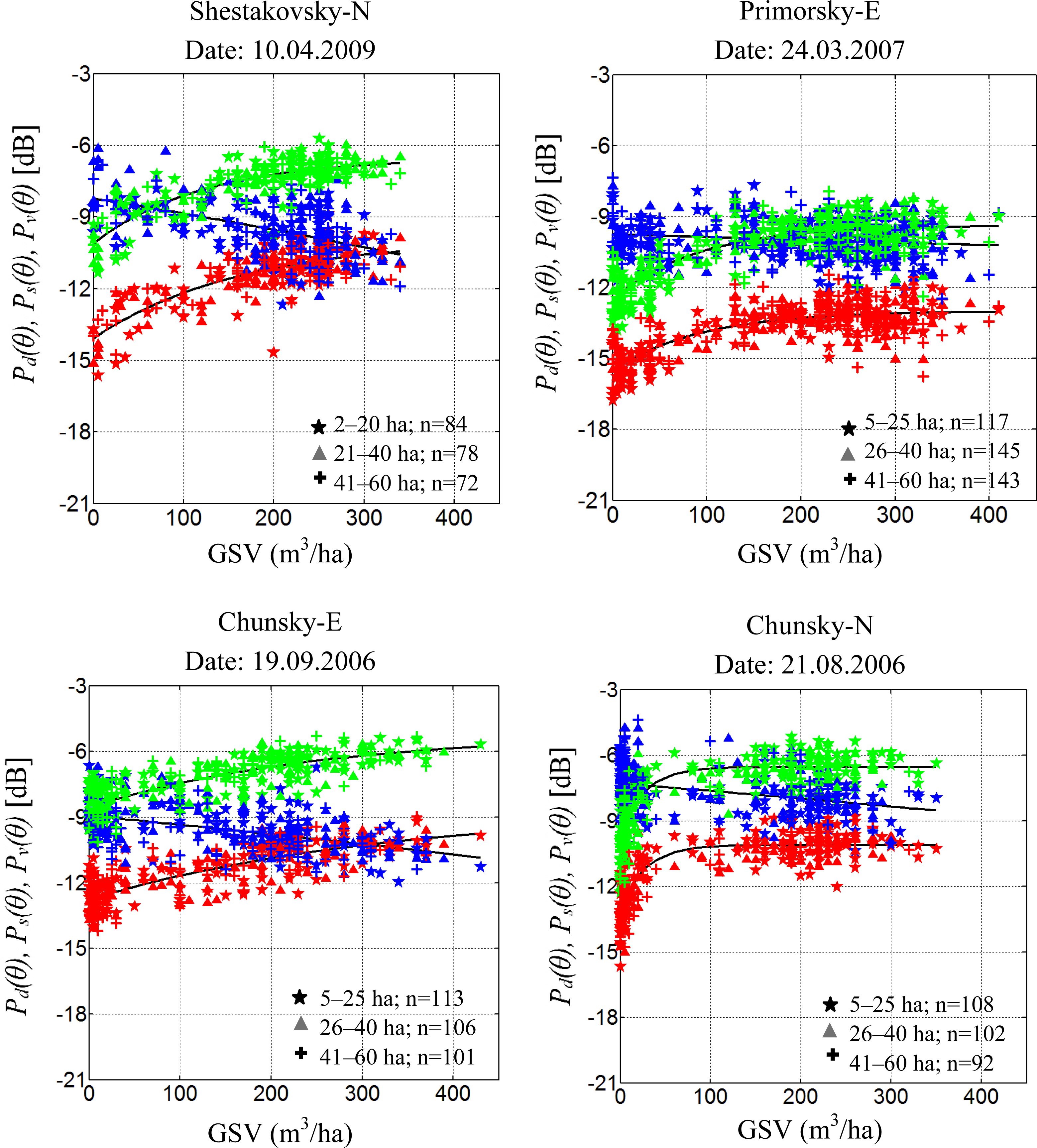
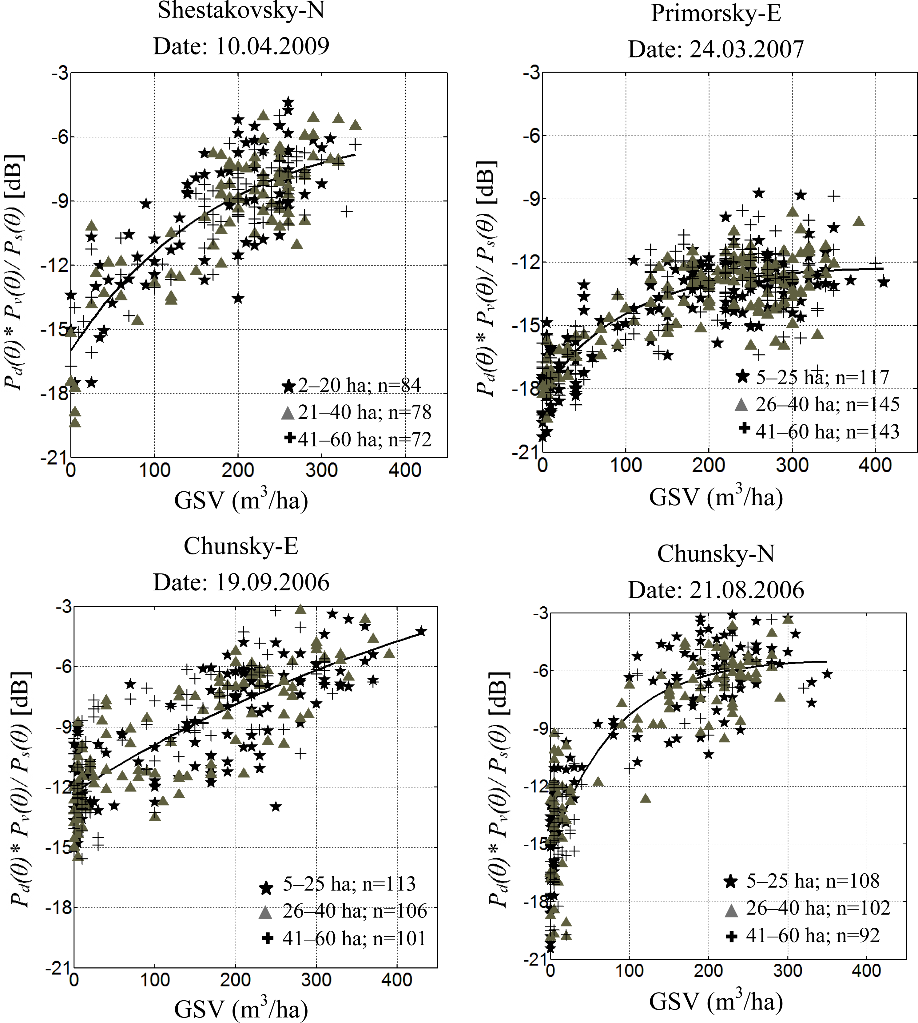
5.2. Growing Stock Volume and Polarimetric Decomposition Powers
5.3. Impact of Weather Conditions on Polarimetric Decomposition Powers
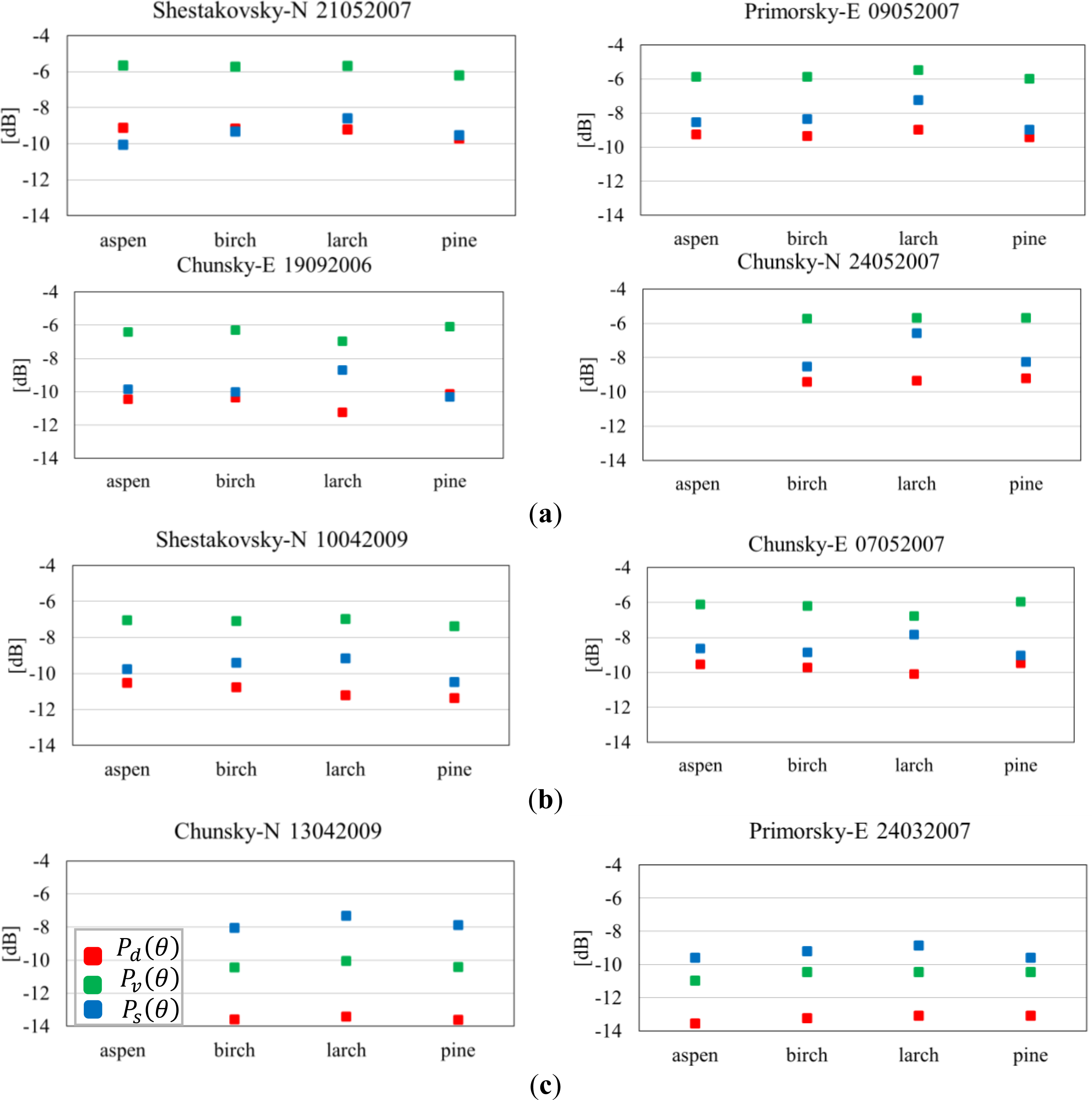
5.4. Impact of Tree Species on Decomposition Powers
6. Discussions
6.1. Growing Stock Volume Estimation Using Polarimetric Information
6.2. Impact of Weather Conditions
6.3. Impact of Tree Species
7. Conclusions
- Double-bounce and volume scattering powers show significant correlation with growing stock volume. The correlation between GSV and surface scattering is found to be inconsistent.
- The importance of the LOS rotation is demonstrated, as the correlation between double-bounce scattering power and GSV could be significantly improved.
- The correlation between polarimetric decomposition parameters and GSV is enhanced if the ratio of volume-to-ground scattering, which is the ratio of volume scattering times double-bounce and surface scattering, is used instead of considering polarimetric decomposition powers separately. The volume-to-ground scattering ratio shows a high sensitivity to GSV. A relatively higher dynamic range is observed for all the investigated areas in Siberia.
- The contribution of decomposition powers over the sparse and dense forest depends on the meteorological conditions. At unfrozen conditions, surface scattering is dominant in sparse forests while in dense forests volume scattering is dominant. During thawing conditions, volume scattering in sparse forests is increased. The scenario is totally different at frozen conditions for dense forest, where the surface scattering power is higher than the volume scattering power.
- The stands dominated by larch species show higher surface scattering power than other tree species. Larch differs from aspen, birch and pine by +2 dB surface scattering power at unfrozen conditions. The double-bounce and volume scattering power for larch was also differed by −1.5 dB and −1.2 dB respectively. At frozen conditions, the impact of tree species on polarimetric decomposition powers is observed to be very small.
Acknowledgments
Conflicts of Interest
References
- Nilsson, S.; Shivdenko, A. Is Sustainable Development of the Russian Forest Sector Possible? IUFRO Occasional Paper No. 11 ISSN 1024–414X; IUFRO Secretariat: Vienna, Austria, 1998; p. 76. [Google Scholar]
- Nilsson, S.; Shivdenko, A.; Stolbovoi, V.; Gluck, M.; Jonas, M.; Obersteiner, M. Full Carbon Account for Russia; International Institute for Applied System Analysis (IIASA): Vienna, Austria, 2000. [Google Scholar]
- Le Toan, T.; Beaudoin, A.; Riom, J.; Guyon, D. Relating forest biomass to SAR data. IEEE Trans. Geosci. Remote Sens 1992, 30, 403–411. [Google Scholar]
- Luckman, A.; Baker, J.; Kuplich, T.M.; Yanasse, C.D.C.F.; Frery, A.C. A study of the relationship between radar backscatter and regenerating tropical forest biomass for space borne SAR instruments. Remote Sens. Environ 1997, 60, 1–13. [Google Scholar]
- Hoekman, D.H.; Quiñones, M.J. Land cover type and biomass classification using AIRSAR data for evaluation of monitoring scenarios in the Colombian Amazon. IEEE Trans. Geosci. Remote Sens 2000, 38, 685–696. [Google Scholar]
- Santoro, M.; Shvidenko, A.; McCallum, I.; Askne, J.; Schmullius, C. Properties of ERS-1/2 coherence in the Siberian boreal forest and implications for stem volume retrieval. Remote Sens. Environ 2007, 106, 154–172. [Google Scholar]
- Lee, J.-S.; Pottier, E. Polarimetric Radar Imaging—From Basics to Applications; CRC Press, Taylor & Francis Group: Boca Raton, FL, USA, 2009. [Google Scholar]
- Van Zyl, J.J. Unsupervised classification of scattering behavior using radar polarimetry data. IEEE Trans. Geosci. Remote Sens 1989, 27, 36–45. [Google Scholar]
- Krogager, E. New decomposition of the radar target scattering matrix. Electron. Lett 1990, 26, 1525–1527. [Google Scholar]
- Cloude, S.R.; Pottier, E. A review of target decomposition theorems in radar polarimetry. IEEE Trans. Geosci. Remote Sens. 1996, 34, 498–518. [Google Scholar]
- Krogager, E.; Madsen, S.N. Comparison of Various Decompositions for Analysis, Interpretation and Classification of Polarimetric SAR Images. Proceedings of European Conference on Synthetic Aperture Radar (EUSAR’96), Königswinter, Germany, 26–28 March 1996.
- Freeman, A.; Durden, S.L. A three-component scattering model for polarimetric SAR data. IEEE Trans. Geosci. Remote Sens 1998, 36, 963–973. [Google Scholar]
- Cloude, S.R.; Pottier, E. An entropy based classification scheme for land applications of polarimetric SAR. IEEE Trans. Geosci. Remote Sens 1997, 35, 68–78. [Google Scholar]
- Ito, Y.; Omatu, S. Polarimetric SAR data classification using competitive neural networks. Int. J. Remote Sens 1998, 19, 2665–2684. [Google Scholar]
- Hellmann, M. Classification of Fully Polarimetric SAR-Data for Cartographic Applications. TU Dresden, Dresden, Germany, 14 April 2000. [Google Scholar]
- Lee, J.S.; Grunes, M.R.; Pottier, E.; Ferro-Famil, L. Segmentation of Polarimetric SAR Images. Proceedings of IEEE International Symposium Geoscience and Remote Sensing (IGARSS’01), Sydney, Australia, 9–13 July 2001.
- Schuler, D.L.; Lee, J.S.; Kasilingam, D.; Nesti, G. Surface roughness and slope measurements using polarimetric SAR data. IEEE Trans. Geosci. Remote Sens 2002, 40, 687–698. [Google Scholar]
- Hajnsek, I.; Pottier, E.; Cloude, S.R. Inversion of surface parameters from polarimetric SAR. IEEE Trans. Geosci. Remote Sens 2003, 41, 727–744. [Google Scholar]
- Thiel, C. Extrahierung Hydrologisch Relevanter Parameter aus Hochaufgelösten Polarimetrischen L-BandSowie Interferometrischen X-Band SAR-Daten. Friedrich-Schiller-Universität Jena, Jena, Germany, 14 July 2004. [Google Scholar]
- Boerner, W.M.; Foo, B.Y.; Eom, H.J. Interpretation of the polarimetric co-polarization phase term in radar images obtained with the JPL airborne L-band SAR system. IEEE Trans. Geosci. Remote Sens 1987, 25, 77–82. [Google Scholar]
- Ulaby, F.T.; Held, D.; Dobson, M.C.; McDonald, K.C.; Senior, T.B.A. Relating polarization phase difference of SAR signals to scene properties. IEEE Trans. Geosci. Remote Sens 1987, 25, 83–92. [Google Scholar]
- Wang, J.R.; Mo, T. The polarization phase differences in orchard trees. Int. J. Remote Sens 1990, 11, 1255–1265. [Google Scholar]
- McNeill, S.; Pairman, D. Stand age retrieval in production forest stands in New Zealand using cand L-band polarimetric radar. IEEE Trans. Geosci. Remote Sens 2005, 43, 2503–2515. [Google Scholar]
- Garestier, F.; Dubois-Fernandez, P.C.; Guyon, D.; Le Toan, T. Forest biophysical parameter estimating using L-band and P-band polarimetric SAR data. IEEE Trans. Geosci. Remote Sens 2009, 47, 3379–3388. [Google Scholar]
- Baker, J.R.; Luckman, A.J. Microwave observations of boreal forests in the NOPEX area of Sweden and a comparison with observations of a temperate plantation in the United Kingdom. Agric. For. Meteorol. 1999, 98–99, 389–416. [Google Scholar]
- Watanabe, M.; Shimada, M.; Rosenqvist, A.; Tadono, T.; Matsuoka, M.; Romshoo, S.A.; Furuta, R.; Nakamura, K.; Moriyama, T. Forest structure dependency of the relation between L-bandσ0 and biophysical parameters. IEEE Trans. Geosci. Remote Sens 2006, 44, 3154–3165. [Google Scholar]
- Goncalves, F.; Santos, J.; Treuhaft, R. Stem volume of tropical forests from polarimetric radar. Int. J. Remote Sens 2011, 32, 503–522. [Google Scholar]
- Kobayashi, S.; Omura, Y.; Sanga-Ngoie, K.; Widyorini, R.; Kawai, S.; Supriadi, B.; Yamaguchi, Y. Characteristics of decomposition powers of L-band multi-polarimetric SAR in assessing tree growth of industrial plantation forests in the tropics. Remote Sens 2012, 4, 3058–3077. [Google Scholar]
- Yamaguchi, Y.; Moriyama, T.; Ishido, M.; Yamada, H. Four-component scattering model for polarimetric SAR image decomposition. IEEE Trans. Geosci. Remote Sens 2005, 43, 1699–1706. [Google Scholar]
- Ranson, K.J.; Sun, G. An evaluation of AIRSAR and SIR-C/X-SAR images for mapping northern forest attributes in Maine, USA. Remote Sens. Environ 1997, 59, 203–222. [Google Scholar]
- Intergovernmental Panel on Climate Change. Volume 4: Agriculture, Forestry and Other Land Use. In IPCC Guidelines for National Greenhouse Gas Inventories; Institute for Global Environmental Strategies: Hayama, Japan, 2006.
- Wagner, W.; Luckman, A.; Vietmeier, J.; Tansey, K.; Balzter, H.; Schmullius, C.; Davidson, M.; Gaveau, D.; Gluck, M.; Le Toan, T.; et al. Large-scale mapping of boreal forest in SIBERIA using ERS tandem coherence and JERS backscatter data. Remote Sens. Environ 2003, 85, 125–144. [Google Scholar]
- Schmullius, C.; Baker, J.; Balzter, H.; Davidson, M.; Eriksson, L.; Gaveau, D.; Gluck, M.; Holz, A.; Letoan, T.; Luckman, A.; et al. SIBERIA—SAR Imaging for Boreal Ecology and Radar Interferometry Applications; Final Report; Contract No. ENV4-CT97-0743-SIBERIA; Centre for Earth Observations: Jena, Germany, 2001. [Google Scholar]
- Balzter, H.; Talmon, E.; Wagner, W.; Gaveau, D.; Plummer, S.; Yu, J.J.; Quegan, S.; Davidson, M.; Le Toan, T.; Gluck, M.; et al. Accuracy assessment of a large-scale forest cover map of central Siberia from synthetic aperture radar. Can. J. Remote Sens 2002, 28, 719–737. [Google Scholar]
- Eriksson, L.; Santoro, M.; Wiesmann, A. Multitemporal JERS repeat-pass coherence for growing stock volume estimation of Siberian forest. IEEE Trans. Geosci. Remote Sens 2003, 41, 1561–1570. [Google Scholar]
- Thiel, C.J.; Thiel, C.; Reiche, J.; Leiterer, R.; Santoro, M.; Schmullius, C. Polarimetric PALSAR SAR Data for Forest Cover Mapping in Siberia. Proceedings of First Joint PI Symposium of ALOS Data Nodes for ALOS Science Program, Kyoto, Japan, 19–23 November 2007.
- Thiel, C.J.; Thiel, C.; Schmullius, C. Operational large-area forest monitoring in Siberia using ALOS PALSAR summer intensities and winter coherence. IEEE Trans. Geosci. Remote Sens 2009, 47, 3993–4000. [Google Scholar]
- Israelsson, H.; Ulander, L.M.H.; Askne, J.L.H.; Fransson, J.E.S.; Frölind, P.-O.; Gustavsson, A.; Hellsten, H. Retrieval of forest stem volume using VHF SAR. IEEE Trans. Geosci. Remote Sens 1997, 35, 36–40. [Google Scholar]
- Cloude, S.R.; Papathanassiou, K.P. Three-stage inversion process for polarimetric SAR interferometry. Proc. Inst. Elect. Eng. Radar Sonar Navig 2003, 150, 125–134. [Google Scholar]
- Praks, J.; Kugler, F.; Papathanassiou, K.P.; Hajnsek, I.; Hallikainen, M. Height estimation of boreal forest: Interferometric model-based inversion at L- and X-band versus HUTSCAT profiling scatterometer. IEEE Trans. Geosci. Remote Sens. Lett 2007, 4, 466–470. [Google Scholar]
- Neumann, M.; Saatchi, S.S.; Ulander, L.M.H.; Fransson, J.E.S. Assessing performance of L- and P-band polarimetric interferometric SAR data in estimating boreal forest above-ground biomass. IEEE Trans. Geosci. Remote Sens 2012, 50, 714–726. [Google Scholar]
- Federal Forest Service of Russia (FFSR). Manual of Forest Inventory and Planning in Forest Fund of Russia, Part 1; FFSR: Moscow, Russia, 1995. [Google Scholar]
- Weather Underground. Available online: www.wunderground.com(accessed on 7–8 June 2010).
- Shimada, M.; Isoguchi, O.; Tadono, T.; Isono, K. PALSAR radiometric and geometric Calibration. IEEE Trans. Geosci. Remote Sens 2009, 47, 3915–3932. [Google Scholar]
- Lee, J.S.; Grunes, M.R.; de Grandi, G. Polarimetric SAR speckle filtering and its implication for classification. IEEE Trans. Geosci. Remote Sens 1999, 37, 2363–2373. [Google Scholar]
- Freeman, A. Calibration of linearly polarized polarimetric SAR data subject to Faraday rotation. IEEE Trans. Geosci. Remote Sens 2004, 42, 1617–1624. [Google Scholar]
- Lee, J.S.; Ainsworth, T.L. The effect of orientation angle compensation on coherency matrix and polarimetric target decomposition. IEEE Trans. Geosci. Remote Sens 2011, 49, 53–64. [Google Scholar]
- Fransson, J.E.S.; Smith, G.; Askne, J.; Olsson, H. Stem volume estimation in boreal forest using ERS-1/2 coherence and SPOT XS optical data. Int. J. Remote Sens 2001, 22, 2777–2791. [Google Scholar]
- Santoro, M.; Askne, J.; Smith, G.; Fransson, J. Stem volume retrieval in boreal forests from ERS-1/2 interferometry. Remote Sens. Environ 2002, 81, 19–35. [Google Scholar]
- Rauste, Y. Multi-temporal JERS SAR data in boreal forest biomass mapping. Remote Sens. Environ 2005, 97, 263–275. [Google Scholar]
- Santoro, M.; Cartus, O. STSE BIOMASAR: Validating a Novel Biomass Retrieval Algorithm Based on Hyper-Temporal Wide-Swath and Global Monitoring ENVISAT ASAR Datasets; Final Report; ESA ESRIN Contract No. 21892/08/I-EC; ESA-ESRIN, Centre For Earth Observation: Rome, Italy, 2010. [Google Scholar]
- Yamaguchi, Y.; Sato, A.; Boerner, W.M.; Yamada, H. Four-component scattering power decomposition with rotation of coherency matrix. IEEE Trans. Geosci. Remote Sens 2011, 49, 2251–2258. [Google Scholar]
- Luckman, A.J.; Baker, J.R; Honzák, M.H.; Lucas, R.M. Tropical forest biomass density estimation using JERS-1 SAR: Seasonal variation, confidence limits and application to image mosaics. Remote Sens. Environ 1998, 63, 126–139. [Google Scholar]
- Fransson, J.E.S.; Israelsson, H. Estimation of stem volume in boreal forests using ERS-1 C- and JERS-1 L-band SAR data. Int. J. Remote Sens 1999, 20, 123–137. [Google Scholar]
- Askne, J.; Santoro, M.; Smith, G.; Fransson, J.E.S. Multitemporal repeat-pass SAR interferometry of boreal forests. IEEE Trans. Geosci. Remote Sens 2003, 41, 1540–1550. [Google Scholar]
- Luckman, A.J.; Baker, J.R.; Wegmüller, U. Repeat-pass interferometric coherence measurements of disturbed tropical forest from JERS and ERS satellites. Remote Sens. Environ 2000, 73, 350–360. [Google Scholar]
- Li, Y.; Cao, F.; Hong, W. Limitations in the Polarization Orientation Shift Estimation Using L Band POLSAR Data. Proceedings of 2009 IET International Radar Conference, Gulin, China, 20–22 April 2009.
- Saatchi, S.S.; McDonald, K.C. Coherent effects in microwave backscattering models for forest canopies. IEEE Trans. Geosci. Remote Sens 1997, 35, 1032–1044. [Google Scholar]
- Sun, G.; Simonett, D.S.; Strahler, A.H. A radar backscatter model for discontinuous coniferous forests. IEEE Trans. Geosci. Remote Sens 1991, 29, 639–650. [Google Scholar]
- Pulliainen, J.T.; Kurvonen, L.; Hallikainen, M.T. Multitemporal behavior of L-band and C-band SAR observations of boreal forests. IEEE Trans. Geosci. Remote Sens 1999, 37, 927–937. [Google Scholar]
- Ranson, K.J.; Sun, G. Mapping biomass of a northern forest using multifrequency SAR data. IEEE Trans. Geosci. Remote Sens 1994, 32, 388–396. [Google Scholar]
- Way, J.; Rignot, E.J.M.; McDonald, K.C.; Oren, R.; Kwok, R.; Bonan, G.; Dobson, M.C.; Viereck, L.A.; Roth, J.E. Evaluating the type and state of Alaska taiga forests with imaging radar for use in ecosystem models. IEEE Trans. Geosci. Remote Sens 1994, 32, 353–370. [Google Scholar]
- Kwok, R.; Rignot, E.J.M.; Way, J.; Freeman, A.; Holt, J. Polarization signatures of frozen and thawed forests of varying environmental state. IEEE Trans. Geosci. Remote Sens 1994, 32, 371–381. [Google Scholar]
- Dobson, M.G.; McDonald, K.; Ulaby, F.T. Effects of Temperature on Radar Backscatter from Boreal Forests. Proceedings of IEEE International Symposium Geoscience and Remote Sensing (IGARSS’90), College Park, MD, USA, 20–24 May 1990; pp. 2481–2484.


| Forest Compartments | Acquisition Date | Temperature (°C) | Weather Conditions | ||
|---|---|---|---|---|---|
| Min | Mean | Max | |||
| Shestakovsky-N T-457 F-1130 | 21.05.2007 | 1 | 6 | 14 | 0.2 cm rain the day before (unfrozen, dry) |
| Shestakovsky-N T-457 F-1130 | 10.04.2009 | −7 | 4 | 17 | snowfall at 21:00 h last 2 days no snow; (thaw, wet) |
| Shestakovsky-N T-457 F-1130 | 26.05.2009 | 5 | 6 | 8 | rainfall at 3:00 h and 21:00 h; last 2 days no rain (unfrozen, wet) |
| Primorsky-E T-459 F-1120 | 09.05.2007 | 4 | 7 | 13 | light rain showers at 23:00 h and 00:00 h; last 1 week no rainfall (unfrozen, dry) |
| Primorsky-E T-459 F-1120 | 24.03.2007 | −8 | −3 | −1 | snowfall at 9:00 h last 20 days snowfall(frozen) |
| Primorsky-E T-460 F-1110 | 31.05.2009 | 6 | 17 | 22 | last 3 days 1.6 cm rain (unfrozen, wet) |
| Chunsky-E T-467 F-1160 | 07.05.2007 | −4 | 7 | 15 | rain at 20:00 h; snowfall day before (thaw, wet) |
| Chunsky-E T-467 F-1160 | 19.09.2006 | 8 | 10 | 14 | 0.3 cm rain; 2 days before 1.1cm rained. (unfrozen, wet) |
| Chunsky-N T-468 F-1160 | 06.10.2006 | −4 | −3 | 1 | snowfall; last day 3 cm snow; snow depth 16 cm (frozen) |
| Chunsky-N T-468 F-1160 | 13.04.2009 | −12 | −7 | −1 | snowfall; snow depth 20 cm (frozen) |
| Chunsky-N T-468 F-1160 | 21.08.2006 | 7 | 11 | 14 | 0.15 cm rain at 08:00 h: 2 cm rain last 4 days (unfrozen, wet) |
| Chunsky-N T-468 F-1160 | 24.05.2007 | 3 | 12 | 17 | 3 days before 0.5 cm rain (unfrozen, dry) |
| Shestakovsky-N | Primorsky-E | Chunsky-E | Chunsky-N | |
|---|---|---|---|---|
| Area (km2) | 86 (146) | 170 (326) | 146 (256) | 200 (312) |
| Number of Stands | 234 (412) | 405 (643) | 320 (564) | 302 (587) |
| Slope: min-mean-max (°) | 0.8-5.0-13.2 | 0.9-3.2-12.0 | 0.5-2.3-9.6 | 0.6-3.6-10.0 |
| Stands size: min-mean-max-stdv (ha) | 2-22-60-12 | 5-28-60-13 | 5-25-60-15 | 5-30-60-12 |
| GSV: min-mean-max-stdv (m3/ha) | 0-189-350-36 | 0-187-410-105 | 0-133-430-114 | 0-107-350-106 |
| Slope Class (°) | μ GSV (m3/ha) | σ GSV(m3/ha) | μ POA (°) | σ POA (°) |
|---|---|---|---|---|
| 0–3 | 193 | 78 | ±3.9 | 2.3 |
| 4–7 | 208 | 78 | ±4.3 | 2.7 |
| 8–10 | 205 | 74 | ±4.5 | 2.9 |
| 11–15 | 202 | 87 | ±4.8 | 3.3 |
| Forest Compartments | Dates | Pd | Pd(θ) | Ps | Ps(θ) | Pv | Pv(θ) |
|---|---|---|---|---|---|---|---|
| Shestakovsky-N | 21.05.2007 | 0.26 | 0.70 | −0.72 | −0.61 | 0.70 | 0.73 |
| Shestakovsky-N | 10.04.2009 | 0.67 | 0.79 | −0.56 | −0.50 | 0.76 | 0.78 |
| Shestakovsky-N | 26.05.2009 | 0.31 | 0.71 | −0.71 | −0.61 | 0.75 | 0.76 |
| Primorsky-E | 09.05.2007 | 0.22 | 0.63 | −0.54 | −0.33* | 0.66 | 0.66 |
| Primorsky-E | 24.03.2007 | 0.48 | 0.70 | −0.43 | −0.15* | 0.74 | 0.74 |
| Primorsky-E | 31.05.2009 | −0.15 | 0.46 | −0.54 | −0.37* | 0.58 | 0.61 |
| Chunsky-E | 07.05.2007 | 0.38 | 0.70 | −0.50 | −0.53 | 0.76 | 0.76 |
| Chunsky-E | 19.09.2006 | 0.64 | 0.80 | −0.67 | −0.52 | 0.81 | 0.81 |
| Chunsky-N | 06.10.2006 | 0.16 | 0.56 | −0.65 | −0.60 | 0.65 | 0.67 |
| Chunsky-N | 13.04.2009 | 0.34 | 0.61 | −0.64 | −0.58 | 0.63 | 0.63 |
| Chunsky-N | 21.08.2006 | 0.61 | 0.77 | −0.60 | −0.36* | 0.74 | 0.76 |
| Chunsky-N | 24.05.2007 | 0.49 | 0.69 | −0.68 | −0.62 | 0.72 | 0.73 |
| Forest Compartments | Dates | σ0(dB) | σ− (dB) | GSV − (m3/ha) | r | R2 | SEE | Weather Conditions |
|---|---|---|---|---|---|---|---|---|
| Shestakovsky-N | 21.05.2007 | −12.6 | −3.9 | 177 | 0.85 | 0.70 | 0.07 | Unfrozen, dry |
| Shestakovsky-N | 10.04.2009 | −15.9 | −5.1 | 190 | 0.80 | 0.68 | 0.06 | Thaw, wet |
| Shestakovsky-N | 26.05.2009 | −11.8 | −3.1 | 126 | 0.81 | 0.75 | 0.08 | Unfrozen, wet |
| Primorsky-E | 09.05.2007 | −10.9 | −6.0 | 114 | 0.74 | 0.64 | 0.08 | Unfrozen, dry |
| Primorsky-E | 24.03.2007 | −18.2 | −12.2 | 103 | 0.78 | 0.69 | 0.02 | Frozen |
| Primorsky-E | 31.05.2009 | −10.2 | −5.7 | 101 | 0.70 | 0.55 | 0.13 | Unfrozen, wet |
| Chunsky-E | 07.05.2007 | −11.8 | 1.15 | 594 | 0.78 | 0.61 | 0.07 | Thaw, wet |
| Chunsky-E | 19.09.2006 | −12.3 | 3.1 | 595 | 0.81 | 0.67 | 0.05 | Unfrozen, wet |
| Chunsky-N | 06.10.2006 | −20.3 | −12.2 | 128 | 0.84 | 0.79 | 0.05 | Frozen |
| Chunsky-N | 13.04.2009 | −20.0 | −12.3 | 126 | 0.90 | 0.82 | 0.05 | Frozen |
| Chunsky-N | 21.08.2006 | −15.3 | −5.4 | 82 | 0.87 | 0.81 | 0.07 | Unfrozen, wet |
| Chunsky-N | 24.05.2007 | −15.2 | −6.7 | 80 | 0.85 | 0.80 | 0.08 | Unfrozen, dry |
| Forest Compartments | Aspen | Birch | Larch | Pine | ||||
|---|---|---|---|---|---|---|---|---|
| μ (m3/ha) | σ (m3/ha) | μ (m3/ha) | σ (m3/ha) | μ (m3/ha) | σ (m3/ha) | μ (m3/ha) | σ (m3/ha) | |
| Shestakovsky-N | 267 | 28 | 201 | 23 | 242 | 37 | 259 | 46 |
| Primorsky-E | 290 | 48 | 205 | 26 | 239 | 53 | 278 | 46 |
| Chunsky-E | 266 | 55 | 212 | 24 | 198 | 17 | 302 | 38 |
| Chunsky-N | — | — | 172 | 13 | 225 | 30 | 250 | 52 |
© 2013 by the authors; licensee MDPI, Basel, Switzerland This article is an open access article distributed under the terms and conditions of the Creative Commons Attribution license ( http://creativecommons.org/licenses/by/3.0/).
Share and Cite
Chowdhury, T.A.; Thiel, C.; Schmullius, C.; Stelmaszczuk-Górska, M. Polarimetric Parameters for Growing Stock Volume Estimation Using ALOS PALSAR L-Band Data over Siberian Forests. Remote Sens. 2013, 5, 5725-5756. https://doi.org/10.3390/rs5115725
Chowdhury TA, Thiel C, Schmullius C, Stelmaszczuk-Górska M. Polarimetric Parameters for Growing Stock Volume Estimation Using ALOS PALSAR L-Band Data over Siberian Forests. Remote Sensing. 2013; 5(11):5725-5756. https://doi.org/10.3390/rs5115725
Chicago/Turabian StyleChowdhury, Tanvir Ahmed, Christian Thiel, Christiane Schmullius, and Martyna Stelmaszczuk-Górska. 2013. "Polarimetric Parameters for Growing Stock Volume Estimation Using ALOS PALSAR L-Band Data over Siberian Forests" Remote Sensing 5, no. 11: 5725-5756. https://doi.org/10.3390/rs5115725