Assessing the Performance of a Northern Gulf of Mexico Tidal Model Using Satellite Imagery

Abstract

Tidal harmonic analysis simulations along with simulations spanning four specific historical time periods in 2003 and 2004 were conducted to test the performance of a northern Gulf of Mexico tidal model. A recently developed method for detecting inundated areas based on integrated remotely sensed data (i.e., Radarsat-1, aerial imagery, LiDAR, Landsat 7 ETM+) was applied to assess the performance of the tidal model. The analysis demonstrates the applicability of the method and its agreement with traditional performance assessment techniques such as harmonic resynthesis and water level time series analysis. Based on the flooded/non-flooded coastal areas estimated by the integrated remotely sensed data, the model is able to adequately reproduce the extent of inundation within four sample areas from the coast along the Florida panhandle, correctly identifying areas as wet or dry over 85% of the time. Comparisons of the tidal model inundation to synoptic (point-in-time) inundation areas generated from the remotely sensed data generally agree with the results of the traditional performance assessment techniques. Moreover, this approach is able to illustrate the spatial distribution of model inundation accuracy allowing for targeted refinement of model parameters.

1. Introduction

Accurate simulation of the tides is the foundation for any study involving modeling of coastal hydrodynamics. Developing an accurate tidal simulation provides the basis for validating model skill before incorporating more complex processes such as river inflow, wind, atmospheric pressure, and surface waves. Using this strategy for developing an accurate comprehensive coastal circulation model, the first step is to test the performance of the model in accurately reproducing the local tides.

The assessment of a model’s performance will herein be referred to as its skill [1], where skill is typically measured by comparing model output to observed data. The most basic comparison is to perform a resynthesis of observed harmonic tide constituents. It is relevant to note that such a comparison of harmonic tide constituents is only attainable at constantly submerged locations since the harmonic tide constituents cannot be computed when the location experiences extended dry periods. While the National Oceanic and Atmospheric Administration-National Ocean Service (NOAA-NOS) has standard methods for resolving gaps in the data using a least squares fit [2], harmonic analysis is not possible at some upriver stations where the gage is dry for long periods of time. As such, gages are installed and maintained off of piers or jetties, measure continuous water levels, perform harmonic analysis on those measured water levels and report the harmonic tide constituents [3]. Historical harmonic tide constituents can be obtained from gages situated within a model’s interior, and compared to harmonic tide constituents derived from water level time series computed by the model. In the United States and its territories, this information is available from the National Oceanic and Atmospheric Administration Center for Operational Oceanographic Products and Services (NOAA CO-OPS, http://tidesandcurrents.noaa.gov/). In the event that the subject gage is not maintained by NOAA CO-OPS and/or does not provide harmonic constituents, the historic water level time series can be decomposed [4,5]. One tool for completing this type of analysis is the T_TIDE software package [6].

Additional historical data such as observed water level time series and measured high water marks are also used to validate storm surge models, such as done for model hindcasts in the northern Gulf of Mexico (Westerink et al. [7], Bunya et al. [8] and Dietrich et al. [9]). Comparison to historical high water marks is a limited assessment as it only considers the maximum water level predicted by the model at a given location without providing a skill measure of when the maximum water level occurred. Also, high water mark measurements can be affected by processes such as short wave run-up, as well as by the subjective selection of the actual high water mark elevation [10].

An assessment of model skill that incorporates both spatial and temporal factors is required in order to examine not only the ability of the model to predict water levels at specific locations, but also the ability of the model to predict the spatial extent of inundated areas. This is important for modeling the flooding and drying of tidal flats for ecological studies, projecting the condition of evacuation/access routes during and after major storms, and assessing the availability of estuarine navigational access.

Most, but not all, contemporary coastal circulation models employ a numerical wetting and drying (WD) algorithm to simulate the physics of an advancing or receding flood wave. A review of these algorithms is provided by Medeiros and Hagen [11]. WD is a crucial component of models seeking to simulate the astronomic tide. It has been shown that the flooding and ebbing of the tides within coastal marshes can significantly affect the amplitude and phase of the astronomic tide [12]. WD is also needed to simulate the rate of flood and ebb of non-cyclical events such as storm surge [13]. However, the means to test the performance of WD in large scale distributed models are limited, particularly the prediction of the extent of inundation.

Recent advances in the use of remotely sensed data to detect inundated areas have taken steps toward this end. In particular, studies conducted by Horritt et al. [14] and Chaouch et al. [15] used SAR to detect inundated areas. The method developed by Horritt et al. [14] was tested by Cobby et al. [16] and Mason et al. [17] in river flood scenarios. The primary difference between the method of Horritt et al. [14] and Chaouch et al. [15] is the former computes the inundation extent as a vector feature (line) using a statistical active contour model where the latter computes a raster representation of cells as wet or dry. In addition to using active sensors such as SAR, passive optical sensors such as MODIS and Landsat have also been used to identify inundated areas [18,19]. In this paper, the approach of Chaouch et al. [15], herein referred to as the “synergetic method”, is used to validate a tidal model.

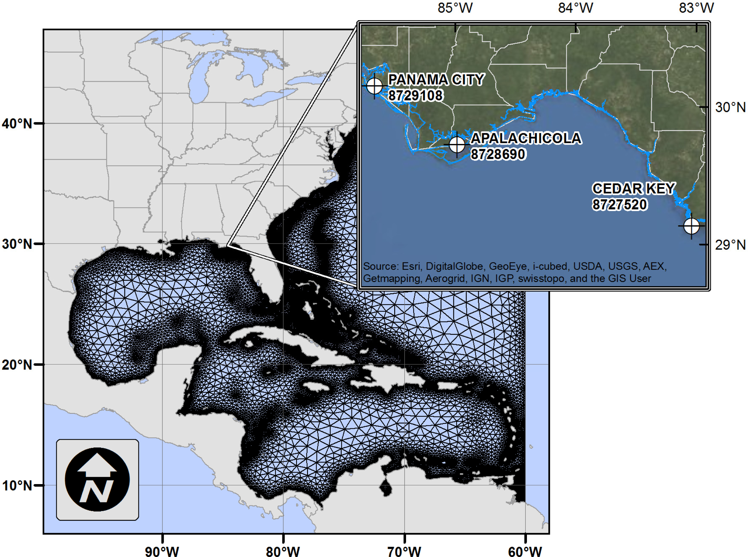
The synergetic method proposed by Chaouch et al. [15] uses a change detection approach to analyze Radarsat-1 imagery, in particular the distribution of the backscatter values. The development of the synergetic method employed a novel approach for identifying the area subject to tidal fluctuations a priori and applying the change detection algorithm within that pre-defined band of land area. Masking out the areas that were either always dry or always wet significantly increased the accuracy of the method. The method was validated synoptically by comparing the predictions of inundated area with historic aerial imagery in the Apalachicola region of the Florida panhandle (location shown in Figure 1). Please note that herein the term synoptic refers to the environmental conditions across a broad area occurring at a specific point in time.

This paper extends the previous study by Chaouch et al. [15] and applies the synergetic method to assess the performance of a tidal model of the northern Gulf of Mexico in simulating coastal inundation. First, the performance of the model at tide gage stations is assessed by harmonic analysis and comparison of model output to time synchronized water level measurements over four separate time periods in the years 2003 and 2004. Then, model performance in coastal regions where both wet and dry conditions occur is assessed by comparing inundated areas generated by the model to inundated areas detected using the synergetic method over four areas within the domain during the same time periods were evaluated for the time series analysis.

2. Tidal Model Description

For tidal calculations, the two-dimensional, depth-integrated ADCIRC code [20,21] was used. ADCIRC solves the shallow water equations in their barotropic form expressed in spherical coordinates [22]. The model is based on the Western North Atlantic Tidal (WNAT) model domain that extends eastward from the 60° west meridian to the North and South American coastlines, incorporating the Atlantic Ocean, Caribbean Sea and the Gulf of Mexico (see Figure 2). In order to produce accurate results, the model boundary must be established well outside the Gulf of Mexico to allow adequate spatial extent for the propagation of nonlinear model physics through the Caribbean Sea, into the Gulf and up to the focus area [23]. Large-scale processes in the Gulf of Mexico such as the Loop Current [24] were not included. 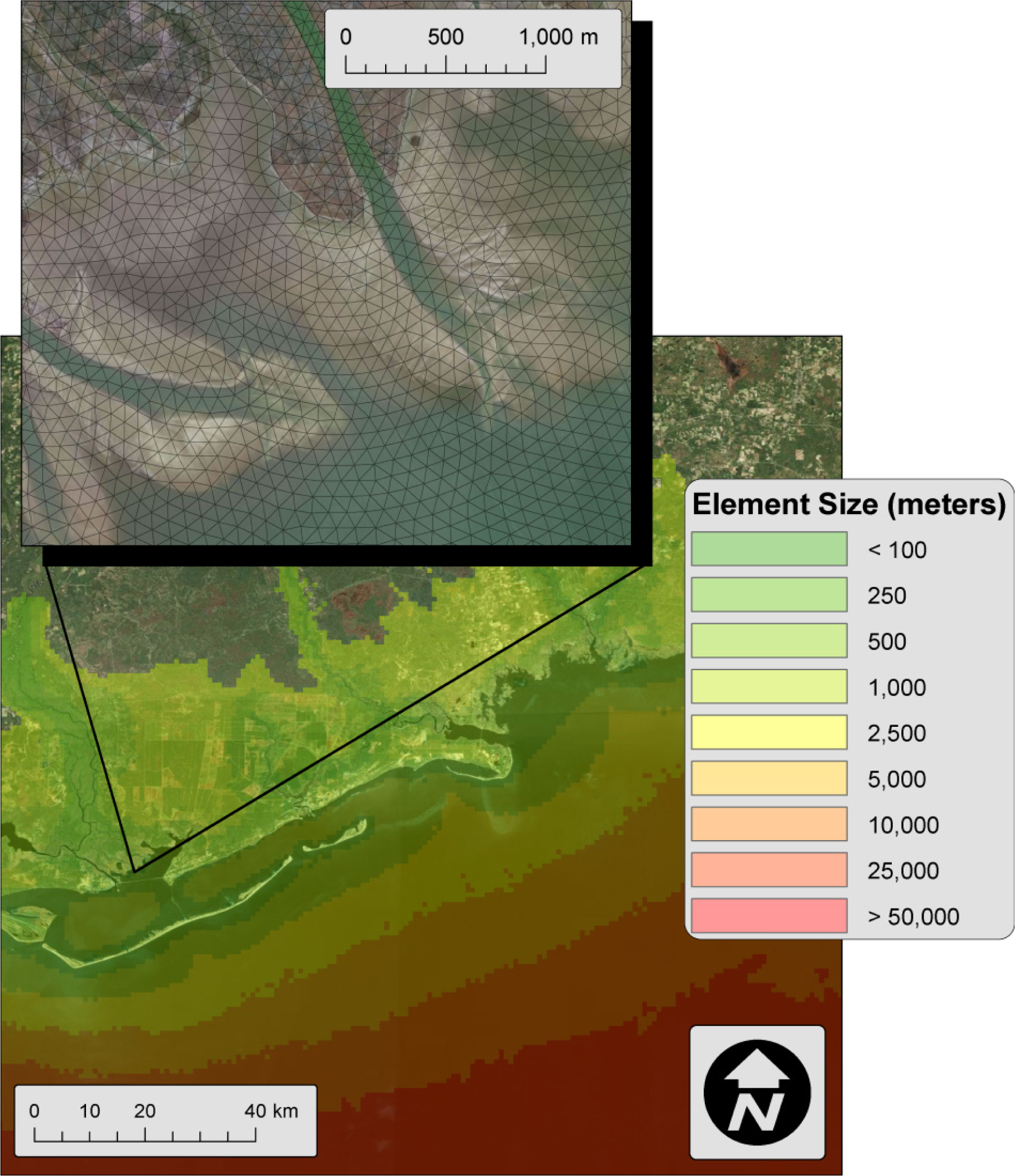The model focused on the Apalachicola area and was constructed as part of a Federal Emergency Management Agency (FEMA) map modernization study of Franklin, Jefferson and Wakulla (FWJ) counties in Florida [25]. This model, herein referred to as FWJ, was selected for its high resolution in the Apalachicola, Florida region with node spacing of 30–50 m in the river channels and bank areas and 250–300 m in the floodplains (see Figure 2). Detailed descriptions of the model development, including the sources of topography, bathymetry, surface roughness parameterization and tidal validation at four stations located in the focus area of the mesh, including Apalachicola, can be found in Coggin et al. [26], Salisbury et al. [27] and Atkinson et al. [10].

For the research conducted herein, the model was forced at the open ocean boundary using 10 tidal constituents (STEADY, K₁, O₁, Q₁, M₂, S₂, N₂, K₂, M₄ and M_6;

Table 1. Dominant tidal constituents at the Apalachicola station.

Constituent Name	Description	Frequency (cycles/h)	Amplitude (m)
K1	Lunar diurnal	0.0418	0.130
M2	Principal lunar semidiurnal	0.0805	0.116
O1	Lunar diurnal	0.0387	0.112
P1	Solar diurnal	0.0416	0.043
S2	Principal solar semidiurnal	0.0833	0.037
Q1	Larger lunar elliptic diurnal	0.0372	0.023
N2	Larger lunar elliptic semidiurnal	0.0790	0.018
K2	Lunisolar semidiurnal	0.0836	0.016

). Eight tidal potential terms were also included (K₁, O₁, P₁, Q₁, M₂, S₂, N₂ and K₂). These terms were derived from the FES.95.2 tidal database [28]. No other forcing such as river inflow, winds or pressures were considered. A one-second time step was used over a 45 day simulation that began with a 10 day ramp up to allow the model to reach steady state. Also, an initial water level adjustment, specific to each simulated time period, was implemented to account for the seasonal steric effects that cause swelling or contraction of the Gulf of Mexico [7]. This adjustment is necessary to account for deviations from mean sea level due to thermal and atmospheric pressure effects that are particularly pronounced in the central northern Gulf of Mexico [29]. For the Apalachicola station, these adjustments range from −10 cm in the winter months to +6.1 cm in the late summer ( http://tidesandcurrents.noaa.gov/sltrends/seasonal.shtml?stnid=8728690).

The periodic boundary forcing and tidal potential terms (amplitude and phase) were unmodified for the simulations used to analyze the resynthesized tides from the model output and historic gage station constituents. For the simulations used to produce water level time series comparisons and the wet/dry output image for comparison to the synergetic method, tidal nodal factors and equilibrium arguments [5] for the boundary forcing and tidal potential terms were adjusted to synchronize the model output with the synergetic method snapshot times discussed in the next section.

3. Model Performance Assessment

The tidal model was evaluated using three methods for skill measure: harmonic analysis, synoptic water level time series and spatial extent of inundation. The first two methods are common in coastal modeling and give insight into model skill at specific locations within the model domain. They are herein referred to as “traditional methods”. The third method is a novel approach that tests not only the model’s ability to capture the astronomic tide at specific locations, but also its ability to accurately predict the spatial extent of inundation at specific points in time. These methods focus on three characteristics of the model: the resolution of the finite element mesh in key areas, the description of the terrain processed by the model, and the wetting and drying algorithm used within the numerical code.

The harmonic analysis was conducted at three NOS tide gage stations within the model domain: Apalachicola, FL 8728690; Panama City, FL 8729108; and Cedar Key, FL 8727520 (see Figure 1). Twenty-three constituents are built in to the ADCIRC model and harmonically analyzed over the final 30 days of a 45 day simulation [30]. These constituents were resynthesized to form the predicted tides at each station. NOS provides 37 harmonic constituents at each station that are derived from decomposing the observed tides over a 19 year tidal epoch ( http://tidesandcurrents.noaa.gov/station_retrieve.shtml?type=Harmonic+Constituents). They were then resynthesized to form the theoretical tides at each station. For brevity, only the eight most dominant constituents in terms of amplitude (excluding the Solar Annual and Solar Semi-Annual) at the Apalachicola station are shown in Table 1 along with their associated frequencies and amplitudes [4,6].

Following Willmott [31], the results of the harmonic analysis were assessed both visually and quantitatively beginning with the model skill measure presented by Warner et al. [1]:

$$\mathit{Skill}=1-\frac{\sum {\left|H_{\mathit{model}}-H_{\mathit{obs}}\right|}^2}{\sum {\left(\left|H_{\mathit{model}}-\overline{H_{\mathit{obs}}}\right|+\left|H_{\mathit{obs}}-\overline{H_{\mathit{obs}}}\right|\right)}^2}$$

(1)

where H_model is the water surface elevation computed by the tidal model at a specific time (meter); H_obs is the observed water surface elevation at a tide gage station (meter); and $\overline{H_{\mathit{obs}}}$ is the mean observed water surface elevation over the comparison period (meter). A skill value approaching unity indicates a well performing model.

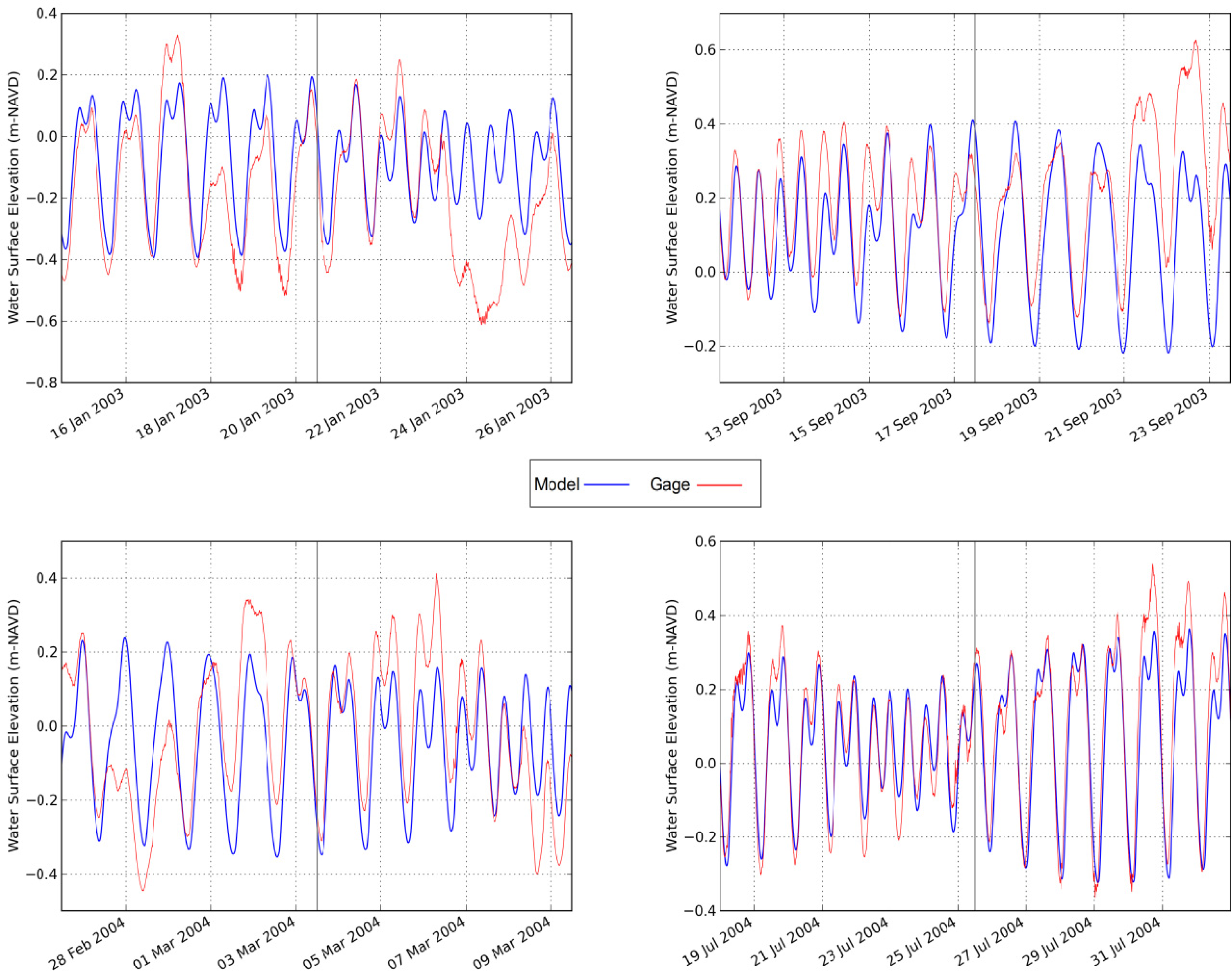
Time series of the water level for the four time periods (see

Table 2. Simulation time period information.

Simulation	Simulation Start	Radarsat-1 Scene	Simulation End
1	21 December 2002	20 January 2003	4 February 2003
2	18 August 2003	17 September 2003	2 October 2003
3	2 February 2004	3 March 2004	18 March 2004
4	25 January 2004	25 July 2004	9 August 2004

) at each of the three stations (Figure 1) were also used to assess the performance of the tidal model. These water level time series were analyzed at the Apalachicola station over the four time periods that coincide with the Radarsat-1 scene acquisition dates. Since only the Apalachicola station lies within both the focus area and Radarsat scene boundary, NOS stations in Panama City and Cedar Key are omitted from this point on. The performance of the model was again assessed visually and also using the model skill measure of Equation (1) over a 15 day period extending from seven days prior to and seven days after the Radarsat-1 scene snapshot time. Furthermore, the root mean square error (RMSE) for both the harmonic analysis and the 15 day water level time series was computed according to the following formula:

$$\mathit{RMSE}=\frac{\sqrt{\sum {\left(H_{\mathit{model}}-H_{\mathit{obs}}\right)}^2}}{N}$$

(2)

where N is the number of observations. The normalized RMSE (NRMSE) was also calculated to account for the tidal range when assessing the impact of an error. The RMSE was normalized using the range of water surface elevations present at the tide gage during the relevant time period as follows:

$$\mathit{NRMSE}=\frac{\mathit{RMSE}}{H_{\mathit{obs}-\text{max}}-H_{\mathit{obs}-\text{min}}}$$

(3)

Lastly, the model performance was assessed based on the areal extent of the inundated area at a specific historic time. Radarsat-1 is an orbital satellite commissioned by the Canadian Space Agency that has a SAR sensor on board. The spatial resolution of the Radarsat-1 imagery used in this study was 25 m. The C-band (5.6 cm wavelength) imagery was acquired in standard mode, with consistent observation geometry. A change detection approach was utilized that compared the SAR backscatter imagery from a scene with very low water to a scene with inundation present. This provided the foundation for an analysis of the backscatter histogram that indicated a break in the distribution of backscatter values corresponding to the threshold between inundated and non-inundated areas. With this threshold established, this technique, termed the synergetic method, could be applied to a variety of settings with good results. Details regarding the development and testing of the synergetic method can be found in Chaouch et al. [15].

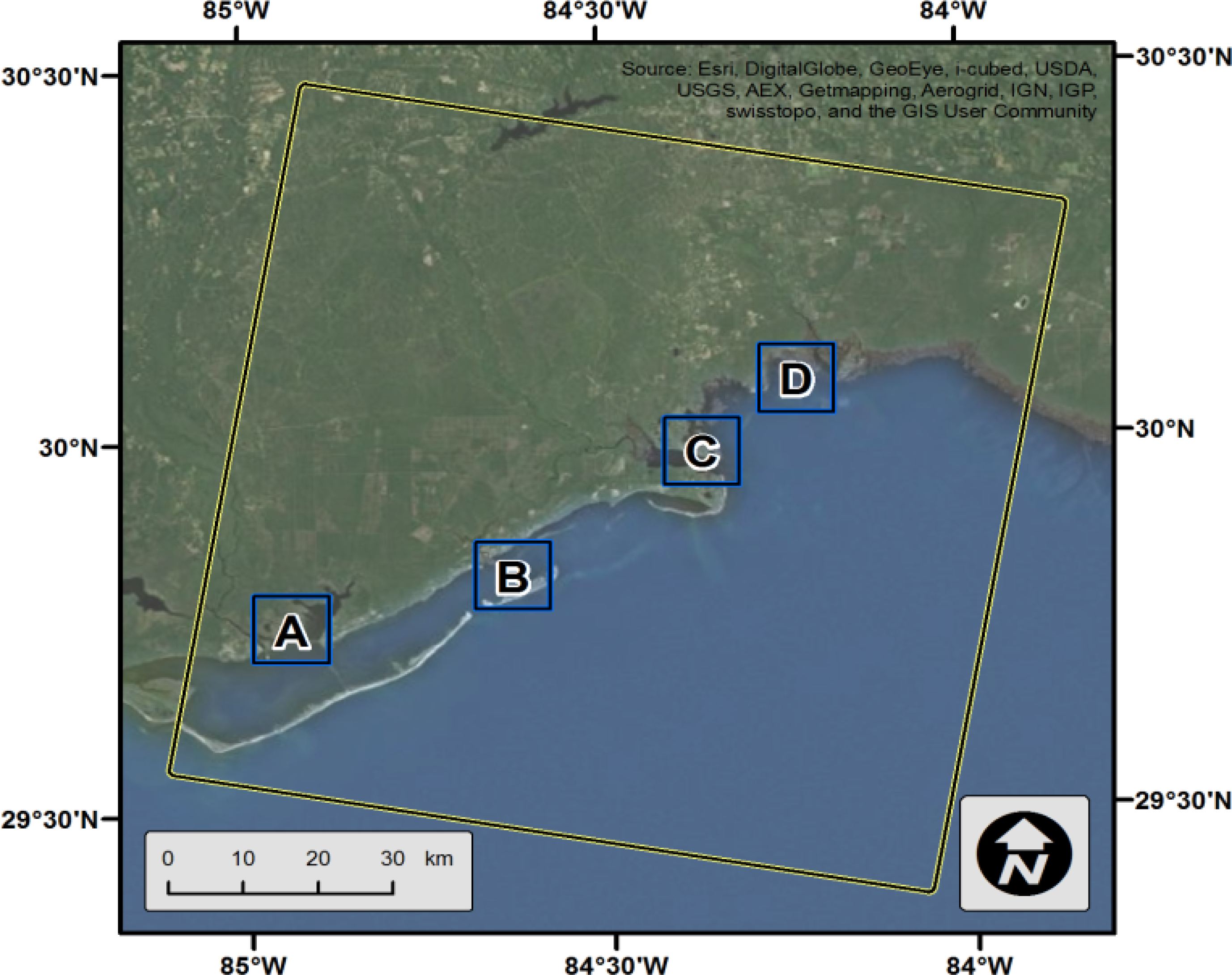
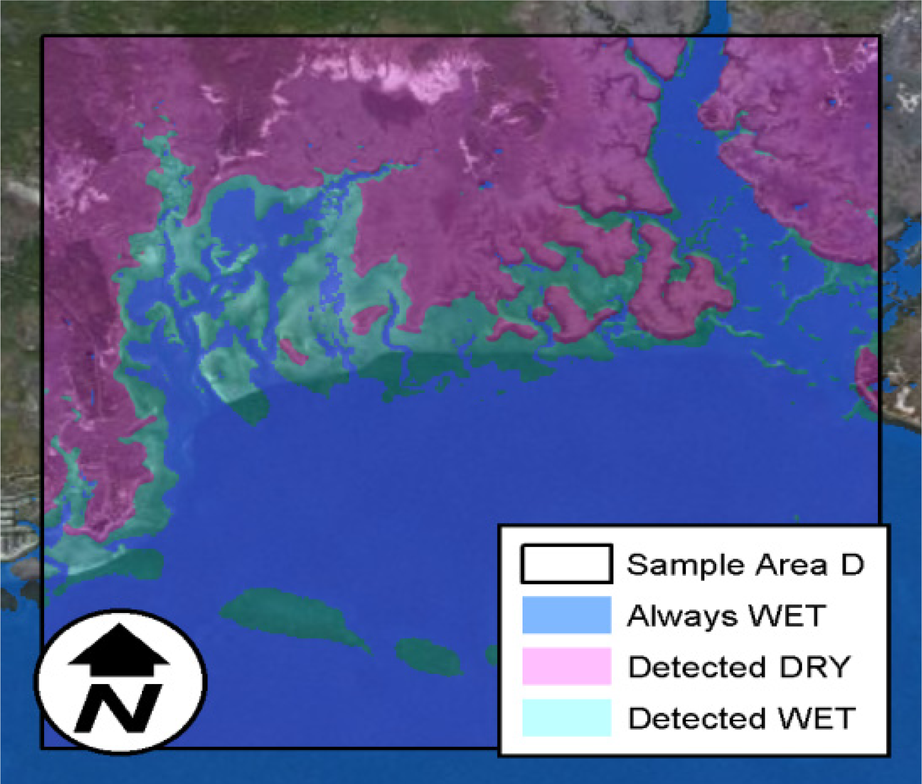
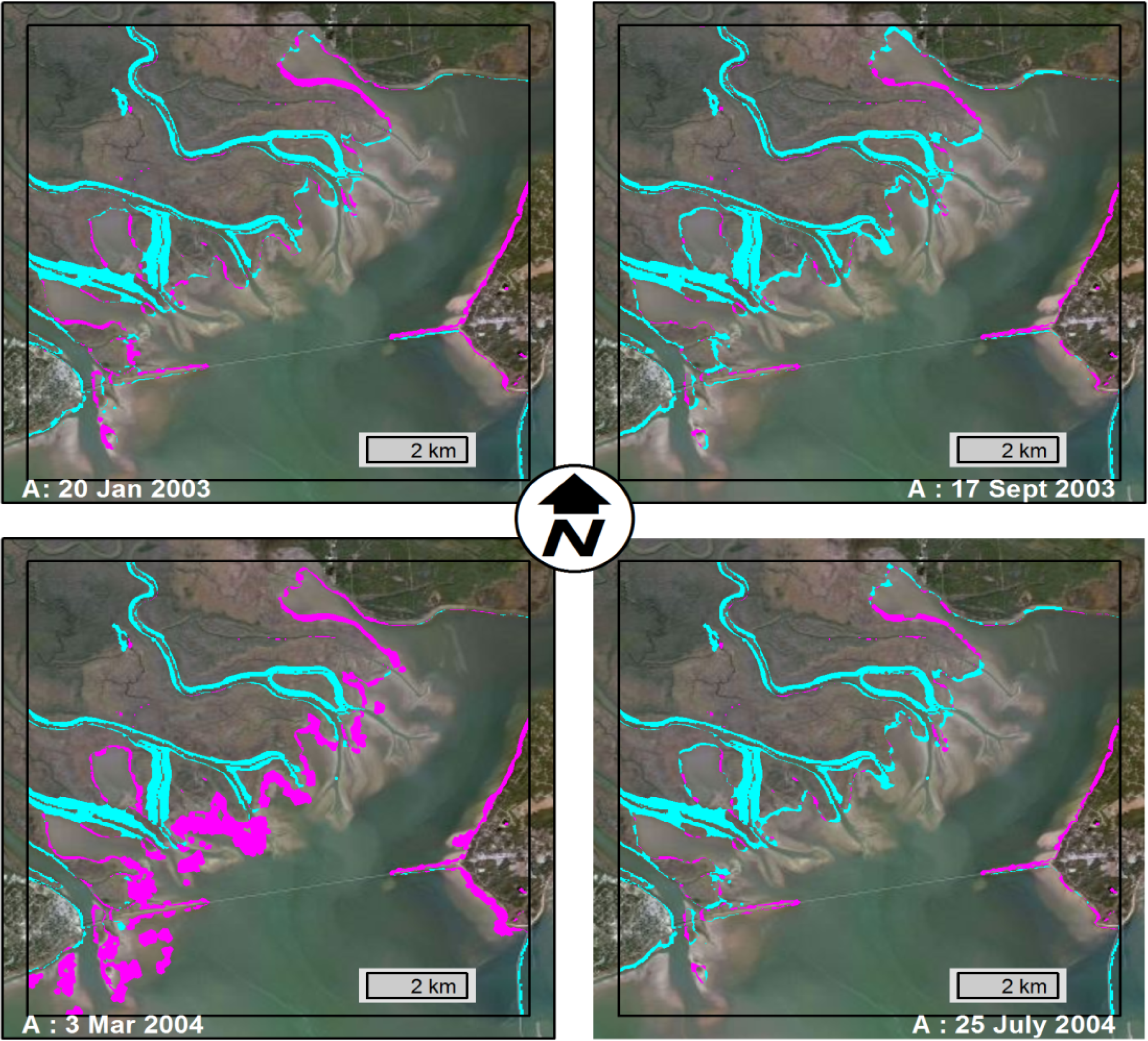
Four 10-km² areas within the boundary of one Radarsat-1 scene were selected as candidates for skill assessment. The four areas were selected because they contained extensive tidal flats and barrier islands, and also because they represent the major population and recreation centers within the study area. The assessment areas are labeled A through D running from west to east as shown in Figure 3 respectively representing Apalachicola, Carrabelle/Dog Island, Ochlockonee Bay and Apalachee Bay. 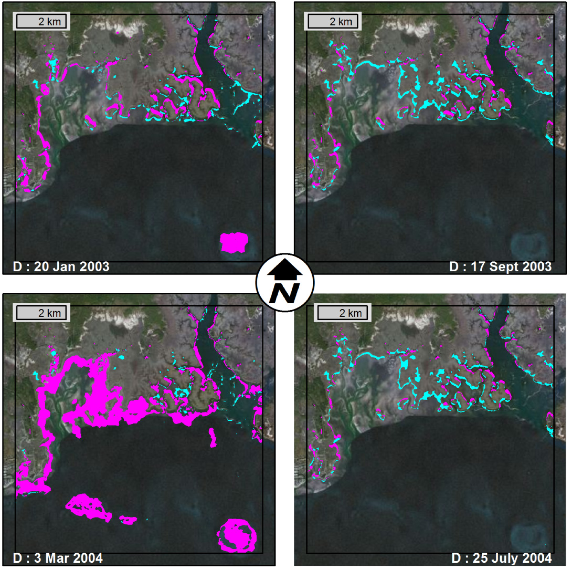An example of the raw output from the synergetic method is shown in Figure 4. Within these areas, it was necessary to convert the output from the model into a geo-referenced wet/dry image that was time synchronized with the Radarsat-1 imagery.

As stated previously, the model was simulated over four specific time periods to align with the Radarsat data and to provide a time synchronized comparison of predicted versus observed inundated area. The model produces output consisting of the elevation of the water surface at each computational point at pre-specified time intervals. In this case, the model produced output every 300 time steps or every 5 minutes for the period of time that included the specific time of the Radarsat-1 scene. The output set that corresponded to the time of the Radarsat-1 scene was extracted from the model and converted to a set of spatially distributed XYZ points with the Z value representing the water surface elevation. This set of points was converted to a one channel raster image at the same resolution of the Radarsat-1 scene where the pixels were classified as either dry or wet. The two images were then compared and model performance is assessed quantitatively using the Probability of Detection (POD) method [32,33].

The two images were compared and two POD values were computed: one for the areas that should be dry (according to the Radarsat data) and one for the areas that should be wet. POD is computed following Chaouch et al. [15]:

$$\mathit{POD}=\frac{A}{(A+C)}$$

(4)

where A = the number of pixels correctly classified as class X (either wet or dry) and C = the pixels of class X that have not been classified as class X. The hit rate, or overall classification skill of the model, is also used to measure performance. The hit rate is simply the percentage of the total number of pixels within the subarea that were classified correctly [34] and is equivalent to the average POD, weighted by the number of wet or dry pixels. Higher POD and hit rate indicate better tidal model performance. Please note that all cells within the sample areas are included in the POD calculation; no cells have been pre-classified as always wet or always dry and removed from the analysis.

4. Results and Discussion

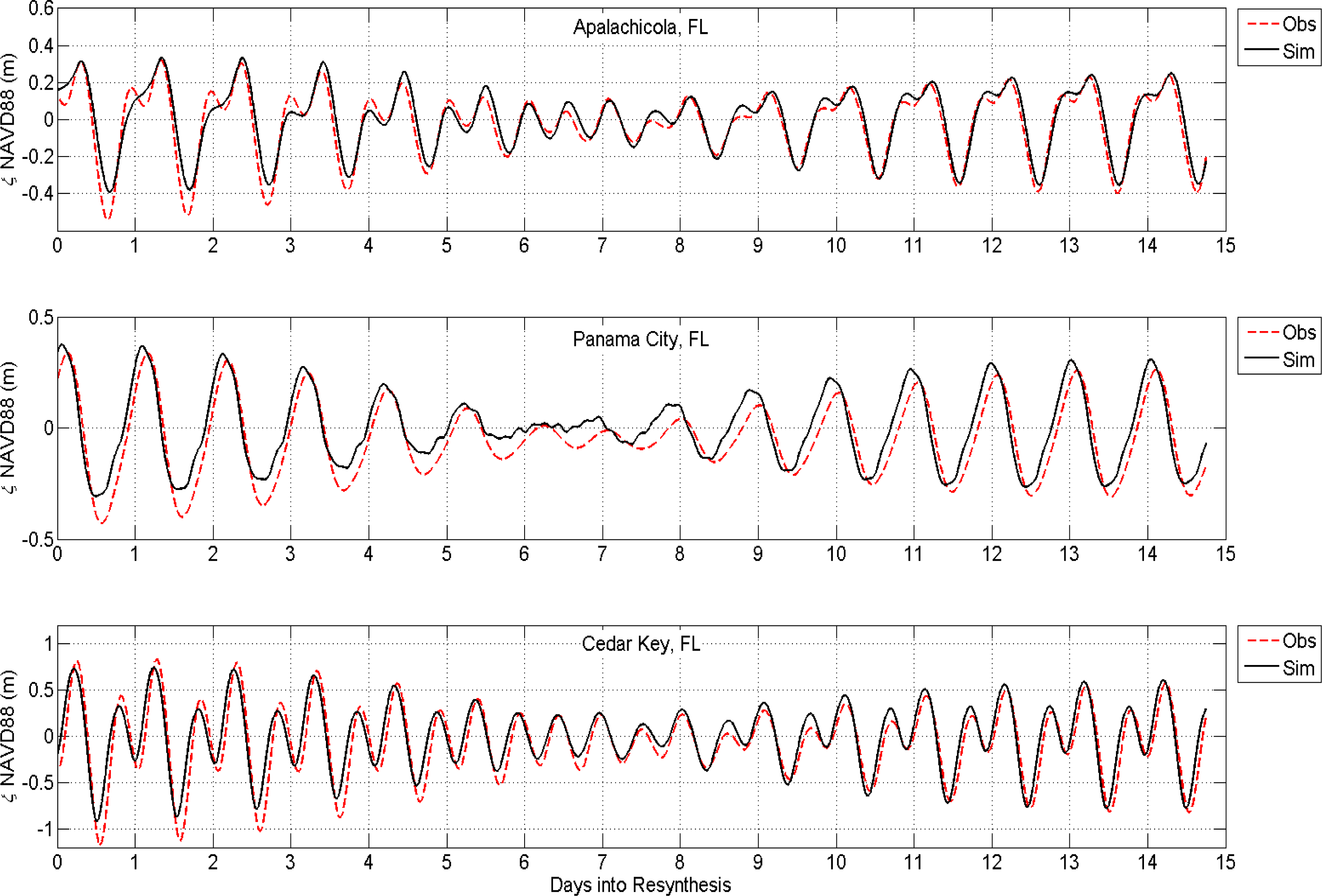
As shown in Figure 5, the model performed well when reproducing the resynthesized tides at the three NOS tide gage stations. The peaks and troughs of the tides were captured and the model appeared to be in phase. This is corroborated by the high skill and low RMSE and NRMSE results presented in

Table 3. Quantitative assessment of harmonic resynthesis results.

Station	Skill	RMSE (m)	NRMSE %
Apalachicola	0.97	0.058	6.7
Panama City	0.94	0.079	10.3
Cedar Key	0.95	0.164	8.2

. For example, at the Apalachicola station, the model produced a skill value of 0.97, a RMSE of less than 6 cm, and a NRMSE of 6.7%. The results fell within expectations as the model has 30–60 m resolution near the Apalachicola station in contrast to 4 and 4–6 km resolutions at the Panama City and Cedar Key stations, respectively. In fact, this is the primary benefit of using with models built on unstructured triangular meshes; resolution can be increased in specific areas of interest or where solution gradients are expected to be high and relaxed in areas of less concern. Therefore, the model should be more accurate at Apalachicola.

The historic water level time series comparisons for the Apalachicola station are shown in Figure 6.

Again, only the Apalachicola station lies within both the focus area and Radarsat scene boundary; therefore, NOS stations in Panama City and Cedar Key are omitted from this point on.

Assessing the performance of the model with respect to measured water level time series reveals that there are likely non-astronomic tidal physics involved such as river inflow and meteorological (wind and pressure) effects, especially during the 20 January 2003 and 3 March 2004 time periods. This is apparent in Figure 6 in the non-cyclical appearance of the observed tide around those dates (upper and lower left panels). At multiple times, such as 24 January 2003, 23 September 2003 and 6 March 2004 the observed tide displays sustained rising or falling trends that are likely caused by ambient winds. The skill measures in Table 3 and

Table 4. Quantitative assessment of synoptic simulations during the four time periods corresponding to the Radarsat scenes at the Apalachicola tide gage station.

Date	Skill	RMSE (m)	NRMSE %
20 January 2003	0.79	0.175	18.6
17 September 2003	0.83	0.138	17.7
3 March 2004	0.77	0.162	18.9
25 July 2004	0.96	0.074	8.2

corroborate this as the errors are noticeably higher on these dates.

Furthermore, in general, a model that has a high skill in terms of harmonic resynthesis and less in synoptic comparisons is usually not accounting for physics that were active during the synoptic comparisons. 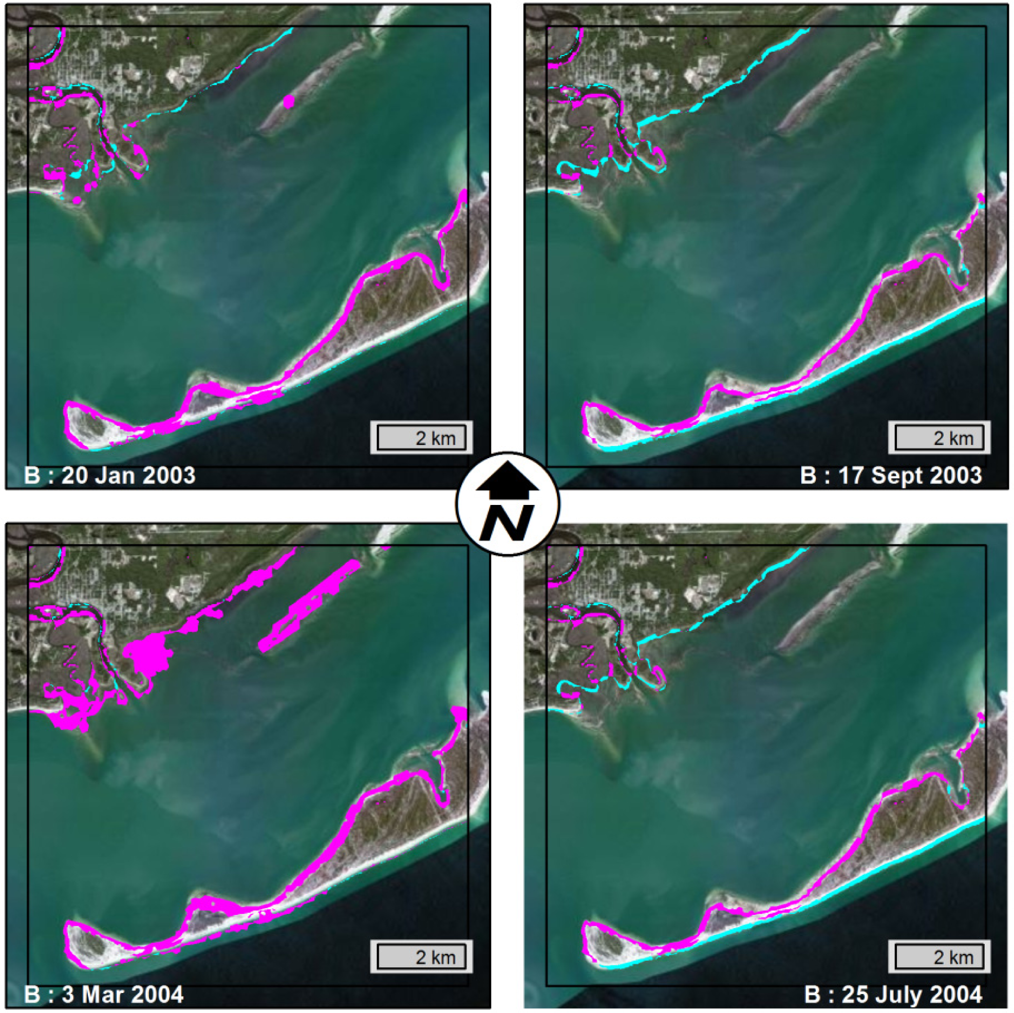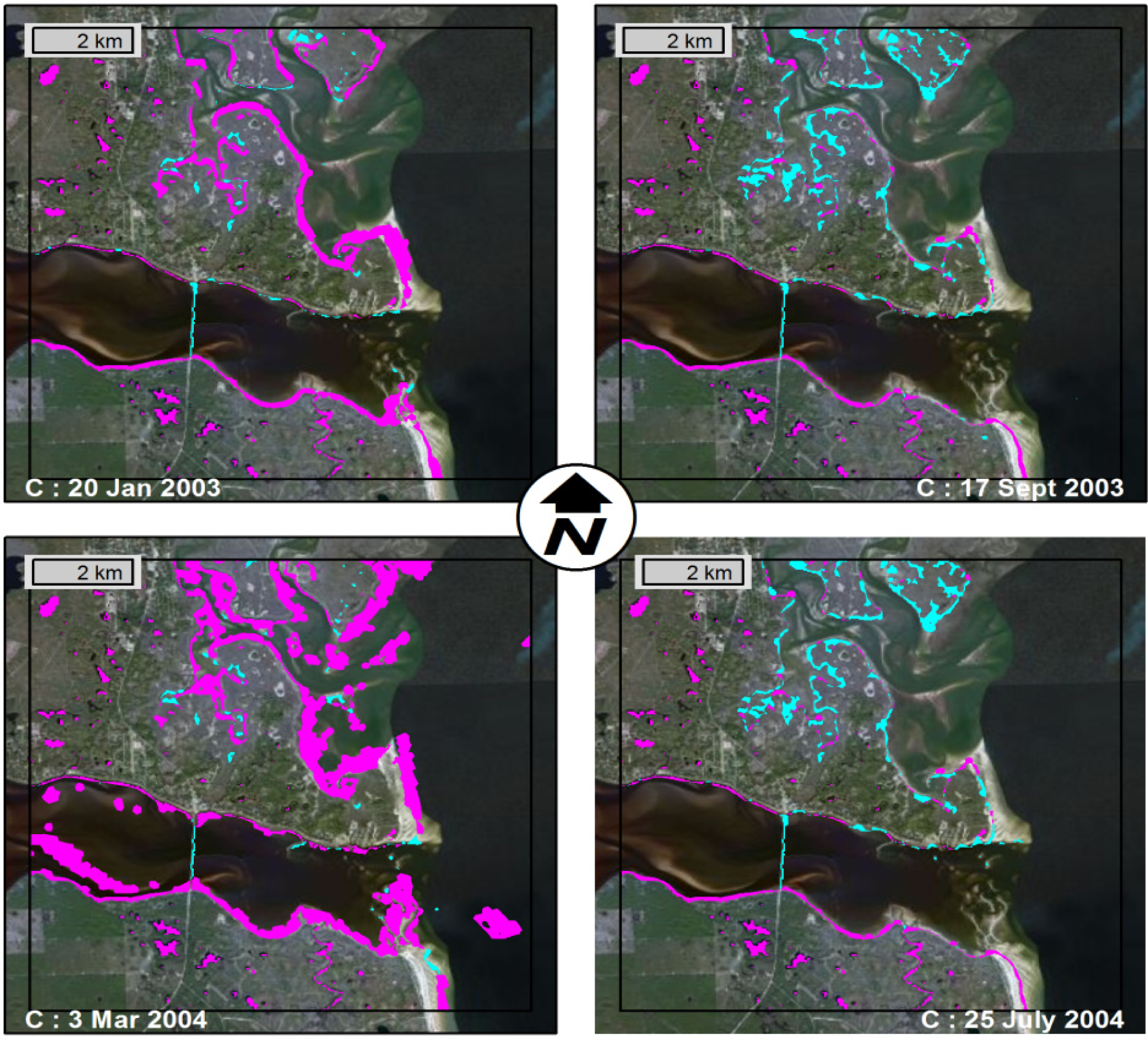The high skill in the harmonic resynthesis indicates that the model resolution, surface roughness parameterization, and topographic/bathymetric description are likely sufficient as these factors have been shown to influence tidal flooding and recession [13,35–37]. Therefore, the error in the synoptic comparisons is probably due to the absence of additional forcing mechanisms as described above. The results of the synoptic inundation area comparisons are shown in Figure 7 and Figure 10. The POD and Hit Rate values are shown in

Table 5. Probability of Detection (POD) and Hit Rate statistics for the inundated area comparison.

Area	Date	POD Wet	POD Dry	Hit Rate
A	20 January 2003	96.6%	88.8%	93.3%
	17 September 2003	98.1%	86.8%	93.3%
	3 March 2004	88.8%	90.0%	89.3%
	25 July 2004	97.8%	87.6%	93.5%
B	20 January 2003	96.1%	97.5%	96.4%
	17 September 2003	97.7%	91.1%	96.5%
	3 March 2004	92.2%	99.4%	93.6%
	25 July 2004	97.7%	92.4%	96.7%
C	20 January 2003	90.9%	99.0%	94.5%
	17 September 2003	96.3%	95.6%	96.0%
	3 March 2004	79.2%	99.0%	88.4%
	25 July 2004	96.5%	95.5%	96.1%
D	20 January 2003	94.7%	96.5%	95.3%
	17 September 2003	97.9%	93.0%	96.4%
	3 March 2004	81.8%	98.2%	87.5%
	25 July 2004	98.4%	93.4%	96.8%

.

All time periods produced hit rates greater than 85%. The model consistently performed best during the 25 July 2004 time period according to the water level time series and inundation area comparisons. This is also the time period with the least amount of non-tidal physics as indicated by Figure 6; therefore, this result is within expectations for reasons described previously. The synergetic method produced results that agreed with traditional assessment methods; simulations with weak quantitative skill values were also weaker in the synergetic method assessment.

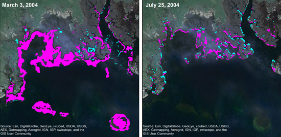
Of the four time periods studied, 3 March 2004 had the lowest water level measured at the Apalachicola station (see

Table 6. Water levels (m-NAVD88) at the Apalachicola station.

Date	Observed Water Level	Modeled Water Level	Difference
20 January 2003	−0.060	0.047	0.107
17 September 2003	0.241	0.387	0.146
3 March 2004	−0.234	−0.277	−0.043
25 July 2004	0.276	0.234	−0.042

). The majority of the error in this time period was incorrectly predicting areas as dry. One possible reason for the discrepancy in model results compared to ground truth is the issue of topographic description. Having already established that the description of the topographic/bathymetric surface is essential to an accurate model, it must be noted that the FWJ model is largely based on lidar data acquired in 2006. The FWJ model was rigorously quality checked for datum issues during development [26]; however, it is possible that the lidar data over-predicts the elevation in these salt marsh areas due to the dense emergent vegetation and water level conditions [38]. Focusing on this issue, it was immediately apparent that the synergetic method not only quantitatively assessed the performance of the model in a novel way, but it also yields information that spatially identifies potential problem areas in the model. These problem areas could be improved during model development by adding resolution and/or improving the topographic and bathymetric descriptions.

5. Conclusions

A recently developed method for detecting inundated areas based on the integration of high-resolution satellite imagery was applied to assess the performance of a tidal model of the northern Gulf of Mexico. The objective was to demonstrate the applicability of this approach and its agreement with traditional performance assessment methodologies such as harmonic resynthesis and water level time series analysis. A harmonic analysis simulation along with synoptic simulations spanning four specific historical time periods was conducted to test the performance of the tidal model.

The results indicate that the synergetic method is able to not only assess model performance in terms of quantitative skill, but also to illustrate spatial regions of model inundation error. The model was able to reproduce the extent of inundation within four sample areas inside the focus region (area of highest resolution) of the model domain and correctly identifies flooded and non-flooded areas with greater than 85% accuracy in all tests. The weakest performance occurred during time periods of significant non-astronomic tide influence. The comparisons of synoptic inundation areas generally agreed with the results of the traditional performance assessment measures and should continue to be used in concert with one another.

As the applicability of the data fusion approach has been demonstrated herein, it would benefit coastal modelers to apply it as validation protocol in conjunction with traditional methods on operational models that include all relevant forcings. However, this method is limited by the spatial and temporal (generally 1995–2008) availability of Radarsat-1 data. While Radarsat-1 provided global coverage, not all areas are available in all modes at all times. It is not freely available to the general public at this time although qualified researchers can obtain access to the data catalog through the Alaska Satellite Facility as well as a private data distribution contractor. Therefore, future work will involve adapting the technique to use other SAR sources. This method shows significant promise in advancing the development of inundation models if it can be widely implemented. This is particularly true in storm surge applications because SAR data are unaffected by cloud cover or day/night restrictions. It would be beneficial for governmental agencies to task satellites or hurricane hunter aircraft for acquiring data during tropical cyclone activity and make use of the data in real time for the monitoring of these extreme events. In conclusion, the application of the remote sensing based synergetic method will greatly benefit any endeavor where extent of inundation is modeled, predicted or hindcast.