Detection of Forest Clear-Cuts with Shuttle Radar Topography Mission (SRTM) and Tandem-X InSAR Data

Abstract

The aim of this study was to determine whether forest clear-cuts during 2000–2011 could be detected as a decrease in surface height by combining Digital Surface Models (DSMs) from the Shuttle Radar Topography Mission (SRTM) and Tandem-X, and to evaluate the performance of this method using SRTM X- and C-band data as references representing the heights before logging. The study area was located in a Norway spruce-dominated forest estate in southeastern Norway. We interpolated 11-year DSM changes into a 10 m × 10 m raster, and averaged these changes per forest stand. Based on threshold values for DSM decreases we classified the pixels and stands into the categories “clear-cut” and “not clear-cut”, and compared this to a complete record of logged stands during 2000–2011. The classification accuracy was moderate or fairly good. A correct detection was achieved for 59%–67% of the clear-cut stands. Omission errors were most common, occurring in 33%–42% of the stands. Commission errors were found in 13%–21% of the clear-cut stands. The results obtained for X-band SRTM were only marginally better than for C-band. In conclusion, the combination of SRTM and Tandem-X has the potential of providing near global data sets for the recent 12 years’ logging, which should be particularly valuable for deforestation mapping.

1. Introduction

Satellite remote sensing has a potential for increased use in monitoring forest logging [1–5]. Forest logging activities today cover large areas, which in many cases are hardly accessible for field inventories, and satellite remote sensing appears to be the only feasible approach to cover the monitoring needs. From a forest management perspective we may distinguish two needs for monitoring of logging. In tropical countries a monitoring is required within the REDD+ (Reducing Emissions from Deforestation and Degradation) framework for detection of illegal logging and for documentation of changes in forest biomass carbon stores. Deforestation and degradation has been going on at a high speed in tropical countries for decades and is a major source of carbon dioxide emissions [6]. In other countries such as Norway logging is part of a sustainable timber production, however; there are certain restrictions on clear-cutting. There are thresholds for the size of clear-cut areas, and forest owners are mandated to ensure regeneration after clear-cutting. Forest authorities need monitoring of clear-cut areas in order to check that forest owners comply with these regulations.

Several methods for remote sensing of clear-cutting exist, based on a variety of space- and air-borne sensors and methods [7–12]. For example, in Sweden clear-cut detection has been carried out with SPOT optical imagery, where new clear-cuts are detected as having an increased brightness in the short-wave infrared (SWIR) band caused by reduced shadowing [7]. A novel method is developed in Sweden based on ALOS PALSAR, where new clear-cuts are seen as having a decrease in the L-band SAR backscatter intensity [8]. High InSAR coherence has been used to detect non-forested areas and new clear-cuts [9,10] and other severe disturbances such as storm damage [13]. In tropical regions, the PRODES project in Brazil is an effort that has been going on for several years based on annual, full-coverage Landsat imagery where clear-cuts are detected from a semi-automatic pixel-unmixing classification based on soil and shadow fractions [11]. Although methods like these may work well in many cases, they have certain limitations. Applications based on optical data are limited by clouds. Particularly in some tropical forest areas there is a persistent cloud cover [14]. Another type of detection problem is a result of an increasing share of forest logging being carried out as various types of partly logging, at the expense of complete clear-cutting. In tropical countries deforestation is partly replaced by forest degradation. In countries like Norway, there is an on-going trend to increase the amount of trees left after logging. This is a result of increasing attention to bio-diversity and landscape qualities in forest management (e.g., [15,16]). The majority of trees are still logged and the logging is still considered as clear-cutting. Partly logging is less detectable with remote sensing based on spectral properties, backscatter intensity, and InSAR coherence. The remaining trees after logging have similar spectral properties as the forest before logging. Short wavelength SAR, i.e., X- and C-band, has a minor penetration into a forest canopy, and backscatter intensity and coherence may show only minor changes after partly logging.

A remote sensing approach based on 3D data, where logging detection is based on reduction in canopy height, seems feasible to overcome these limitations. A widely used 3D data type in forestry is airborne laser scanning or LiDAR. The potential and feasibility of LiDAR for disturbance monitoring has been demonstrated for detection of logging [12] and biomass changes [17], as well as storm damage [18], snow breakage [19], insect defoliation [20] and simulated forest damage [21]. In [22], the authors demonstrated the same potential and feasibility with the GLAS satellite LiDAR for storm damage. However, LiDAR methods may have some limitations related to costs and coverage as well as clouds.

Methods for clear-cutting detection based on 3D SAR may overcome the challenges related to cloud cover, data availability and coverage, as well as partly logging. Recently, two Digital Surface Models (DSMs) were generated by 3D SAR methods, and it was demonstrated how decreases of at least 8–10 m in the DSM corresponded to forest degradation in tropical forests [23]. They subtracted an SRTM DSM from a DSM generated by Cosmo Skymed spotlight data. With short wavelength SAR, i.e., X- and C-band, the RADAR echo is located high up in the forest canopy [24], and height changes should be a sensitive indicator for disturbance. Forest height and related variables such as stem volume and biomass have been correlated to 3D SAR height, i.e., both interferometric height [25–32] and radargrammetry height [33–35].

In the present study we present another 3D SAR approach, which in line with [19] might overcome the limitations with existing methods, and in addition has a potential to provide near-global data. We use Tandem-X data in combination with SRTM. The Tandem-X mission will provide a global DSM. If disturbance detection turns out to be feasible with a combination of SRTM and Tandem-X, that would enable detection of clear-cuts and disturbances at large and near-global scale. In the REDD+ framework this could be particularly valuable by providing a 10–12 year logging record, which might serve as business-as-usual baseline data [14]. However, there are some possible challenges with this approach. Rather than using SAR data in spotlight mode as [23], we apply the standard stripmap mode of Tandem-X. Stripmap data has a higher areal capacity than spotlight; however, this comes at the expense of spatial resolution, and this may reduce the performance for logging detection. Another challenge is the difference in wavelength between the C-band in SRTM and the X-band in Tandem-X. A 3 m height difference between the C- and X-band SRTM DSMs in a Norwegian forest was found by [32]. In [23], the authors demonstrated that this may not be a problem. However, we had a unique data set for quantifying the effect of this problem, and for testing the method in general. Our study area is located in southern Norway, where both the X- and the C-band SRTM DSMs were available with full areal coverage.

The objectives of this study were:

(1)

to determine whether clear-cut areas during 2000–2011 could be detected as a decrease in DSM height from SRTM to Tandem-X, and

(2)

to evaluate the performance of this method using SRTM X- and C-band data as references representing the heights before logging.

2. Materials and Methods

2.1. Study Area

The study was carried out in a 98 km² part of a private forest estate in the municipality of Lardal in southeast Norway. The center of the study area was at 59.36° north and 9.87° east. The study area was covered by a forest management plan which included delineation into 3,181 forest stands. A forest stand database contained the outline of each stand, in which each stand had a unique stand number. This was supplemented by logging records in the form of a table, where each logging was one record. Each record contained stand number, date and logging category. We extracted logging records during the 11 year period from the SRTM acquisition to the Tandem-X acquisition, using the starting date 20 February 2000 and ending date 23 July 2011. The categories included mainly clear-cut and thinning, but also a few other logging types which we grouped as “miscellaneous”. A few stands had repeated loggings with different logging categories, and we assigned the most severe of these categories to those stands. The stands were now distributed with 260 stands (8.2%) on clear-cut; 373 (11.7%) on thinning; 40 (1.3%) on miscellaneous, while 2,508 (78.8%) stands had no logging during the 11 years. In this way we had logging records present at the stand level, i.e., as an attribute of the entire stand. We converted this to a 10 m × 10 m raster, by which all cells within the stand outline were assigned the same logging category as the stand. From an airborne laser scan of the study area with a pulse density of 10 m⁻², we generated a Digital terrain Model (DTM), which were used for visualization of the results. Throughout the study we worked both at the stand level and at the pixel level.

2.2. InSAR DSMs

Logging was to be detected as a decrease in canopy height. We derived 11 years temporal differences from SRTM to Tandem-X, and focused on negative height changes. We used both the X- and C-band InSAR DSMs from SRTM, which was carried out during 12–20 February 2000 [36]. Both the X- and C-band DSMs have full areal coverage in the study area, i.e., up to 60° north in southern Norway. SRTM acquired bi-static data by mounting SAR sensors both in the shuttle body and on the tip of a 60 m extended boom. The X-band data were acquired with a stripmap system, while The C-band data were acquired with a scanSAR system of the Spaceborne Imaging Radar-C (SIR-C) hardware. We received the X-band InSAR DSM from the German Aerospace Centre (DLR) in 2002. The data were received in geographic (lat/lon) projection with a spatial resolution of 1 arc sec which at our study area corresponded to approximately 15 m × 31 m. The C-band InSAR DSM data was derived from a procedure built into the ENVI/Sarscape 5.0 software, which downloads data as SRTM-3 version 4 [37]. The spatial resolution of 3 arc sec corresponded to approximately 46 m × 93 m. We carried out a bilinear resampling to UTM32 and to a common spatial resolution of 10 m × 10 m used for both DSMs.

We utilized an ascending, right looking TanDEM-X stripmap image pair acquired in the afternoon (16:54) on 23 July 2011. The polarization was HH and the incidence angle was 36°. During 24 h around the acquisition the mean temperature was 15 °C and the weather was rainy with 40 mm precipitation. The data were received from DLR as co-registered Single Look Complex (SLC) data in CoSSC format. The InSAR processing was carried out with the ENVI/Sarscape software, separately with the X- and C-band SRTM DSMs as references. For each of them the following processing was carried out: An interferogram was generated, and this was processed into a differential interferogram by using the SRTM DSM as reference file. The differential interferogram represented mainly the phase differences caused by 11 year changes in vegetation height. The differential interferogram had a dominating phase value, i.e., a certain phase value that covered the majority of the study area where none or minor height changes had occurred. In addition, there were scattered areas of other phase values clearly caused by logging or other changes in vegetation height, as well as scattered pixels with phase noise. Lakes and rivers were particularly noisy due to low backscatter and low coherence. We applied the Goldstein filter [38] to reduce phase noise, and thereby enabling an accurate phase unwrapping. In addition, the differential interferogram also contained possible errors originating from inaccuracies in the SRTM DSMs, inaccuracies in the Tandem-X orbit data, and atmospheric effects. Such possible errors would mainly lead to a vertical offset or a ramp error, and in order to remove such errors we fitted Equation (1) to 25 Ground Control Points (GCPs) distributed over the study area. The GCPs were placed roughly in a systematic 5 × 5 manner over the image; however, they were subjectively and carefully placed where there was no apparent 11 year change, i.e., where the filtered, differential interferogram had a phase value close to the dominating value, and where the fringe density was low. Noisy areas such as lakes and rivers where avoided.

$$\Delta \varphi =k_0+k_1\text{RG}+k_2\text{AZ}$$

(1)

Δϕ was the phase difference at each GCP, k₀, k₁ and k₂ were correction factors, and RG and AZ were the range and azimuth co-ordinates (

Table 1. Correction factors for phase offset and phase ramp errors (radians), see Equation (1), and the final accuracy (RMSE) for the 25 Ground Control Points (GCP).

Reference DSM	k0	k1	k2	RMSE
SRTM-X	−0.1130	2,069 × 10−7	−523 × 10−7	1.1 m
SRTM-C	0.1393	457 × 10−7	264 × 10−7	1.5 m

). After correcting the differential interferogram with these factors the RMSE of the GCP heights were 1.1 and 1.5 m, respectively for the X- and C-band DSMs.

The normal baseline was 122 m and the corresponding 2π height of ambiguity was 23 m. This is less than the possible range of DSM changes from 2000 to 2011. Hence, the differential interferogram could not be directly recalculated to vegetation height changes, and we carried out phase unwrapping using the Minimum Cost Flow method. The unwrapped phases were converted into elevation data and transformed from satellite slant-range geometry to a geocoded DSM. We checked for unwrapping errors. There were layover or shadow problems in 88 stands. All these stands had layover or shadow problems from the InSAR processing with the X-band SRTM as reference, while only 4 of them had such problems with the C-band SRTM. On average 11% of the area of these 88 stands were affected. In order to check the sensitivity of our results for such problems, we initially carried out a few of the analyses both for the entire data set and after excluding these 88 stands. The exclusion of these stands had no or minor influence on the results. The classification accuracy at the stand level increased from 95.5% to 95.7% with the X-band SRTM, and it remained unchanged for the C-band SRTM. Hence, we retained all stands in the data set for analyses. We also checked the DSMs for other possible discontinuities. A few scattered occurrences of very steep slopes up to 67° in the DSMs turned out to be real steepness at forest edges and steep hillsides. During the processing we used a multi-looking of 5 azimuth × 6 range, which corresponded to about 10 m × 10 m, which was also the spatial resolution of the geocoded DSMs obtained by cubic convolution resampling. By subtracting each of the SRTM DSM’s from the Tandem-X DSM we obtained two datasets representing 11-year changes in surface height. We calculated the mean DSM change for each of the 3,181 forest stands based on the pixel values.

2.3. Analysis for Detection of Clear-Cuts

Based on the DSM changes we classified the study area into two categories; “clear-cut” and “not clear-cut”. We used a heuristic approach, with a threshold value to separate the two classes. We tried a range of threshold values and iteratively identified the threshold that minimized the sum of omission and commission errors:

$${\mathit{Omission}}_{\mathit{error}}=\sum x_o/N$$

(2)

$${\mathit{Commission}}_{\mathrm{error}}=\sum x_c/N$$

(3)

where x_o is a clear-cut pixel or stand which is misclassified as not clear-cut, x_c is a not clear-cut pixel or stand which is misclassified as clear-cut, and N is the number of pixels or stands with clear-cut. We did this separately with the X- and C-band SRTM data, and separately at the pixel and the stand level.

3. Results

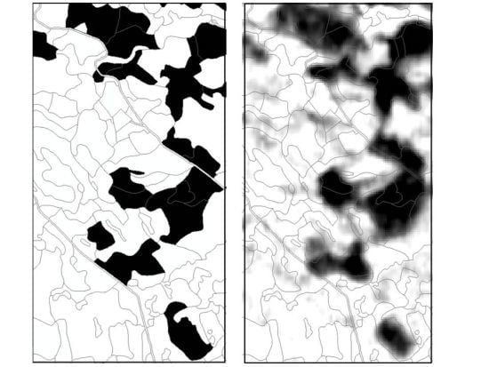
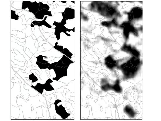
The 11-year change in DSM height from SRTM to Tandem-X was a moderate, or fairly good, predictor of occurrence of clear-cuts, although errors occurred quite frequently. The results were only marginally better with the X-band than with the C-band SRTM DSM as reference. The results obtained for the entire study area corresponded well to what is visible in Figures 1 and 2. The DSM decreases seen at the pixel level (Figure 1, right panel) corresponded well to the recorded clear-cut stands (Figure 1, left panel). The stands had characteristic and rugged outlines, which is typical for Norway’s forests where topography and edaphic factors vary considerably over short distances. Clearly, the DSM decreases at the pixel level followed these characteristic stand outlines. However, some discrepancies were also evident. Some jaggy details of the stand outlines were not seen at the pixel level. In some cases a part of a stand appears to not have been logged, and in other cases the logged area appears to be larger than the stand. It is likely that the clear-cuts have not entirely followed the stand borders present in the forest management plan and that this caused part of the observed discrepancies. 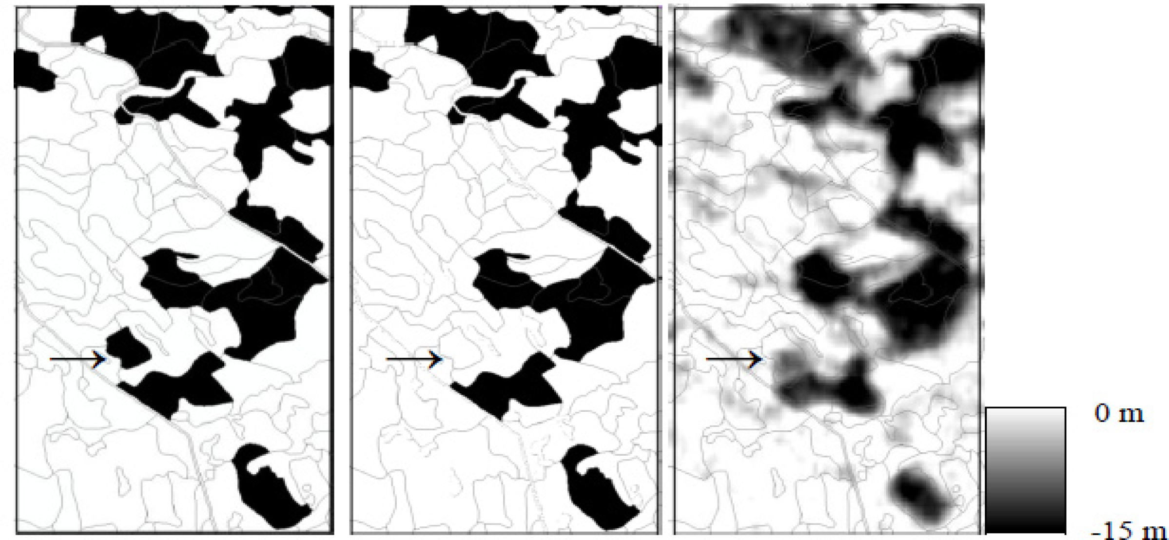Close to the center of Figure 1, center panel, there is a small, misclassified clear-cut stand. A closer look at the pixel level changes revealed clear DSM decreases only in the southern half of that stand. The stand is indicated with an arrow in Figures 1 and 2.

With C-band SRTM the result was noisier at the pixel level, although a considerable amount of details were still picked up (Figure 2, right panel). There was still a fairly good correspondence with the logging records at the stand level. Figure 2 shows some classification errors. Two of the clear-cut stands visible here were misclassified as not clear-cut, while two stands without clear-cut were misclassified as clear-cut.

For the entire study area the classification accuracy obtained with the X-band SRTM was only slightly better than that obtained with C-band. At the stand level, the best result was obtained with a threshold of −7 m for X-band (

Table 2. Results with X-band SRTM at the stand level: Confusion matrix (%) of stand classification against the logging records. The classification threshold was −7 m DSM change (N = 3,181 stands).

		Reference		User’s Accuracy
		Clear-Cut	Not Clear-Cut
Classified	Clear-cut	5.4	1.7	76.1
	Not clear-cut	2.7	90.1	97.1
	Produser’s accuracy	66.7	98.1	Overall accuracy 95.5

). This was the threshold where the sum of omission errors and commission errors was at minimum. Omission errors were the most common error. Clear-cuts were recorded in 8.2% of the stands. Out of these 8.2% there was a mis-classification as not clear-cut in 2.7%, which means an omission error of 33%. This corresponded to a 67% producer’s accuracy for clear-cut detection. The commission error (false detection of clear-cut stands) was 21%, corresponding to a 76% user’s accuracy for detection of not clear-cut stands. The overall accuracy was 96%; however, this very high number is largely obtained because 92% of the stands had not been clear-cut.

For C-band SRTM, the best stand-level classification result was obtained by applying a threshold of −9 m. In comparison with X-band the omission error was higher (42%) while the commission error was lower (13%). These numbers corresponded to a 59% producer’s accuracy for clear-cut detection and an 81% user’s accuracy for non-clear cut detection. Again the overall accuracy was 96% (

Table 3. Results with C-band SRTM at the stand level: Confusion matrix (%) of stand classification against the logging records. The classification threshold was −9 m DSM change (N = 3,181 stands).

		Reference		User’s Accuracy
		Clear-Cut	Not Clear-Cut
Classified	Clear-cut	4.8	1.1	81.4
	Not clear-cut	3.4	90.8	96.4
	Produser’s accuracy	58.5	98.8	Overall accuracy 95.6

).

At the pixel level (N = 982,533) the thresholds were slightly different and the accuracies were somewhat lower than at the stand level. Again the accuracies obtained with X- and C-band SRTM data were similar. The best threshold for pixel classification with X-band SRTM was a DSM change of −10 m, which resulted in an omission error of 48% and a commission error of 17%. With C-band SRTM the best threshold was −11 m, which produced an omission error of 51% and a commission error of 17%.

Other types of logging were less easily detected. While the mean DSM change in clear-cut stands was a 9–10 m decrease, stands without clear cutting or with another logging type had mostly small decreases or increases (

Table 4. Statistics for change in DSM distributed on logging categories (N = 3,181 stands).

Logging Category	From SRTM X Mean (min/max)	From SRTM C Mean (min/max)	Area%
None	0.6 (−16.3/31.9)	−0.6 (−16.5/20.8)	78.8
Thinning	1.0 (−8.1/12.3)	−0.8 (−11.6/12.7)	11.7
Miscellaneous	−3.9 (−14.4/2.6)	−4.3 (−16.3/4.3)	1.3
Clear-cut	−9.0 (−20.4/4.2)	−9.7 (−20.8/10.7)	8.2

). Thinning was the most frequent type of logging (11.2% of the stands). Thinned stands could not be distinguished from stands without logging as seen from DSM changes. The mean change was close to zero for thinned stands, as was the case for the stands with no logging. Miscellaneous loggings had a more pronounced decrease (approximately 4 m), but not as strong as for clear-cuts. There were considerable ranges in DSM change for all the logging categories with large overlaps between them.

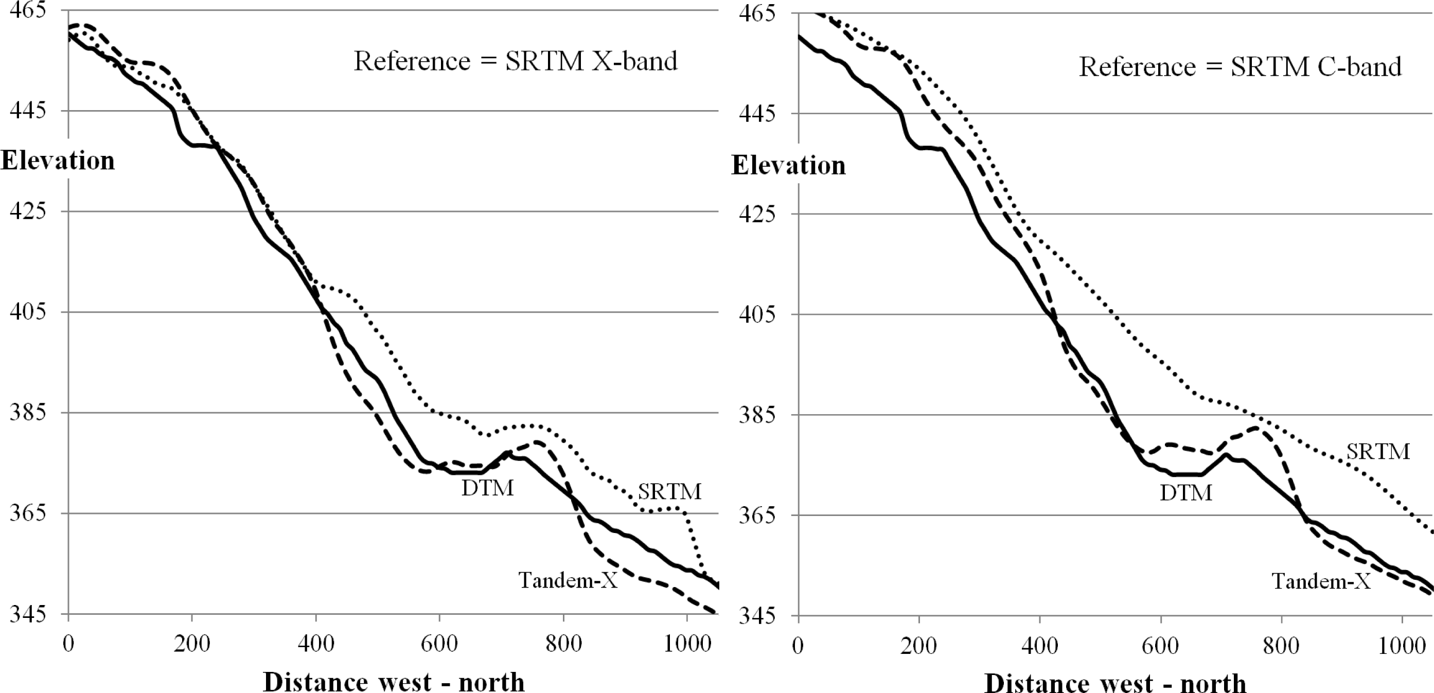
The SRTM X-band DSM had a negative bias of about 5 m; however, this had no influence on the clear-cut detection. On average this DSM had 5.2 m lower values than the SRTM C-band DSM over the study area. This resulted in the Tandem-X DSM generated with the SRTM X-band DSM as a reference to have lower values than the one generated with the SRTM C-band DSM as reference, on average 4.9 m lower. This is exemplified for a 1 km transect (Figure 3). The X-band SRTM DSM was close to the ground in the left part of the transect, while the C-band SRTM DEM indicated a tall forest here. The Tandem-X DSM generated with the X-band as reference had often below ground values. However, the temporal change in elevation from SRTM to Tandem-X is very similar for X- and C-band SRTM. With the present InSAR processing method the Tandem-X DSM was forced down on the SRTM-DSM, by using GCPs in non-vegetated locations. Apart from this, Figure 3 shows that the X-band SRTM DSM contained more details than the C-band SRTM DSM, which is as expected due to its higher spatial resolution.

4. Discussion

The first objective of this study was to determine whether a combination of SRTM and Tandem-X DSMs could be used to detect clear-cut activity during an 11-year period. The results showed that this method had a moderate or fairly good ability to detect clear-cuts carried out during the 11 year period in this study area. There were a significant number of classification errors totaling 55% of the total number of clear-cut stands. However, we consider this to be a reasonably good result given the study area and the length of the investigated time period. The main point here is that the present forest has been actively managed for decades, and contained a patchy mosaic of stands of different ages and heights during the entire 11 year study period. While the recent Tandem-X data set had the ability to pick up these variations in forest height over small distances, this ability was lower for the smooth and low-resolution SRTM DSMs.

The present method works even when there are large scale errors on the SRTM DSMs, such as vertical offsets or ramps. This is an important advantage for applying this method operationally. There is no need to correct vertical offset or ramp errors in the SRTM DSM prior to the analyses. The produced InSAR DSM can be forced down on the SRTM DSM by laying out GCPs in locations with none or minor height changes, e.g., agricultural fields. The resulting height changes over time will in this way be unaffected by such errors.

During a period of 11 years there are several reasons for significant changes in both actual canopy height and in observed DSM. Being a forest managed for timber production the clear-cuts are quickly regenerated and the young stands may grow a few meters in height during an 11-year period. Other logging activities than clear-cutting were carried out in 13% of the stands. Hence, in this study the not clear-cut category of stands contained a number of thinning and other types of logging that have reduced the canopy height, and some of these stands might have been confused with clear-cuts. Furthermore, as mentioned in the introduction, today’s clear-cuts contain some old trees that are left standing due to biodiversity and landscape considerations. Thus, the clear-cuts become less distinguishable from the not harvested stands especially at the pixel level, where the canopy may actually not have been strongly influenced by the clear cut.

Some errors in clear-cut detection could be related to SAR acquisition and geometry. In our study area it is likely that the SRTM had a dominance of north-facing acquisitions, because the Endevour space shuttle was here at its northern peak of the orbit. The Tandem-X acquisition, in comparison, was east-facing. This difference in look direction will generate some DSM differences in a hilly terrain such as present in our study area. Coming at a slant angle, the SAR microwave pulses will penetrate deeper down into vegetation in hillsides facing towards the sensor than in hillsides facing away from the sensor. Secondly, the SRTM had a coarser spatial resolution than the Tandem-X and had to be resampled prior to this study. This will lead to some errors in DSM changes. Finally, the SRTM and Tandem-X data were acquired during winter and summer, respectively. The penetration into the vegetation may have been deeper during the SRTM winter conditions, as the dielectric constant decreases when the vegetation freezes [39]. Hence, it is likely that if a monitoring system for clear-cuts was established with SAR acquisitions having the same geometry and repeated in the same season, the accuracy would have been higher than what was obtained in the present study.

Another source of error in this study is inaccuracies in the logging records. This means that the potential accuracy of the method is somewhat higher than what was found in this study. The logging category of the stand was assigned to all the 10 m × 10 m pixels within the stand. It was evident that the logging did not always follow the stand outline present in the forest management plan. This was a result of inaccuracies in the stand outline, i.e., the stand outline present in the database was not completely consistent with the applied outline in the field. In addition, sometimes the foresters have harvested only one part of a stand. This explains errors both at the pixel and stand level. At the pixel level, there are mainly pixels along the stand outline that were affected by this error. At the stand level, there were mainly stands that were only partially logged that were prone to misclassifications. The harvesters’ have largely used GPS tracking, and the tracking logs might have provided more accurate logging records.

The second objective of this study was to quantify the difference in the performance with X- and C-band SRTM as reference data. Surprisingly, the overall classification performance was similar. Visual inspection (Figures 1 and 2) indicated that the DSM changes based on the X-band SRTM contained more details and less errors than those based on the C-band SRTM. However, the sum of omission and commission errors was almost identical for X- and C-band SRTM, both at the stand-level and at the pixel-level. This may seem surprising, as the X-band DSM was based on the same wavelength as the Tandem-X, and in addition it had a spatial resolution that was 3 times higher than the C-band DSM. We believe that the explanation for this is that the present change detection relies mainly on the high level of details in the Tandem-X DSM, while both SRTM DSMs are fairly crude references. This corresponds to the “SRTM Difference Approach” of [23], who detected forest disturbance in Cameroon and the Republic of Congo by combining the SRTM C-band DSM and a Cosmo Skymed spotlight radargrammetry DSM. In their study the C-band SRTM DSM was very smooth, and the temporal changes were largely resulting from the details in the Cosmo Skymed DSM. [23] used a somewhat similar 3D SAR approach as in the present study, by combining SRTM and a 3D SAR DSM from radargrammetry processing of a Cosmo Skymed spotlight image pair. They used height change threshold values of 8–10 m for logging detection, which is similar to the present study. We obtained somewhat larger errors in clear-cut detection than [23]. While our omission errors were 33%–42%, they had errors in the range 16%–21%. Our commission errors varied between 13% and 21%, while they had 6%–13%. There are two likely explanations for the better performance in the study of [23]. First, the spotlight data has a higher spatial resolution than the stripmap data. Secondly, degradation in a tropical forest is normally a change from a virgin forest to a disturbed forest, and it typically occurs over a larger area than the average clear-cut size of 1.8 ha in our study area. The canopy layer changes from a smooth surface in a virgin rainforest to a rugged surface, and the use of a coarse SRTM DSM at the first point of time and a high resolution spotlight DSM at the second point of time fit well with this change. In our study area the forest has been actively managed at the stand level for many decades, and the SRTM DSMs have a limited ability to represent the ruggedness of the forest surface in the year 2000. Hence, it is likely that we would have obtained a higher accuracy in a forest that changed from a virgin forest with a smooth canopy height over large areas in 2000, e.g., in a virgin tropical forest.

To some extent we can compare our approach with other methods, although different methods are not always directly comparable and the difference in the study areas characteristics has a large influence on the results. We classified about 50% of all pixels within clear-cuts correctly, which is lower than the 60% [8] obtained with repeated PALSAR data. However, they used repeated acquisitions with only 1 year difference, and taken from the same orbit position. We had 33%–42% omission errors and 13%–21% commission errors at the stand level, while [8] had omission errors in the range 19%–75% and commission errors in the range 0%–21% for detection of snow damage in single trees with airborne LiDAR. We had an overall classification accuracy of 96% for clear-cut versus no clear-cut at the stand level, while [21] obtained 88% for disturbance mapping with airborne LiDAR.

The present study, as well as the study by [23], is promising for two types of applications. First, detecting clear-cuts as a decrease in 3D SAR DSMs may become a useful method in countries like Norway, where more trees are left in today’s clear-cuts. The method should also be useful for detection of other major disturbances such as wind-throw. Secondly, the method has a potential in monitoring tropical forests as part of the REDD+ initiative. Possibly, the combination of SRTM and a recent 3D SAR DSM might be used for determining the business-as-usual baseline for the recent decade’s forest logging activities. The availability of a global Tandem-X DSM, as well as the SRTM DSM, may enable a large-scale, or near-global, application of 3D SAR approaches for 11-year logging detection.

Further research is needed to test the method in tropical forests as part of the REDD+ initiative. Additionally, the use of 3D SAR for detection of loggings may potentially be refined to include estimation of the associated losses in biomass and carbon. It has been shown that above-ground biomass has a strong and linear correlation to InSAR height, (i.e., the height above ground of the center of the backscatter) [29–31]. Hence, it might be possible to also estimate the biomass loss due to a DSM decrease in a detected clear-cut. There is also a need for testing the need for correction factors for effects of weather conditions and topography.

5. Conclusions

Clear-cut stands were identified as having a DSM decrease of 7–10 m, which resulted in a correct detection of 59%–67% of the clear-cut stands and an overall classification accuracy for clear-cut versus not clear-cut stands of 95%. The combination of C-band SRTM and X-band Tandem-X has the potential of providing near global data sets for the recent 12 years of logging. The difference in wavelength appears to have negligible influence. Due to the coarser spatial resolution of the SRTM the method should be particularly useful for forests which had a smooth and even canopy height in 2000 and a variable canopy height due to loggings now. Hence, it should be suitable for deforestation mapping within REDD, as a supplement to carbon stock monitoring.

References

1. Kuntz, S. Potential of spaceborne SAR for monitoring the tropical environments. Trop. Ecol 2010, 51, 3–10. [Google Scholar]
2. Lynch, J.; Maslin, M.; Balzter, H.; Sweeting, M. Choose satellites to monitor deforestation. Nature 2013, 496, 293–294. [Google Scholar]
3. Patenaude, G.; Milne, R.; Dawson, T.P. Synthesis of remote sensing approaches for forest carbon estimation: Reporting to the Kyoto Protocol. Environ. Sci. Policy 2005, 8, 161–178. [Google Scholar]
4. Frolking, S.; Palace, M.W.; Clark, D.B.; Chambers, J.Q.; Shugart, H.H.; Hurtt, G.C. Forest disturbance and recovery: A general review in the context of spaceborne remote sensing of impacts on aboveground biomass and canopy structure. J. Geophys. Res.: Biogeosci. 2009, 114. [Google Scholar] [CrossRef]
5. Kuntz, S.; von Poncet, F.; Baldauf, T.; Plugge, D.; Kenter, B.; Köhl, M. A Multi-Stage Inventory Scheme for REDD Inventories in Tropical Countries. Proceedings of the 34th ISRSE Conference, Sydney, NSW, Australia, 10–15 April 2011.
6. Global Forest Resources Assessments. 2005. Available online: http://www.fao.org/docrep/008/a0400e/a0400e00.htm (accessed on 1 July 2013).
7. Willén, E.; Rosengren, M. Satellitdata för Skoglig Planering; Metria: Stockholm, Sweden, 2003. [Google Scholar]
8. Santoro, M.; Pantze, A.; Fransson, J.E.S.; Dahlgren, J.; Persson, A. Nation-wide clear-cut mapping in sweden using ALOS PALSAR strip images. Remote Sens 2012, 4, 1693–1715. [Google Scholar]
9. Askne, J.I.H.; Dammert, P.B.G.; Ulander, L.M.H.; Smith, G. C-band repeat-pass interferometric SAR observations of the forest. IEEE Trans. Geosci. Remote Sens 1997, 35, 25–35. [Google Scholar]
10. Solberg, S.; Astrup, R.; Lyytikainen-Saarenmaa, P.; Kantola, T.; Holopainen, M.; Weydahl, D.J.; Kaartinen, H. Testing TerraSAR-X for Forest Disturbance Mapping. Proceedings of the 4th TerraSAR-X Science Team Meeting, Oberpfaffenhofen, Germany, 14–16 February 2011.
11. Hansen, M.C.; Shimabukuro, Y.E.; Potapov, P.; Pittman, K. Comparing annual MODIS and PRODES forest cover change data for advancing monitoring of Brazilian forest cover. Remote Sens. Environ 2008, 112, 3784–3793. [Google Scholar]
12. Yu, X.W.; Hyyppa, J.; Kaartinen, H.; Maltamo, M. Automatic detection of harvested trees and determination of forest growth using airborne laser scanning. Remote Sens. Environ 2004, 90, 451–462. [Google Scholar]
13. Dwyer, E.; Pasquali, P.; Holecz, F.; Arino, O. Mapping forest damage caused by the 1999 Lothar Storm in Jura (France), using SAR Interferometry. ESA Earth Observ. Q 1999, 65, 28–29. [Google Scholar]
14. Olander, L.P.; Gibbs, H.K.; Steininger, M.; Swenson, J.J.; Murray, B.C. Reference scenarios for deforestation and forest degradation in support of REDD: A review of data and methods. Environ. Res. Lett. 2008, 3. [Google Scholar] [CrossRef]
15. Rosenvald, R.; Lohmus, A. For what, when, and where is green-tree retention better than clear-cutting? A review of the biodiversity aspects. For. Ecol. Manag 2008, 255, 1–15. [Google Scholar]
16. Baker, S.C.; Read, S.M. Variable retention silviculture in Tasmania’s wet forests: Ecological rationale, adaptive management and synthesis of biodiversity benefits. Aust. For 2011, 74, 218–232. [Google Scholar]
17. Englhart, S.; Jubanski, J.; Siegert, F. Quantifying dynamics in tropical peat swamp forest biomass with multi-temporal LiDAR datasets. Remote Sens 2013, 5, 2368–2388. [Google Scholar]
18. Boutet, J.C.; Weishampel, J.F. Spatial pattern analysis of pre- and post-hurricane forest canopy structure in North Carolina, USA. Landsc. Ecol 2003, 18, 553–559. [Google Scholar]
19. Vastaranta, M.; Korpela, I.; Uotila, A.; Hovi, A.; Holopainen, M. Mapping of snow-damaged trees based on bitemporal airborne LiDAR data. Eur. J. For. Res 2012, 131, 1217–1228. [Google Scholar]
20. Solberg, S.; Naesset, E.; Hanssen, K.H.; Christiansen, E. Mapping defoliation during a severe insect attack on Scots pine using airborne laser scanning. Remote Sens. Environ 2006, 102, 364–376. [Google Scholar]
21. Nystrom, M.; Holmgren, J.; Olsson, H. Change detection of mountain birch using multi-temporal ALS point clouds. Remote Sens. Lett 2013, 4, 190–199. [Google Scholar]
22. Dolan, K.A.; Hurtt, G.C.; Chambers, J.Q.; Dubayah, R.O.; Frolking, S.; Masek, J.G. Using ICESat’s Geoscience Laser Altimeter System (GLAS) to assess large-scale forest disturbance caused by hurricane Katrina. Remote Sens. Environ 2011, 115, 86–96. [Google Scholar]
23. Deutscher, J.; Perko, R.; Gutjahr, K.; Hirschmugl, M.; Schardt, M. Mapping tropical rainforest canopy disturbances in 3D by COSMO-SkyMed spotlight InSAR-stereo data to detect areas of forest degradation. Remote Sens 2013, 5, 648–663. [Google Scholar]
24. Balzter, H. Forest mapping and monitoring with interferometric synthetic aperture radar (InSAR). Prog. Phys. Geogr 2001, 25, 159–177. [Google Scholar]
25. Rombach, M.; Moreira, J. Description and Applications of the Multipolarized Dual Band OrbiSAR-1 InSAR Sensor. Proceedings of the IEEE International Radar Conference, Adelaide, SA, Australia, 3–5 September 2003.
26. Neeff, T.; Dutra, L.V.; dos Santos, J.R.; Freitas, C.D.; Araujo, L.S. Tropical forest measurement by interferometric height modeling and P-band radar backscatter. For. Sci 2005, 51, 585–594. [Google Scholar]
27. Balzter, H.; Rowland, C.S.; Saich, P. Forest canopy height and carbon estimation at Monks Wood National Nature Reserve, UK, using dual-wavelength SAR interferometry. Remote Sens. Environ 2007, 108, 224–239. [Google Scholar]
28. Gama, F.F.; dos Santos, J.R.; Mura, J.C. Eucalyptus biomass and volume estimation using interferometric and polarimetric SAR data. Remote Sens 2010, 2, 939–956. [Google Scholar]
29. Solberg, S.; Astrup, R.; Gobakken, T.; Næsset, E.; Weydahl, D.J. Estimating spruce and pine biomass with interferometric X-band SAR. Remote Sens. Environ 2010, 114, 2353–2360. [Google Scholar]
30. Solberg, S.; Astrup, R.; Bollandsas, O.M.; Næsset, E.; Weydahl, D.J. Deriving forest monitoring variables from X-band InSAR SRTM height. Can. J. Remote Sens 2010, 36, 68–79. [Google Scholar]
31. Solberg, S.; Astrup, R.; Breidenbach, J.; Nilsen, B.; Weydahl, D. Monitoring spruce volume and biomass with InSAR data from TanDEM-X. Remote Sens. Environ 2013, 139, 60–67. [Google Scholar]
32. Weydahl, D.J.; Sagstuen, J.; Dick, O.B.; Ronning, H. SRTM DEM accuracy assessment over vegetated areas in Norway. Int. J. Remote Sens 2007, 28, 3513–3527. [Google Scholar]
33. Chen, Y.; Shi, P.; Deng, L.; Li, J. Generation of a top-of-canopy Digital Elevation Model (DEM) in tropical rain forest regions using radargrammetry. Int. J. Remote Sens 2007, 28, 4345–4349. [Google Scholar]
34. Perko, R.; Raggam, H.; Deutscher, J.; Gutjahr, K.; Schardt, M. Forest assessment using high resolution SAR data in X-band. Remote Sens 2011, 3, 792–815. [Google Scholar]
35. Karjalainen, M.; Kankare, V.; Vastaranta, M.; Holopainen, M.; Hyyppa, J. Prediction of plot-level forest variables using TerraSAR-X stereo SAR data. Remote Sens. Environ 2012, 117, 338–347. [Google Scholar]
36. Rabus, B.; Eineder, M.; Roth, A.; Bamler, R. The shuttle radar topography mission—A new class of digital elevation models acquired by spaceborne radar. ISPRS J. Photogramm. Remote Sens 2003, 57, 241–262. [Google Scholar]
37. The CGIAR Consortium for Spatial Information (CGIAR-CSI). SRTM 90 m Digital Elevation Data. Available online: http://srtm.csi.cgiar.org/index.asp (accessed on 20 July 2013).
38. Goldstein, R.M.; Werner, C.L. Radar interferogram filtering for geophysical applications. Geophys. Res. Lett 1998, 25, 4035–4038. [Google Scholar]
39. Way, J.; Paris, J.; Kasischke, E.; Slaughter, C.; Viereck, L.; Christensen, N.; Dobson, M.C.; Ulaby, F.; Richards, J.; Milne, A.; et al. The effect of changing environmental-conditions on microwave signatures of forest ecosystems: Preliminary-results of the March 1988 Alaskan aircraft SAR experiment. Int. J. Remote Sens 1990, 11, 1119–1144. [Google Scholar]
Figure 1. Changes from Shuttle Radar Topography Mission (SRTM)-X to Tandem-X over a 1 km × 2 km part of the study area. One stand with partial logging is indicated with an arrow. (Left) Clear-cut stands as recorded by the forest owner. (Middle) Stands classified as clear-cut based on a mean InSAR Digital Surface Models (DSM) decrease <−7 m. (Right) Changes in InSAR DSM in a 10 m × 10 m raster. Only negative changes are shown.
Remotesensing 05 05449f1
Figure 2. Changes from SRTM-C to Tandem-X over a 1 km × 2 km part of the study area. One stand with partial logging is indicated with an arrow. (Left) Clear-cut stands as recorded by the forest owner. (Middle) Stands classified as clear-cut based on a mean InSAR DSM decrease <−9 m. (Right) Changes in InSAR DSM in a 10 m × 10 m raster. Only negative changes are shown.
Remotesensing 05 05449f2
Figure 3. Profiles of the Digital Elevation Models (DEMs) along a 1,000 m long transect from east to west with Tandem-X processed with the X-band SRTM DSM as a reference (Left) and the C-band SRTM DSM as a reference (Right). The transect goes from left to right in the middle of the area shown in Figures 1 and 2.
Remotesensing 05 05449f3