Abstract
Extracting 3D tree models based on terrestrial laser scanning (TLS) point clouds is a challenging task as trees are complex objects. Current TLS devices acquire high-density data that allow a detailed reconstruction of the tree topology. However, in dense forests a fully automatic reconstruction of trees is often limited by occlusion, wind influences and co-registration issues. In this paper, a semi-automatic method for extracting branching and stem structure based on equirectangular projections (range and intensity maps) is presented. The digitization of branches and stems is based on 2D maps, which enables simple navigation and raster processing. The modeling is performed for each viewpoint individually instead of using a registered point cloud. Previously reconstructed 2D-skeletons are transformed between the maps. Therefore, wind influences, orientation imperfections of scans and data gaps can be overcome. The method is applied to a TLS dataset acquired in a forest in Germany. In total 34 scans were carried out within a managed forest to measure approximately 90 spruce trees with minimal occlusions. The results demonstrate the feasibility of the presented approach to extract tree models with a high completeness and correctness and provide an excellent input for further modeling applications.
1. Introduction
In 2014, the European Space Agency (ESA) [1] plans to launch a pair of new satellites (Sentinel-2 and Sentinel-3) which will routinely deliver high-resolution data. These data will benefit services associated with, for example, land management, the agricultural industry and forestry related tasks as monitoring land-use change, forest cover and photosynthetic activity [2]. To be able to validate, develop and compare biophysical Earth observation products from space-borne missions (e.g., ESA’s Sentinels), the Project 3D Vegetation Lab was initiated to provide the scientific community with a common benchmarking tool to perform some of these tasks. The aim of this project is to create multi-scale reference datasets for selected forested study areas as well as a scientific toolbox based on a radiative transfer model [3]. A fundamental input for the radiative transfer modeling is a realistic 3D representation of the forest scene located at selected study areas, including tree topology and foliage. Forest scenes modeled at a high level of detail are also necessary to assess detailed forest parameters such as biomass or vertical branch structure. In general, the 3D modeling of a forest scene is very challenging because trees are complex objects and the data acquisition is complicated. In terms of data acquisition within forested areas, airborne methods such as airborne laser scanning or aerial photography show, even at high resolutions, too little detail to facilitate a reconstruction of the forest scene at a high level of detail. Beside the tree stems, branches and possibly leaves need to be modeled for the targeted application of radiative transfer modeling of forest stands with high spatial resolution.
In recent years, terrestrial laser scanning (TLS) became an important method for acquiring 3D data within forests, as the scanners are able to map the vicinity of a viewpoint within very short times. The basis for reconstructing 3D objects from point wise measurements as delivered by TLS is a representative sampling of the smallest objects. In case of a single tree, this means that the stem and all branches need to be sampled “sufficiently” with TLS. Due to the line of sight measuring principle of TLS and the complexity of forest scenes and individual trees, a gapless sampling of the objects is not possible with a justifiable expenditure. Especially in dense forest scenes with a high amount of stems per hectare, high trees with a lot of branching and dense foliage the amount of data gaps due to object occlusions can become very high. Statistical methods have been proposed to deal with partial data gaps due to occlusions by objects [4] but for reconstructing trees to a higher level of detail measurements from multiple viewpoints are necessary.
Faithful geometric reconstructions of larger forest scenes are still rare. As these are required within the project [3], our aim was to develop a practical method that allows a reliable reconstruction of tree structure, also under typical forest environment conditions. In this article, we therefore propose a method that allows geometric reconstruction of the wooden parts of trees (i.e., stem and branches) visible in the TLS scans. A complete model of a tree can be obtained from this reconstruction by augmenting the structure in the upper parts with synthetic models and populating it with foliage [5]. In contrast to the geometric reconstruction, obtaining biomass or total tree volume is not the objective of the current study.
The presented method relies on manual interpretation but reduces manual modeling to a minimum. The modeling is performed stepwise for each TLS viewpoint. Imperfections of the point cloud through wind or relative orientation errors in the scans are thus also accounted for. The approach is demonstrated for an old, managed forest stand with approximately 90 coniferous trees.
The paper is organized as follows. In Section 2, an overview of related work is given. Section 3 gives information about the study area and data. Detailed information about the method is presented in Section 4. Section 5 describes the implementation and in Section 6, results are presented. Finally, Sections 7 and 8 contain discussion, conclusion and outlook.
2. Related Work
A number of methods for reconstructing trees or parts of trees in 3D were developed and investigated in recent years. Beside methods which rely on simulating trees (i.e., Biliouris et al. [6]) many reconstruction methods based on TLS data can be found in the literature. Manual reconstruction methods are challenging and time consuming because the interpreter has to navigate through dense point clouds and the reconstruction of the branching structure in 3D can be tricky. Therefore, different semi-automatic and automatic methods for tree modeling were developed.
Two general approaches can be found in the literature concerning the tree reconstruction: one focusing on tree reconstruction based on single scan data and one based on reconstructing trees based on merged scan data acquired from multiple viewpoints. While the single scan data based methods [4,7] mainly focus on extracting information on the tree’s stems, the merged scan data methods can be separated into methods focusing only on the stem [8–11] and methods focusing on reconstructing trees with a high level of detail. Speaking about the latter methods, many authors aggregate the TLS data into voxel space for further analyses.
A semi-automatic tree reconstruction method was presented by Dassot et al. [12]. The authors use a merged point cloud from multiple single scans, and firstly isolate the wooden parts of the tree by manually selecting parts of the point cloud in a 3D Software. Using the retro-engineering functions of the software polylines are semi-automatically fit to the wooden tree parts representing the axis of the elements. In a final step, the determined skeleton is split into 25 cm segments and for each segment, cylinders are locally fitted into the point cloud. The handling of data gaps and wind affected point clouds are not treated. The authors conclude that the method is too time-consuming for modeling a large number of trees.
Schilling et al. [13] compose two dimensional images automatically by horizontally slicing the voxel data of a tree. Assuming that these slices/images will show circles or ellipses, which represent horizontally cut branches or stems, the authors first apply a Hough transformation to each image to detect circles and ellipses. Then a center point is assigned to each detected object and the detected points of each slice are connected with lines. To eliminate wrong connections, the authors apply search and sorting algorithms to finally extract a skeleton of the tree’s topology. With this horizontal slicing primarily vertical structures can be extracted, but the more the structures (e.g., branches) are tilted the more the slices lose their elliptical shape and their reconstruction is therefore limited. Branches smaller than the data noise scatter or under sampled parts of the tree structure are also limiting this method.
A similar method based on slicing the pointcloud was presented by Delagrange et al. [14]. In each slice, all points are buffered to a disk and centroids are placed in each union surface of the disks. Based on the centroids in all slices, a minimum spanning tree is derived. From the minimum spanning tree, a skeleton and, furthermore, a cylinder model is determined. Problems of imperfect point clouds and data gaps are not treated in this approach.
Vonderach et al. [15] use voxeled TLS data to model the wooden parts of a tree with focus on deriving volume and tree height. First, the Authors filter the voxel data using a 3D Kernel to remove noise. A method to find an appropriate filter threshold is presented. The filtered voxel data are separated to horizontal sections showing the surface voxels of stems and branches. As only the “hollow surface” is represented by voxels the Authors fill up the sections with voxels using a voxel intersection approach. A 3D voxel tree model is generated by merging the voxels of all slices. The sum of a mean volume of all layers represents the volume of the tree. The authors conclude that point clouds of high resolution are needed as the algorithm relies on closed surface representations. Large data gaps cannot be bridged and imperfections in the point cloud (e.g., due to registration problems or wind) can lead to erroneous modeling.
Hosoi et al. [16] also present a method based on horizontally slicing voxeled TLS data. Voxel sets are identified in each slice by connecting cells using a neighbor-tracing algorithm. In contrast to the method presented by Vonderach et al. [15] small gaps in the surface representation are filled by interpolating between valid voxels. The authors apply the method only to larger branches and remain with the pure uncorrected voxels for the small branches. A 3D voxel tree model is generated by merging the voxels of all slices. The handling of larger data gaps and wind affected point clouds are not treated.
Based on TLS voxel data, Bucksch [17,18] derives the center of gravity of TLS points within each voxel to finally connect these points to a graph. To ensure that outliers or noise do not alter the graph erroneous voxels are eliminated by applying a robust test. In a next step, the author simplifies the graph to a skeletonized graph by using a rule based decision tree. In a final step the skeletonized graph is intersected with the TLS point cloud to shift the regular grid based vertices of the graph to the spatial proximity of the irregular TLS point cloud. This method provides a skeleton, which is embedded in the middle of the branch, if the points cover at least half of the circumference. However, larger data gaps cannot be bridged.
Pfeifer et al. [19] and Thies et al. [20] use a voxel approach as described in Gorte et al. [21] to segment the TLS point cloud into segments belonging to individual branches and skeletonize the data as described in Palágyi et al. [22] into a wire model. Depending on the chosen voxel size as well as existing gaps in the data the wire model shows missing connections. The authors connect these by applying neighborhood relations. Based on a weighted skeletonized graph the authors use the Dijksta algorithm to find the shortest path from the stem to the outermost point of each branch. Based on these paths the point cloud is segmented and for each segment cylinders are automatically fitted.
Côté et al. [23] classify the TLS point cloud into points belonging to woody tree parts or foliage by filtering the intensity information of the TLS measurements. The authors skeletonize the woody subset of points based on an algorithm presented by Verroust et al. [24] to extract the stem and main branches. The fine branches are modeled by subdividing the foliage subset of TLS points into voxels, deriving local point densities and applying this information to a space colonization algorithm published by Runions et al. [25] and Palubicki et al. [26]. This method shows realistic looking tree models that only partly fit to the TLS data as only the skeletonized tree parts refer to the input data. Côté et al. [23] also mentions the need for filling the gaps with points, which is a manual step.
Cheng et al. [27] describe an approach to extract the branch skeleton of a tree from a synthetic range image with subsequent volumetric modeling with cylinders. The authors classify the range image into patches by using the discontinuity of depth and the axis directions derived from the map. For each patch a series of cylinders are fitted and finally the centroids of the fitted cylinders are connected to a hierarchical skeleton. Cheng et al. [27] conclude that further tests on real datasets, containing real trees and data gaps, are needed.
Raumonen et al. [28] determine small point cloud sets conforming the tree surface from a filtered TLS point cloud and furthermore derive neighbor-relations and a geometrically characterization (i.e., eigenvectors, normal, principle components) for each set. After removing points not pertaining to the tree the authors extract tree components (clusters of the point cloud), as for example the stem, from the previously classified sets by selecting sets with similar properties. By segmenting the tree components using a surface growing approach, connected non-bifurcated parts of the tree as for example parts of a branch are found. Each segment is approximated with a set of cylinders by locally fitting cylinders into the point cloud. In a final step, small gaps between cylinders are filled to complete the model. Raumonen et al. [27] conclude that the method is promising but sensitive to the quality of the TLS data. Large data gaps cannot be bridged and imperfections in the point cloud (e.g., due to wind) can lead to erroneous modeling.
We conclude that two types of resulting tree models are found in the literature. The two types are (a) voxel models where filled voxels represent the wooden parts of a tree and (b) geometric models where the wooden parts of a tree are represented with geometric objects as for example cylinders. The voxel models are suitable for estimating tree parameters as for example tree volume but applying them for further modeling as for example needed in [3] can be limited. In contrast obtaining tree volume from geometric models is limited as the tree structure is approximated by geometrical objects. Small anomalies in the tree’s surface or rapid diameter changes might be not sufficiently modeled in geometrical models.
Automatic algorithms are sensitive to data gaps or—in more general terms—varying point density. Wind affected scans, causing wavy branches within one scan and multiple branch images in the merged point cloud are problematic for all presented methods. These limitations are also reported by Dassot et al. [29]. A first specific solution for the orientation of imperfect scans is stated by Bucksch et al. [30]. For most approaches, the number of reconstructed trees is typically smaller than the number of scans used for the data acquisition. The reason is that only single trees or less dense forests were studied.
3. Study Area and Data
3.1. Study Area
A forest stand in a managed forest close to Tharandt in Germany (50°57′45.31″N, 13°33′54.82″E, approximately 397 m above sea level) was selected as study area (Figure 1). The flat elevated site consists of an old homogenous, monospecies coniferous stand with little understory. Mainly very old spruce (Picea abies (L.)) trees with heights larger than 30 m and branching starting at the upper tree half can be found in the stand. The investigated area is approximately 100 × 65 m in size and shows a stem density of approximately 240 stems/ha. The site is additionally permanently equipped with a flux tower and different sensors for monitoring physical and environmental processes within the stand.
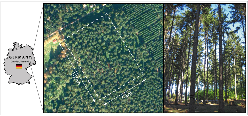
Figure 1.
Aerial and terrestrial view of the Study area Tharandt.
3.2. Terrestrial Laser Scanning Data
The TLS measurements were performed with a phase shift scanner (Z+F IMAGER® 5006i) in late September 2011. The scanner was selected because of its large field of view (FoV) (Hz: 360°, V: 310°) and the high scanning speed [31]. The in situ measurements were georeferenced based on two geodetic networks of control points. The first order network was realized with control points measured with a total station and RTK-GPS. A traverse, connecting four GPS control points with minor shadowing from the forest canopy, was introduced across the study area to be able to georeference the dataset. The second order network was realized with 32 spherical and 13 planar targets, which were placed across the study area (Figure 2). The planar targets, which consist of a black and white pattern and an identification number, were mounted on trees along the border of the study area. The traverse itself and the positions of all planar targets were measured with a total station. The spherical targets, which were used as tie points, were built from lightweight materials (aluminum and Styropor®) and were labeled for better identification purposes in the post processing. The target center can be seen from all directions, which is not the case for flat targets that need reorientation to the scanner. The spherical targets were mounted stand alone up to approximately 2 m above the forest floor.
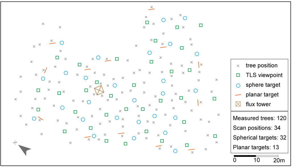
Figure 2.
Overview of the scanning geometry.
All TLS measurements were performed from the forest floor without using a lifting platform. The scan resolution was set to “Superhigh” which resulted in a point density of 16 points per cm2 at a distance of 10 m and a scan time of approximately 7 min per viewpoint when using the complete FoV of the scanner. The layout of the viewpoints for the scanning task was fixed in advance by marking potential viewpoints on site. At least four targets should be visible from each viewpoint and minimum shadowing as e.g., caused by too close tree stems should be given. In total, 34 scan positions, covering the complete study area, were measured in a two day campaign.
4. Methods
The first two steps consist of data acquisition and transformation of all scans from the sensor to the world coordinate system (WCS). In step 3, maps are generated showing the range and intensity measurements in the sensor coordinate system. Step 4 is the digitization of the axis of stem and branches and the radius determination from a single scan. These data are transformed to the WCS in step 5. In step 6, this tree model is transformed into a local coordinate system of another scan and displayed together with the maps in a new run through step 4. The sequence 6-4-5 is repeated for all scans, possibly using each scan a number of times. In this way, the modeled scene is becoming more and more complete. In a last step, the skeletonized tree structure is transformed to the WCS and extruded to a volumetric model. The suggested method is presented in an overview in Figure 3. The important steps will be presented in more detail below.

Figure 3.
General workflow of the presented method.
4.1. Registration of the Scans
Based on the GPS and total station measurements a geodetic network is derived with a free adjustment [32], using the GPS control points of the first order network as a reference. Furthermore, all scans are relatively and absolutely georeferenced by a least squares adjustment, using the control points and target positions picked in the different scans. As a result, for each viewpoint the transformation parameters from the scanners own coordinate system (SOCS) to the WCS are obtained. Finally, each scan is exported in SOCS in full resolution containing the coordinates plus intensity information.
4.2. Equirectangular Projection
Starting point of the map generation are the angle, range, and intensity observations of each scan. This can either be exported from the scanner or computed from the SOCS point cloud in the following way for each scan.
Let (xj, yj, zj) be the 3D Cartesian coordinates in the WCS, each of which is corresponding to an intensity value ij and where j = 1, …, n is the number of points in the scan. The scan position, i.e., the point with a range measurement zero, is denoted as (x0, y0, z0).
In these equations, αj is an azimuth, βj an elevation angle and rj the range. They typically do not correspond exactly to the original angle observations because of inclination and arbitrary orientation with respect to the north direction. Computation of the Cartesian coordinates from the angles and ranges is:
where R is an orthogonal matrix. If the original angles are used, R describes the rotation from the SOCS to the WCS.
Range and intensity are considered as functions of α and β. The (αj, βj) points may be regularly or irregularly distributed. By interpolation using nearest neighbor, moving least squares, or another local interpolation method, the range map r(α, β) and the intensity map i(α, β) are generated. Data holes should not be bridged, but a NODATA value should be given. The interpolation is performed in a regular grid providing an image. The images are—by their definition—equirectangular projections of the measured ranges and intensities of each scan. The grid spacing should correspond to the angle increments during scanning in order to maintain the level of information. There is a linear relation between the rows and columns of the image and α and β. The world file mechanism [33] may be used to convert between row, column and α, β. Another convention is that the upper left pixel center = (0°, 90°) for hemispherical scanners and the grid width (in angular units) is stored in the file name.
Alternatively to the range map, the horizontal range map can be computed, which is defined as:
Vertical lines (straight tree stems) have a constant rH. Applying normalization (or correction by range) of the intensity is straight forward in this step too:
The spatial extent of the interpolated image is prescribed by the FoV of the laser scanner. If the focus is on a small area only, a restriction may be applied. For 360° azimuth coverage, however, a periodic continuation of the acquired data can be useful for viewing purposes:
This way, a tree that is situated at the beginning and ending of data acquisition is not cut apart, but visible in one piece. This can be used analogously for the intensity maps. For visualization of the range images, a color palette is suggested. The intensity images are visualized with a grey scale palette (as presented in Figure 4).
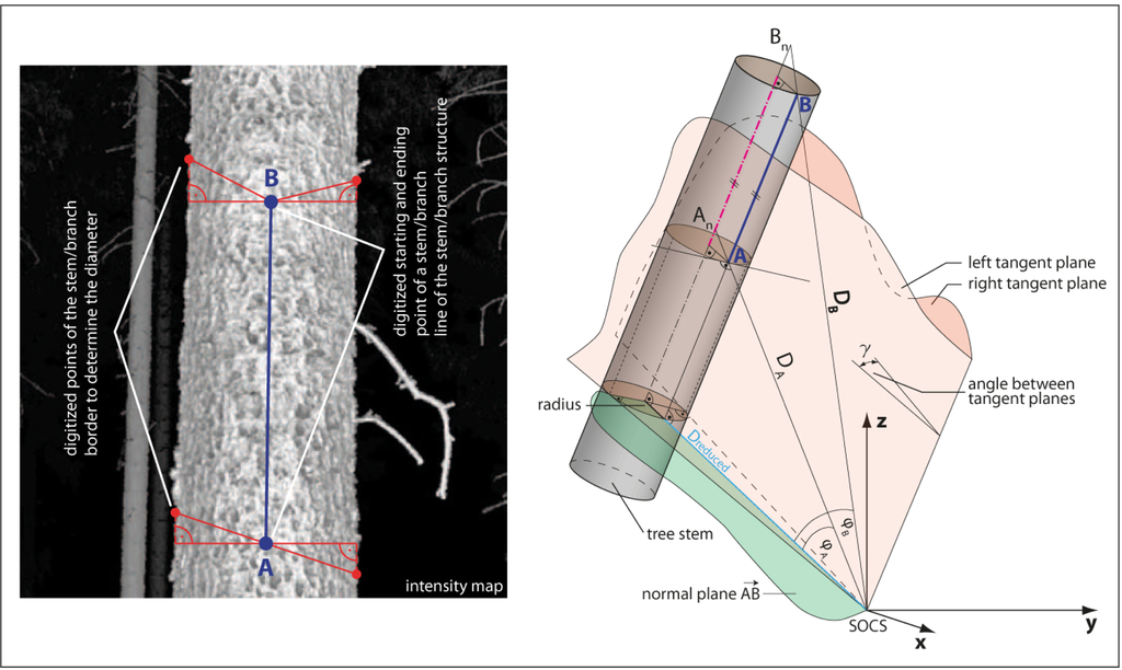
Figure 4.
Method for extracting tree topology based on digitizing in a 2D map. (Left) Digitization process based on the 2D intensity map; (Right) Geometrical relation for transferring the 2D measurements to 3D space.
4.3. Digitizing of Tree Axis Radius
The tree shall be described by the axis of the stem and the branches. As they are not necessarily straight but can be curved, multiple, connected line segments are used for modeling. For each segment, the local radius of the tree is defined.
For measuring the tree topology in a single scan a software supporting the digitization of line network, e.g., by providing object snapping, is required, e.g., a CAD or GIS. The basic digitization operation is measuring a line segment along the tree surface. The digitization may be performed in the range or intensity map. At the end points A and B of a segment, a point on the left and a point on the right stem/branch border are measured. These tangent points are used to obtain the diameter of the object. Figure 4 (left) shows the measurement process.
The axis of a branch segment and its radius correspond to a cylinder. The parameters of the cylinder, i.e., axis and radius, need to be determined robustly from the laser scanner measurements and the digitized points.
By measuring point A and B in 2D, the angles in the scanner coordinate system are determined via the transformation of the image coordinates (row and column) to the angles (α and β). The range is determined by the median of the range map values coming from the identified point and its 8-neighborhood. Therefore, points A and B can be transformed to a Cartesian coordinate system. The same procedure is performed for the tangent points picked at the edges of the object. For the tangent points no range information is determined. Using the left or right tangent points and the scanners origin the left and right tangential plane is derived (Figure 4 (right)). In a next step the normal plane of the Vector AB, including the scanners origin, can be derived. Next, the angles φA and φB are derived and furthermore the distances DA and DB are reduced to the normal plane since only in this normal plane a non distorted radius of the object is deducible. The radius r can be derived using:
where Dreduced is the shortest distance to the segment and γ is the angle between the tangent planes.
Based on the extracted radius r the Points A and B are shifted to the axis of the object. This axis element is in the middle of the tree, under the assumption of a circular cross section. Additionally the determined radius becomes an attribute of the axis segment.
This procedure is repeated for one map until all visible objects belonging to the tree topology are digitized by the interpreter. Line snapping ensures connection of consecutive axis segments.
4.4. Completion of Tree Model with Multiple TLS Viewpoints
The complete reconstruction of a tree cannot be performed from a single scan position as parts of the tree are occluded. Therefore, the tree topology is extracted stepwise from multiple scan positions. In this way, groups of trees are also completed stepwise. When all visible objects of a scan position are completely digitized, the extracted structure lines are transformed to the WCS. Then they are transformed into the coordinate system of the next scan to be processed for complementing the already extracted topology and new (previously occluded) trees. The lines can then be visualized as an overlay of the range and intensity maps of the new scan position. In addition to digitizing new axis segments, also existing ones may be improved.
4.5. Volumetric Modeling
After all scan positions are processed, the final skeletons of the trees are transformed to the WCS. To generate volumetric models of the digitized tree topology cylinders are generated for each line segment. Based on the starting and ending point of each line the axis of a cylinder is defined. The appropriate line attribute stored with each line is used to define the radius of the cylinder.
5. Implementation
5.1. Derived Base Products
As described above, for all scans an equirectangular projection (EP) based on the observation angles of the scan was created, thereby displaying the distances (range map, RM), intensity information (intensity map, IM), and the map showing the horizontal distances (horizontal range map, HM). Interpolation was performed with OPALS [34]. The spatial resolution of the maps was set to 0.018° which represents the angular step width of the scanning mode “Superhigh”. The maps show the full horizontal and vertical FoV of the scanner whereby pixels assigned to invalid TLS measurements are marked as NODATA. At the right edge of each map, the map was extended by appending the first, left quarter of the map. This should overcome limitations at the borders of the map to avoid having cut objects. For the IM grey scale coded maps and for the HM color coded maps were derived for visualization purposes, but the ranges themselves were also exported into a so called “Rangefile”, containing the ranges in ASCII.
5.2. Extraction of Tree Topology
The extraction of the tree topology was performed by digitizing stems and branches, visible in the intensity map and the map of horizontal ranges. AutoCAD was used for digitizing. While the images can be imported and displayed without problems in AutoCAD, the ranges needed special treatment. Image formats are restricted in AutoCAD, and therefore the full resolution float values of the ranges were imported into an array as an ASCII “Rangefile”. The conversions between the various coordinate systems and the extrusions of the final tree skeletons to cylinder models were performed with VBA scripts.
6. Results
6.1. Registration of the TLS Data
For the first order network a free network adjustment was performed separately for horizontal positions and height using the software package Geosi [35]. Based on the adjusted control points of the first order network and the tie points of the second order network 34 single scans were georeferenced. In each scan, at least six targets were visible for the laser scanner and were measured in the according SOCS during the data acquisition process. In a pre-processing step the 3D coordinates of all visible targets were manually picked in the according SOCS. This was performed using the software “Z+F Lasercontrol 8.2” [36]. The sphere centers were semi-automatically extracted using local sphere-fits within the point cloud. The centers of the planar targets were also semi-automatically extracted using a built in function provided by the software. Based on the reference measurements provided by the total station and the extracted target positions in the scans a 3D bundle block adjustment was performed to finally derive transformation parameters for each single scan. For the relative orientation, 323 targets were extracted from the scan data and were used in the bundle adjustment. For the absolute georeferencing 13 planar targets were used. The average deviation of the planar targets with respect to the total station data shows a value of 5 mm. The relative orientation shows an average target deviation of 4 mm. Each transformation parameter set allowed directly georeferencing of the scans from SOCS to the target system UTM33N. For each viewpoint, the TLS data was exported in ASCII XYZi format in the SOCS, containing the originally measured intensity values for each TLS point.
6.2. Equirectangular Projections
In general, objects close to the upper and lower edge of the maps are distorted. This is a general property of the equirectangular projection as explained by Tissot’s indicatrix. In the IM tree stems and branches are clearly visible. In the upper part of the map, wavy branches are partly visible which were moving due to wind influence during the data acquisition. With increasing distance from the scanners origin, the backscattered intensity decreases which results in darker grey tones for objects more than approximately 30 m away from the scanner. Due to the different reflective properties of the targets the structure of the forest floor and the stems’ bark is visible. Additionally when focusing on living branches the wooden part is distinguishable from the foliage in most cases. The spatial resolution of the processed map is high enough to visualize even small branches of trees, closer than approximately 20 m to the scanner. The beam diameter of the scanner’s laser is approximately 2–7 mm depending on the range. The point spacing of the TLS measurements is theoretically 1.6 mm at a range of 5 m, 4.7 mm at a range of 15 m and up to 8 mm at a range of 25 m. Based on the given scan parameters branches with a minimum diameter dmin of 4 mm (scanning range within 5 m), 1 cm (scanning range within 15 m) or 1.5 cm (scanning range up to 25 m) are visible in the maps as continuous pixel bands. Considering the distance calculation as presented in Section 4.3 the minimum reconstructable branch diameter digitmin is determined by:
where 5/9 is coming from the median distance calculation within the 3 × 3 kernel. Therefore, the theoretically extractable minimum branch diameter is 6 mm for a distance within 5 m, 1.6 cm for a distance within 15 m and 3.1 cm within a distance of 25 m.
The HM has the same geometrical properties as the IM. The differently colored horizontal distances allow a clearer separation of trees standing at different ranges. This is especially useful if different branches at different ranges partly overlap in the map.
Figure 5 shows the resulting IM and HM of one scan position.
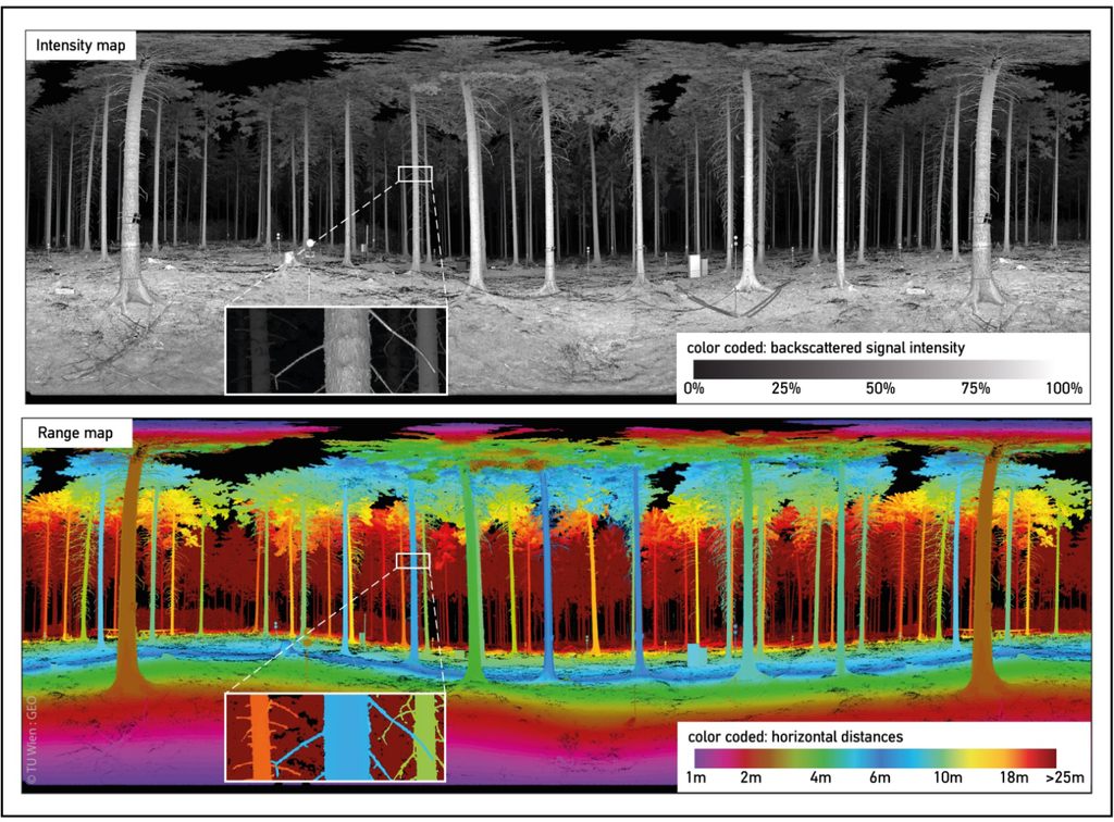
Figure 5.
Color coded intensity map and range map (horiz. distances) of a single scan position.
6.3. Digitized Tree Topology
The digitization result for a single scan shows a set of lines, which follow the axes of the stems and branches. To detect and correct misinterpreted points, the interpreter carried out intermediate checks within the digitization process. This was done by transforming the 2D lines to 3D space and visually checking the generated lines. Additionally the newly digitized lines were visually checked after transforming them to another scan position. In the final 2D digitization of one scan position the starting and ending points of corresponding neighboring lines are correctly connected. Lines that represent a connection between a stem and a branch are correctly intersected with the line that represents the stem. In many cases, partly occluded areas could be bridged over in the digitization process which is attributable to the expert knowledge of the interpreter. In general, the upper part of a tree is easier to digitize if the tree is located more than approximately 6 m away from the scan position. The reconstruction of the top most part of the stem/branch structure is limited due to big data gaps of the TLS measurements and distortions of the maps. Therefore, usually, only segments of branches can be digitized in one scan, but completion of full branches can be done in other scans. Lines from already interpreted scan positions are correctly transformed and furthermore displayed in the target map of a different scan position (Figure 6). The digitized lines were transformed 66 times in total between different scan positions. Corresponding neighboring lines as well as intersected lines of the tree skeletons are correctly connected in 3D after the final transformation into the WCS. The time needed for modeling a single tree is hard to estimate as the digitized trees are composed of lines digitized from multiple scan positions and the trees differ in their appearance. A rough estimate can be given with 30 to 45 min per tree.
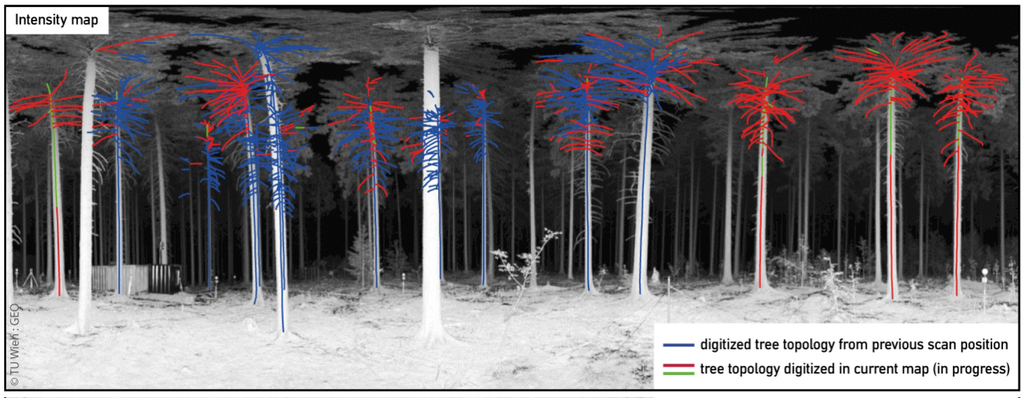
Figure 6.
Digitized tree topology overlay with the intensity map. The blue color indicates the structure extracted from a previous scan position. Red and green colors indicate lines that are digitized in the current map.
6.4. Volumetric Models
A visual inspection of the volumetric models shows that all cylinders are extruded correctly from the information stored with the 3D lines, containing the corresponding line segment as its axis. In total 38,101 cylinders were extruded from the tree skeletons representing 90 trees (Figure 7). The smallest modeled cylinder shows a diameter of 7 mm, the largest cylinder modeled shows a diameter of 1.05 m. A visual inspection of the final modeled scene and five randomly selected single trees shows that the stems and branches could be modeled approximately up to three quarters of the tree height and the determined cylinders show a good agreement with the corresponding point cloud (Figure 8). In the upper section of the trees, the modeled branches start to get fragmented and in most cases they are not connected to a stem. For neighboring cylinders, no rapid diameter changes or rapid, unnatural changes of the orientation of the cylinders are visible. Only at the very bottom of some stems a rapid change of the diameter is visible which seams plausible as many tree stems widen up at this area for stabilization purposes.
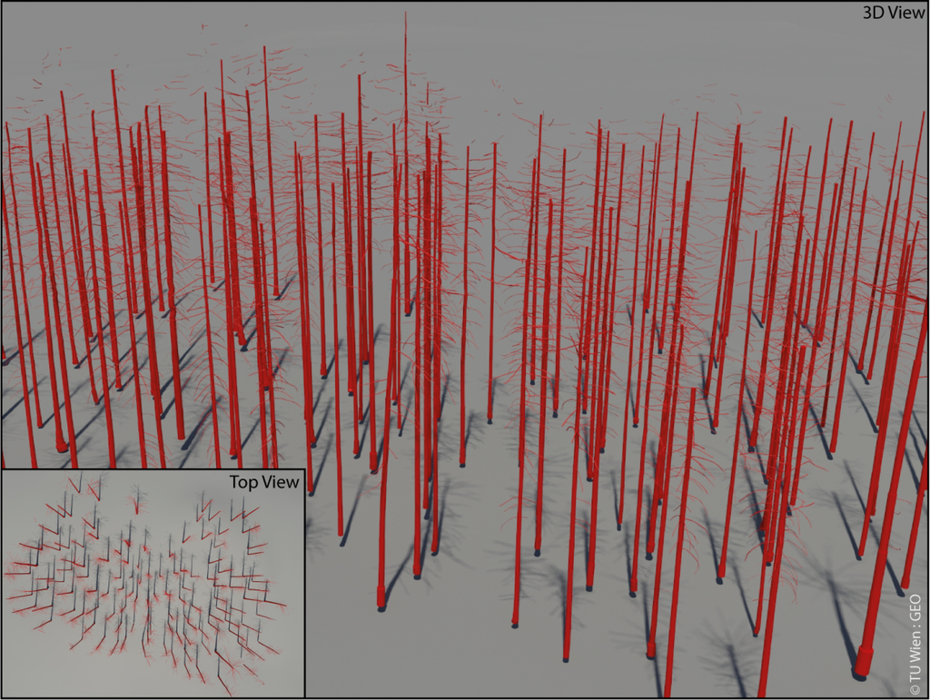
Figure 7.
3D visualization of the reconstructed forest stand.
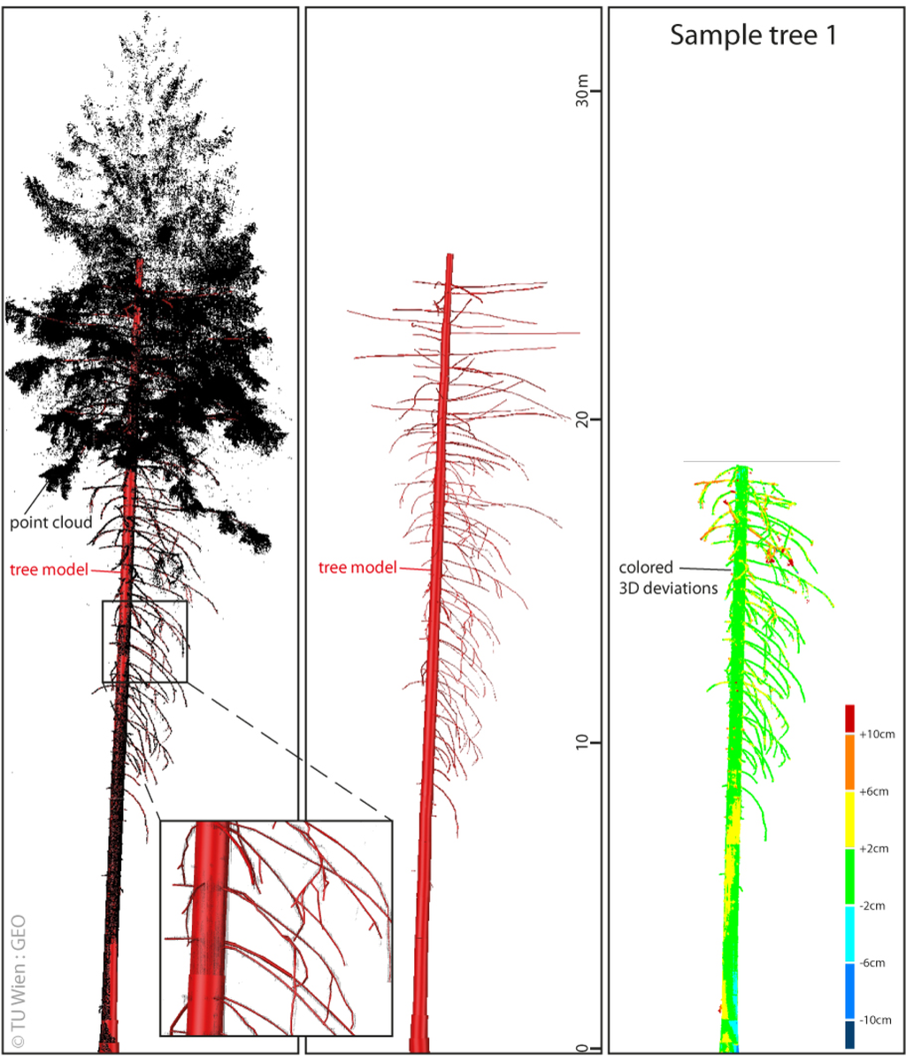
Figure 8.
Extracted tree model of sample tree 1; (Left) Extracted tree model versus merged TLS point cloud; (Middle) Extracted tree model; (Right) 3D Deviations.
6.5. Validation
The quality of the modeled trees is validated based on five randomly selected trees from the scene. Each tree model is tested in two different ways against the corresponding point cloud.
Validation Method 1 investigates the stem diameters of the modeled trees by cutting horizontal slices from the point cloud and the model. The thickness of the slices is set to 1 cm and the spacing between the slices was set to 1 m (Figure 9). For each slice the stem diameter of the model (DMODEL) and the mean stem diameter from the TLS point cloud (DTLS) are determined. DTLS is deduced by deriving the mean value of two stem diameter measurements performed in the sliced point cloud. Figure 9 shows the resulting stem/trunk diameter profiles of the sample trees. In total 71 slices were analyzed. All profiles show decreasing DMODEL and DTLS values with increasing height above ground. The mean of residuals between DMODEL and DTLS shows values between −1.3 cm and 1.7 cm. The standard deviation of residuals shows values between 0.9 cm and 2.0 cm.
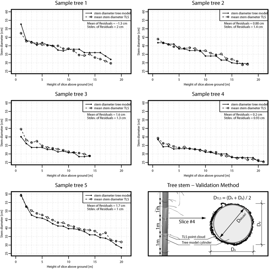
Figure 9.
Validation Method 1. Validation of the stem performed for five randomly selected sample trees. Based on horizontal slicing of the point cloud and the model the diameters of the stem are determined. The stem diameters are plotted against the height of the slices above ground as stem profiles.
Validation Method 2 investigates the 3D deviations between the models of the sample trees and their corresponding TLS point clouds to test the model for completeness and correctness. Since only the wooden parts of the trees should be investigated the point clouds were manually edited in a pre-processing step. In this step, ground points and all points above the first living branch were deleted. Based on the edited point clouds the 3D deviations were derived for each tree. The 3D deviations of sample tree 1 are displayed in Figure 8 colored by a color spectrum. Histograms of the deviations are presented in Figure 10. The mean of deviations for all trees are between 0.2 cm and 0.6 cm. The standard deviations for all trees are between 1 cm and 2 cm.
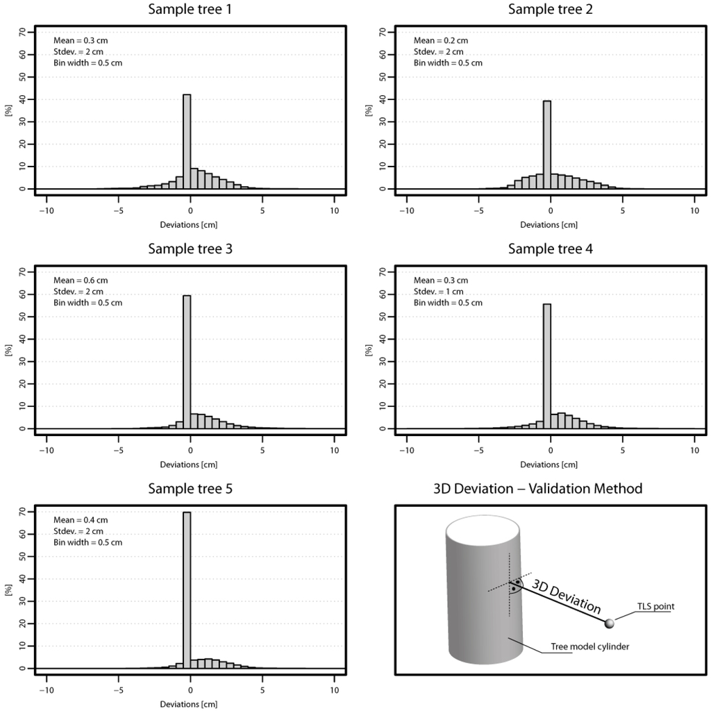
Figure 10.
Validation Method 2. Validation of five randomly selected sample trees by investigating the 3D deviations between the TLS point cloud and the model. Histograms of the deviations are presented for each tree.
7. Discussion
The result of the presented semi-automatically method shows that the reconstruction of tree topology based on a simple digitization is possible with a high level of detail. As parts of the structure of a tree (stem, branches) are clearly interpretable in the introduced high resolution maps, these maps provide a good basis for extracting the tree structure by digitizing the axis of the structure elements in 2D. This is an advantage compared to the method described by Dassot et al. [12]. The digitization can be performed in the intensity map and/or in the range map, using the advantages of the different image information. The intensity map shows the distance corrected backscattered signal intensities and clearly visualizes the wooden part of a tree. The horizontal distances shown in the range map allow the interpreter to separate tree topology of trees standing at different ranges. The image distortions at the upper part of the maps as well as occlusion effects limit the digitization of the upper tree parts. Therefore, trees standing further away from the scan position are better suited for digitizing the tree’s upper part, depending on the visibility. The visibility mainly depends on the density of the scan data and the density of the branches/needles. Other projections or scan positions performed from a lifting platform may help to overcome this limitation. Also the time of the year can make a huge difference for the data acquisition as for example some trees loose their leaves or needles in fall which might be an advantage for the field campaign. Due to the expert knowledge of the interpreter, data gaps can be overcome during the digitization process. Depending on the local situation larger gaps greater than approximately 1 m can be bridged in many cases. This is an advantage compared to fully automatic algorithms as e.g., presented by Pfeifer et al. [19], Raumonen et al. [28] or Bucksch [17]. It should be noted that the bridgeable gap size is depending on the local situation, i.e., point density, degree of occlusion, wind effects, etc.
The tree topology is extracted step wise from multiple scan positions. In this way partly occluded branches and furthermore groups of trees are completed stepwise. Imperfections of the merged point cloud, caused by remaining registration errors, noise or i.e., moving branches which were influenced by wind, are overcome in most cases because of the digitization method (Figure 11).
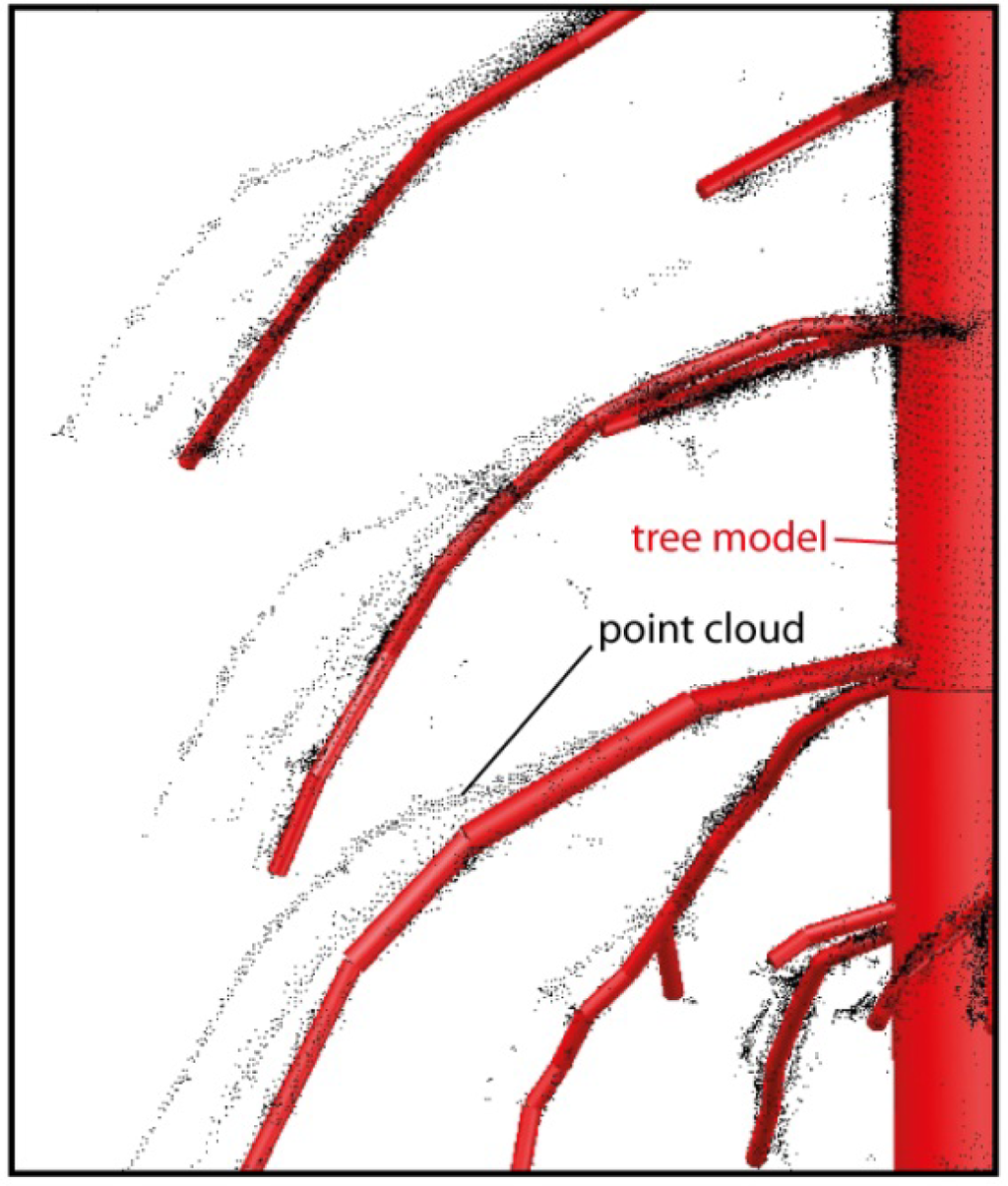
Figure 11.
Tree model versus merged point cloud. The merged point cloud, merged from three different scans, shows multiple positions for the same branch due to wind influence.
This is an advantage compared to voxel methods, which are based on a merged pointcloud e.g., [15,16,18]. One of the big benefits of using single scans and their projections is that the inevitable systematic errors (imperfect registration) and random errors (noise) are an unsolvable problem. In forest scans, there are always “phantom points” which are generated from multiple returns and they are along the same line from the scanner. In 3D, these points are visible and problematic, but in 2D projections these all have the same projection and thus they are not visible. Therefore, no filter steps are necessary. This is an advantage over methods that rely on a filtered pointcloud, e.g., [15–17,28].
Additionally, the step wise reconstruction also ensures the quality of the final model. Because the already reconstructed lines are plotted in a new scan, the interpreter visually checks the alignment of the axis with the trees in a new view. Gross errors, e.g., a wrong range measurement, immediately become visible. The cylinders of the extruded volumetric models show no rapid diameter changes or unnatural direction changes and correctly represent the point cloud in its close vicinity in most cases. In contrast to the method presented by Côté et al. [23], all branches of the tree models follow the “original” branch structure as no branch colonization algorithm is used. This is also reflected in the validation results presented in Section 6.5. For the tested trees/stems the standard deviation of residuals (Stem diameters Model against stem diameters TLS) varies between 0.9 cm and 2.0 cm. The tested 3D deviation (Tree model against TLS point cloud) shows standard deviations between 1.0 cm and 2.0 cm. The validation proves that the lower part of the trees is modeled correctly and completely. This is also supported by the histogram of 3D deviations presented in Figure 10 and the colorized 3D deviations presented in Figure 8. Primarily wind and registration errors cause large deviations. For the upper part a validation is very challenging and could not be performed within this work. No reference measurements of upper tree parts are available as the trees are too tall. A destructive validation method as for example presented in Dassot et al. [12] was not an option, as the trees cannot be cut down. Validating the method by investigating an artificial tree as presented in Raumonen et al. [28] was not an option because the simulated point cloud doesn’t consider the influence of wind, visibility especially in the upper part of the tree and imperfect point clouds from different TLS viewpoints due to limitations in the registration. Thus, such a simulated point cloud doesn’t sufficiently represent the real situation in a dense forest stand with a mean tree height of approximately 30 m. A validation based on tree height and a single DBH measure as presented in Vonderach et al. [15] was assumed to be insufficient as the information about completeness and correctness is limited. Furthermore, this publication investigated deciduous trees under leave-off conditions in an urban environment. In general, a comparison between results from different approaches is limited as most authors studied single trees, e.g., [15,18,19,37]. Therefore, a good visibility during the data acquisition was possible resulting in point clouds with a high completeness. In contrast, a dense forest stand is investigated in this study resulting in incomplete point clouds. Another aspect is that many authors study deciduous trees under leave-off conditions. In most cases, the tree heights of the studied trees are much lower than the ones presented in this study, e.g., [12,14–16,18]. Therefore a different scanning geometry and a different point density is given for the upper part of the trees in these studies. A throughout comparison of different modeling approaches is limited since no standard dataset on trees is available nor is there a common method of evaluation. In Raumonen et al. [28] a 22 m high Norway spruce (Picea abies (L.)) was scanned and further on modeled under leave-on conditions. The tree model and TLS data in Raumonen et al. [28] is comparable to the tree models/TLS data from this study. Raumonen et al. [28] discuss that the missing data in the upper part of the tree affects the modeling of the upper part, which can be seen in the resulting model. Their resulting model is successfully reconstructed to approximately three quarters of the total tree height. This result is comparable to the results presented in this study.
Regarding modeling of small branches, the minimum modeled diameter is 7 mm. This value is supported by the resolution of the equirectangular maps and the resulting theoretically extractable radius as presented in Section 6.2. Obtaining such a small diameter seems to be realistic for objects closer than approximately 5 m to the scanner. In general mixed pixels and resulting noise in the TLS measurements limits the modeling of small branches. Wind does not affect the extraction of small branches but it limits their accuracy. It is assumed that a minimum extractable diameter of 1 to 3 cm is realistic for branches larger than 5 m away from the scanner. This value depends on the objects distance to the scanner and the environmental conditions. Similar values are reported in Raumonen et al. [28].
Focusing on the TLS data the quality of the acquired data was sufficient for reconstructing the forest scene with a high level of detail. The chosen acquisition and registration strategy delivered well aligned scans, which is crucial for the presented reconstruction method. The resulting tree models look realistic and represent the trees of the dense forest stand up to approximately three quarter of the total individual tree height. Problems with the reconstruction of the uppermost part of a tree are also discussed by other authors (e.g., [19,23,28]). This is mainly caused by imperfections and large data gaps within the point cloud.
The presented method can be improved in a number of ways. A combination with very dense, well aligned airborne laser scanning data acquired by low flying drones or TLS scans carried out from a lifting platform may help to overcome some of the limitations. Alternative map projections may be applied (e.g., stereographic projection for areas close to the zenith). True colored terrestrial laser scans could help the interpreter to distinguish between wooden tree parts and foliage. Given the digitization on the tree surface, larger branches and the stem can be reconstructed by cylinder fitting rather than extracting the radius within the digitization process. Furthermore, the most challenging aspect of automation is obtaining a complete skeleton. Advancing from an approximate skeleton to the axis reconstruction will reduce the need for following curved branches with multiple digitized points. Because of imperfect point clouds (wind, etc.), we see a limit in the automation for larger scenes.
In respect to the application of the reconstructed 3D models within the project 3D Vegetation Lab [3], radiative transfer modeling, the accuracy of the presented method is sufficient, as it only covers the stems and major branches. The use of cylinders for tree model representation is well established in radiative transfer modeling, thus the generalization applied in this study is valid. To complete tree models augmenting the structure in the upper parts with synthetic models and populating it with foliage is necessary. For example in Eysn et al. [5] shoots were modeled based on triangulating scanner data and cloned across the tree model to simulate the entire tree crown. Additionally radiometric properties can be assigned to the geometric models as shown in Côté et al. [37], which provide an appropriate input dataset for radiative transfer modeling.
8. Conclusions
We presented a method for reconstructing 3D tree models based on terrestrial laser scanning data of a forest scene. The trees are modeled by semi-automatically digitizing the wooden parts (i.e., branching and stem structure) in 2D maps. Each tree is described by the axis of its stem and branches and the corresponding radius. The 2D maps are equirectangular projections of the terrestrial laser scanning data showing the range and the intensity measurements of the scanner respectively. The modeling is performed for each viewpoint individually instead of using a merged point cloud, whereas previously reconstructed 2D-skeletons are transformed between the maps. In the final model, the digitized tree skeletons are extruded to cylinders by using the obtained radii.
Due to the requirements of this method to achieve a high completeness and correctness we rely on human interpretation capabilities rather than applying entirely automated approaches. The presented methods therefore focus on enabling simple navigation in the data using 2D maps and incremental completion by using multiple scans. Imperfections of the merged point cloud, caused by remaining registration errors, noise or, i.e., moving branches which were influenced by wind, are mitigated in most cases because of the proposed digitization method. Bridging of gaps may be performed by the operator, but extrapolation or growing of tree structure is not within the scope of this approach.
The main limiting factors for the proposed modeling method are the quality of the TLS data, the visibility of the upper tree parts during the data acquisition and distortions in the 2D maps originating from the chosen projection. These limitations except the last one apply to all reconstruction methods presented in the literature. Summarizing, with the existing approaches our method shares the limitation of reduced visibility in the upper tree parts due to the scan position, it provides better handling of registration errors and wind distortions in the point cloud, a current limitation specific for this method is that areas close to the zenith are not mapped well, and it integrates manual interpretation.
The approach was applied to a terrestrial laser scanning dataset from a managed dense forest stand in Germany. 90 coniferous trees were reconstructed with their stem and branches as visible in 34 single scans. For conifers the occlusions towards the tree tops are limiting the reconstruction. The single trees were modeled up to three quarters of the total tree height. In total 38,101 cylinders were modeled to represent the complete stand. The minimum cylinder diameter modeled shows a value of 7 mm.
The quality of the modeled trees was tested on five randomly picked sample trees. A validation of horizontal slices of the stems by investigating residuals between tree model and scan data shows values between −1.3 cm and 1.7 cm. Additionally a new validation method is proposed to test the models for completeness and correctness. All wooden and defoliated parts of the tree were investigated by deriving the 3D deviations between tree model and point cloud. Standard deviations of the 3D deviations of approximately 1.0 cm were found. In the literature, a high variety of different scanning datasets and validation strategies can be found which makes a qualitative intercomparison challenging. Consequently, there is a need for a standardized validation strategy and input dataset respectively.
In the future the presented method will be developed further, for example by investigating different map projections or automatically extracting the axis of the wooden tree elements from the 2D maps to speed up the digitization process. A standardized benchmark together with other tree modeling approaches is also considered as a future task.
Acknowledgments
This study is partly financed by the ESA funded 3D-VegetationLab project and the project NEWFOR financed by the European Territorial Cooperation “Alpine Space”. We thank Werner Mücke and Franz Blauensteiner for performing the in situ TLS measurements.
Conflicts of Interest
The authors declare no conflict of interest.
References
- ESA European Space Agency (ESA). Available online: http://www.esa.int/ESA (accessed on 19 November 2012).
- ESA European Space Agency (ESA)—Living Planet Programme—Gmes. Available online: http://www.esa.int/esaLP/SEMM4T4KXMF_LPgmes_0.html (accessed on 20 November 2012).
- ESA 3D Vegetation Lab. Available online: http://due.esrin.esa.int/stse/projects/stse_project.php?id=139 (accessed on 20 November 2012).
- Lovell, J.L.; Jupp, D.L.B.; Newnham, G.J.; Culvenor, D.S. Measuring tree stem diameters using intensity profiles from ground-based scanning lidar from a fixed viewpoint. ISPRS J. Photogramm. Remote Sens 2011, 66, 46–55. [Google Scholar]
- Eysn, L.; Ressl, C.; Grafl, A.; Hollaus, M.; Mücke, W.; Morsdorf, F.; Pfeifer, N. Extraction of 3D Tree Models Based on Equirectangular Projections of Terrestrial Laser Scanning Data. Proceedings of SilviLaser 2012, Vancouver, BC, Canada, 16–19 September 2012.
- Biliouris, D.; van der Zande, D.; Verstraeten, W.; Muys, B.; Coppin, P. Assessing the impact of canopy structure simplification in common multilayer models on irradiance absorption estimates of measured and virtually created Fagus sylvatica (L.) stands. Remote Sens 2009, 1, 1009–1027. [Google Scholar]
- Xinlian, L.; Litkey, P.; Hyyppa, J.; Kaartinen, H.; Vastaranta, M.; Holopainen, M. Automatic stem mapping using single-scan terrestrial laser scanning. IEEE Trans. Geosci. Remote Sens 2012, 50, 661–670. [Google Scholar]
- Hopkinson, C.; Chasmer, L.; Young-Pow, C.; Treitz, P. Assessing forest metrics with a ground-based scanning lidar. Can. J. For. Res 2004, 34, 573–583. [Google Scholar]
- Maas, H.G.; Bienert, A.; Scheller, S.; Keane, E. Automatic forest inventory parameter determination from terrestrial laser scanner data. Int. J. Remote Sens 2008, 29, 1579–1593. [Google Scholar]
- Tansey, K.; Selmes, N.; Anstee, A.; Tate, N.J.; Denniss, A. Estimating tree and stand variables in a corsican pine woodland from terrestrial laser scanner data. Int. J. Remote Sens 2009, 30, 5195–5209. [Google Scholar]
- Bienert, A.; Scheller, S.; Keane, E.; Mohan, F.; Nugent, C. Tree Detection and Diameter Estimations by Analysis of Forest Terrestrial Laserscanner Point Clouds. Proceedings of ISPRS Workshop on Laser Scanning 2007 and SilviLaser 2007, Espoo, Finland, 12–14 September 2007; pp. 50–55.
- Dassot, M.; Colin, A.; Santenoise, P.; Fournier, M.; Constant, T. Terrestrial laser scanning for measuring the solid wood volume, including branches, of adult standing trees in the forest environment. Comput. Electron. Agric 2012, 89, 86–93. [Google Scholar]
- Schilling, A.; Schmidt, A.; Maas, H.G. Tree topology representation from TLS point clouds using depth-first search in voxel space. Photogramm. Eng. Remote Sens 2012, 78, 383–392. [Google Scholar]
- Delagrange, S.; Rochon, P. Reconstruction and analysis of a deciduous sapling using digital photographs or terrestrial-lidar technology. Ann. Bot 2011, 108, 991–1000. [Google Scholar]
- Vonderach, C.; Vögtle, T.; Adler, P.; Norra, S. Terrestrial laser scanning for estimating urban tree volume and carbon content. Int. J. Remote Sens 2012, 33, 6652–6667. [Google Scholar]
- Hosoi, F.; Nakai, Y.; Omasa, K. 3-D voxel-based solid modeling of a broad-leaved tree for accurate volume estimation using portable scanning lidar. ISPRS J. Photogramm. Remote Sens 2013, 82, 41–48. [Google Scholar]
- Bucksch, A. Revealing the Skeleton from Imperfect Point Clouds. Delft University of Technology, Delft, The Netherlands, 2011. [Google Scholar]
- Bucksch, A.; Lindenbergh, R.; Menenti, M. SkelTre. Vis. Comput 2010, 26, 1283–1300. [Google Scholar]
- Pfeifer, N.; Gorte, B.; Winterhalder, D. Automatic Reconstruction of Single Trees from Terrestrial Laser Scanner Data. Proceedings of the XXth ISPRS Congress: Geo-Imagery Bridging Continents, Istanbul, Turkey, 12–23 July 2004; pp. 114–119.
- Thies, M.; Pfeifer, N.; Winterhalder, D.; Gorte, B.G.H. Three-dimensional reconstruction of stems for assessment of taper, sweep and lean based on laser scanning of standing trees. Scand. J. For. Res 2004, 19, 571–581. [Google Scholar]
- Gorte, B.; Pfeifer, N. Structuring Laser-Scanned Trees Using 3D Mathematical Morphology. Proceedings of the XXth ISPRS Congress: GeoImagery Bridging Continents, Istanbul, Turkey, 12–23 July 2004; pp. 929–933.
- Palágyi, K.; Tschirren, J.; Sonka, M. Quantitative Analysis of Intrathoracic Airway Trees: Methods and Validation. In Information Processing in Medical Imaging; Taylor, C., Noble, J.A., Eds.; Springer: Berlin/Heidelberg, Germany, 2003; Volume 2732, pp. 222–233. [Google Scholar]
- Côté, J.-F.; Fournier, R.A.; Egli, R. An architectural model of trees to estimate forest structural attributes using terrestrial lidar. Environ. Model. Softw 2011, 26, 761–777. [Google Scholar]
- Verroust, A.; Lazarus, F. Extracting Skeletal Curves from 3D Scattered Data. Proceedings of International Conference on Shape Modeling and Applications (Shape Modeling International ’99), Aizu, Japan, 1–4 March 1999; pp. 194–201.
- Runions, A.; Lane, B.; Prusinkiewicz, P. Modeling Trees with a Space Colonization Algorithm. Proceedings of Eurographics Workshop on Natural Phenomena, Prague, Czech Republik, 4 September 2007.
- Palubicki, W.; Horel, K.; Longay, S.; Runions, A.; Lane, B.; Mech, R.; Prusinkiewicz, P. Self-organizing tree models for image synthesis. ACM Trans. Graph 2009, 28, 1–10. [Google Scholar]
- Cheng, Z.; Zhang, X.; Fourcaud, T. Tree Skeleton Extraction from a Single Range Image. Proceedings of Second International Symposium on Plant Growth Modeling and Applications (PMA ’06), Beijing, China, 13–17 November 2006; pp. 274–281.
- Raumonen, P.; Kaasalainen, M.; Åkerblom, M.; Kaasalainen, S.; Kaartinen, H.; Vastaranta, M.; Holopainen, M.; Disney, M.; Lewis, P. Fast automatic precision tree models from terrestrial laser scanner data. Remote Sens 2013, 5, 491–520. [Google Scholar]
- Dassot, M.; Constant, T.; Fournier, M. The use of terrestrial lidar technology in forest science: Application fields, benefits and challenges. Ann. For. Sci 2011, 68, 959–974. [Google Scholar]
- Bucksch, A.; Khoshelham, K. Localized registration of point clouds of botanic trees. IEEE Geosci. Remote Sens. Lett 2013, 10, 631–635. [Google Scholar]
- Zoller+Fröhlich Technical Data z+f IMAGER 5006i. Available online: http://sluzby.geodis.cz/uploads/dokumenty/laserove_skenovani/Datenblatt_IMAGER5006i_E.pdf (accessed on 22 November 2012).
- Brinker, R.C.; Minnick, R. The Surveying Handbook; Springer-Science+Business Media, B.V.: Dordrecht, The Netherlands, 1995; p. 971. [Google Scholar]
- ESRI Understanding World Files. Available online: http://webhelp.esri.com/arcims/9.2/general/topics/author_world_files.htm (accessed on 9 April 2013).
- OPALS Orientation and Processing of Airborne Laser Scanning Data. Available online: http://www.geo.tuwien.ac.at/opals/ (accessed on 19 November 2012).
- IDC Software Package Geosi Netz. Available online: http://www.geosi.at/index.php?id=78&L=0 (accessed on 22 November 2012).
- Zoller+Fröhlich Software Package Z+F Laser Control 8.2. Available online: http://www.zf-laser.com/Z-F-LaserControl.132.0.html (accessed on 9 April 2013).
- Côté, J.-F.; Widlowski, J.-L.; Fournier, R.A.; Verstraete, M.M. The structural and radiative consistency of three-dimensional tree reconstructions from terrestrial lidar. Remote Sens. Environ 2009, 113, 1067–1081. [Google Scholar]
© 2013 by the authors; licensee MDPI, Basel, Switzerland This article is an open access article distributed under the terms and conditions of the Creative Commons Attribution license ( http://creativecommons.org/licenses/by/3.0/).