4.1. LiDAR Model
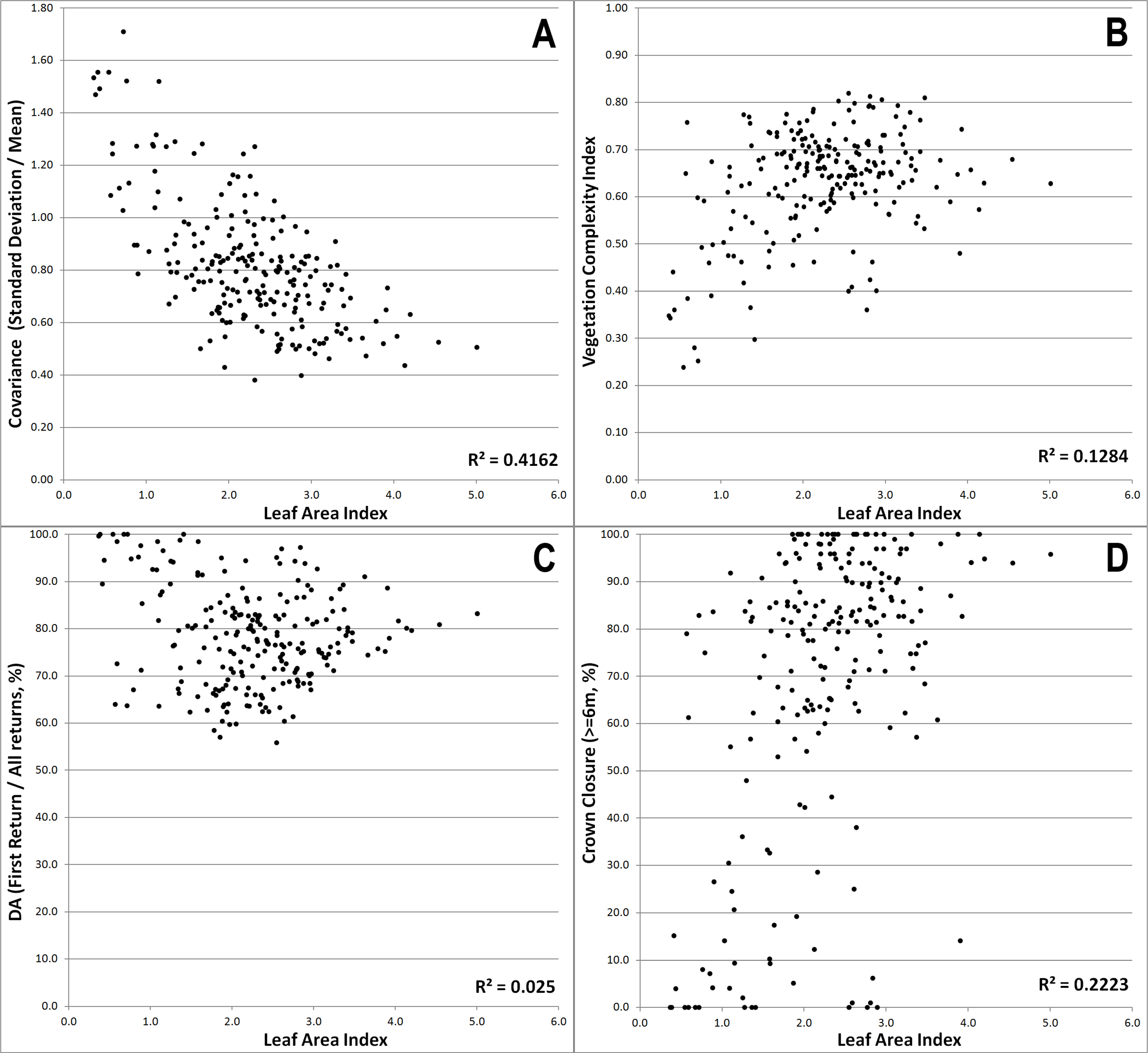
The inclusion of the four final variables presented above suggests some interesting aspects about the model and LiDAR prediction of LAI in general. The COVAR exhibited a strong, negative correlation to LAI (R
2 = 0.42),
i.e., as LAI increased, COVAR decreased (
Figure 12A). High COVAR corresponds to high standard deviation (
i.e., more open, penetrable, variable canopies), and/or low mean height (
i.e., shorter, immature trees). It was anticipated that a variable of this nature would be included in the final model since it is a coarse surrogate for gap fraction (
i.e., greater penetration = higher gap fraction = lower LAI). In laboratory controlled experiments with high density laser scanners and artificial trees it has been shown that increased leaf count corresponds to a decrease in pulse return density at greater distances into the canopy, thereby increasing standard deviation [
36].
Other predictor variables did not exhibit strong correlations to LAI. However, the nature of MLR is that the combination and interplay of trends between predictor variables can often generate more explanatory power than an individual variable.
Figure 12B illustrates the relatively weak positive correlation between LAI and VCI. VCI is a variable similar to COVAR, in that it is a measure of the structural complexity of the forest canopy, but inverse to COVAR, as high VCI corresponds to high LAI (
i.e., multi-layered forest canopy) [
37].
DA (
i.e., first return divided by all returns) was another variable that linked closely to the concept of gap fraction and how much penetration a canopy allows [
36]. As the number of first returns was equal to the total number of laser pulses transmitted (
i.e., a near-constant value for each equal area plot), the only changing variable in DA was the total number of returns. If the canopy is dense, the pulse is occluded and there is a higher chance of the first return being the only return; more open canopies allow for greater pulse penetration and a higher chance of two or three returns. The expected relationship was therefore that higher DA values are indicative of higher LAI. That trend was not observed clearly with this dataset, as there were many low LAI values which actually had the highest DA value (
Figure 12C). It was observed that in non-vegetated, completely open areas the same high DA values can be seen, given first returns (
i.e., only returns) were ground returns. Since this dataset contained only plots that were vegetated to some degree, a non-linear relationship would not be expected, but this trend may be partially responsible for odd artifacts in clear-cut areas in the complete forest LAI estimate surface.
Crown closure (≥6 m; cc6) was the predictor variable most unlike the others as it was not a measure of statistical spread or the direct complexity of the canopy. Crown closure at each height was calculated as a proportion of the number of 2 m sub-pixels within the 20 m pixel that matched the height criteria to the total number of pixels (
i.e., 100). As a measure of how closed the canopy was looking down from above to a certain height, cc6 was an interesting substitute for gap fraction. This trend shows that higher LAI corresponds to greater crown closure at six meters and above (
Figure 12D). The basis of this relationship is that for the plots investigated, six meters is below a significant portion of the canopy, and is definitely above understory vegetation. Maximum tree height in each plot is close to 15 m, so all vegetation greater than six meters is a good indication of total crown closure. This particular relationship compares especially well with the LAI values as the camera system was mounted 1.3 m from the ground and processing eliminated a conical field of view 18° above the horizon. Selecting six meters as the particular height to use from the suite of two meter intervals was done through the same step-wise methods as the primary model. Six meters was chosen as the variable from the low height ranges (
i.e., two–eight meters) that had the most explanatory power in the model.
The lack of height (P‘XX’) and density (D‘X’) metrics captured in the model was noteworthy as these tend to be predominant in modeling many other forest inventory variables (e.g., biomass, height, density) (e.g., [
23,
38,
39]). This absence likely stems from the fact that although the P‘XX’ and D‘X’ variables do give a general measure of canopy penetration and complexity, there were other variables in the LiDAR suite that were better surrogates for canopy gap fraction. Rough trials using only basic height and density metrics as potential inputs to a stepwise model proved that satisfactory models could be created, albeit at lower R
2’s (e.g., 0.40–0.45). The lower accuracy may be an acceptable trade-off for users hoping to generate more basic, easily interpretable models, where simplicity could outweigh a small level of error. Overall, this portion of the study provides interesting insight into the relationships between these height and density metrics and variables more related to overall canopy characteristics and crown closure. LAI seems to be more reliably estimated with the latter.
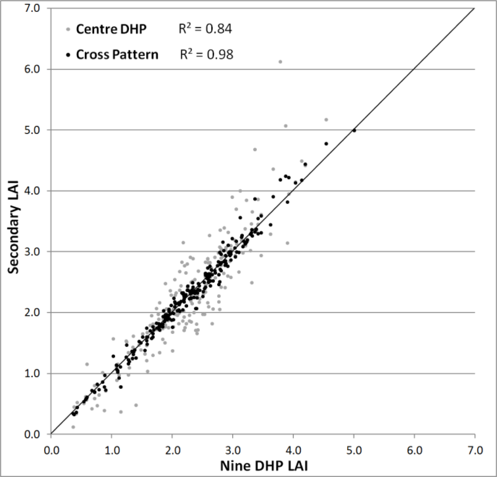
Using the regression model created with the calibration dataset to estimate values of LAI for the validation dataset resulted in the trend of predicted
versus in situ estimated values presented in
Figure 13. Scatter around the 1:1 line may be partially due to the time lag between the acquisition of the LiDAR data (
i.e., summer 2007) and
in situ data collection (
i.e., summer 2011). This phenomenon may have most affected younger plots, which had potential to gain most biomass and leaf area.
Existing work using LiDAR data alone to estimate LAI tends to show marginally better results than what was demonstrated here, but for different forest environments. A temperate coniferous forest study by Jensen
et al. [
15] was able to obtain an adjusted R
2 of 0.65 for their true LAI model and a slightly higher value (R
2 = 0.68) when examining LAI values without clumping index processing. Their final model also used four predictors:
i.e., crown closure above breast height, COVAR above breast height and two simple percentile variables. As their study had an even larger suite of predictor variables to draw from than this study it is significant that they also found utility in a low height crown closure and COVAR variable. The stronger explanatory power of the Jensen
et al. their model may be related to: (i) the different species in the temperate coniferous forest of Idaho, and/or (ii) the use of an LAI-2000 instead of DHP for
in situ LAI data collection.
Another coniferous study in the eastern United States showed even better results [
40]. This study compared
in situ LAI derived from the LAI-2000 to LiDAR metrics derived from high density LiDAR (
i.e., 5 m
−2) for intensively managed loblolly pine (
Pinus taeda L.) plantations. Results were presented for five models with an incrementally greater number of predictors; adjusted R
2 ranged from 0.61 with two predictors to 0.82 with six predictors. The comparable, four variable model to our study obtained an adjusted R
2 of 0.78 and used very different predictors,
i.e., mean (>1 m), P20 (>1 m), LPI (Laser penetration index − ground returns/(ground returns + all returns)) and mean intensity. This was one of the only studies we found that incorporated LiDAR intensity values alongside height and density metrics. High model explanatory power may have been linked to the single species (
i.e., plantation) nature of the study.
4.2. Spectral Vegetation Index Model
The results of this portion of the study were not entirely unexpected. A previous study by [
41] examined the relationships between DHP and optically (
i.e., MODIS) derived LAI across several different forest types. They found poor correlations for sites that had open canopies, branches extending to the ground surface, and relatively low LAI values, particularly in black and white spruce stands. Studies with conflicting results include Stenberg
et al. [
42] and Chen and Cihlar [
16], which use Landsat TM and ETM data, respectively. Stenberg
et al. [
42] found the NDVI/LAI correlation coefficient to be 0.55 in managed pine and spruce stands in Finland with LAI ranging from 0.36 to 3.72. One of the first to use NDVI to estimate LAI in boreal Canada, Chen and Cihlar [
16] obtained R
2’s of 0.50 and 0.42 for their two campaigns. LAI values ranged from 0.92 to 4.17.
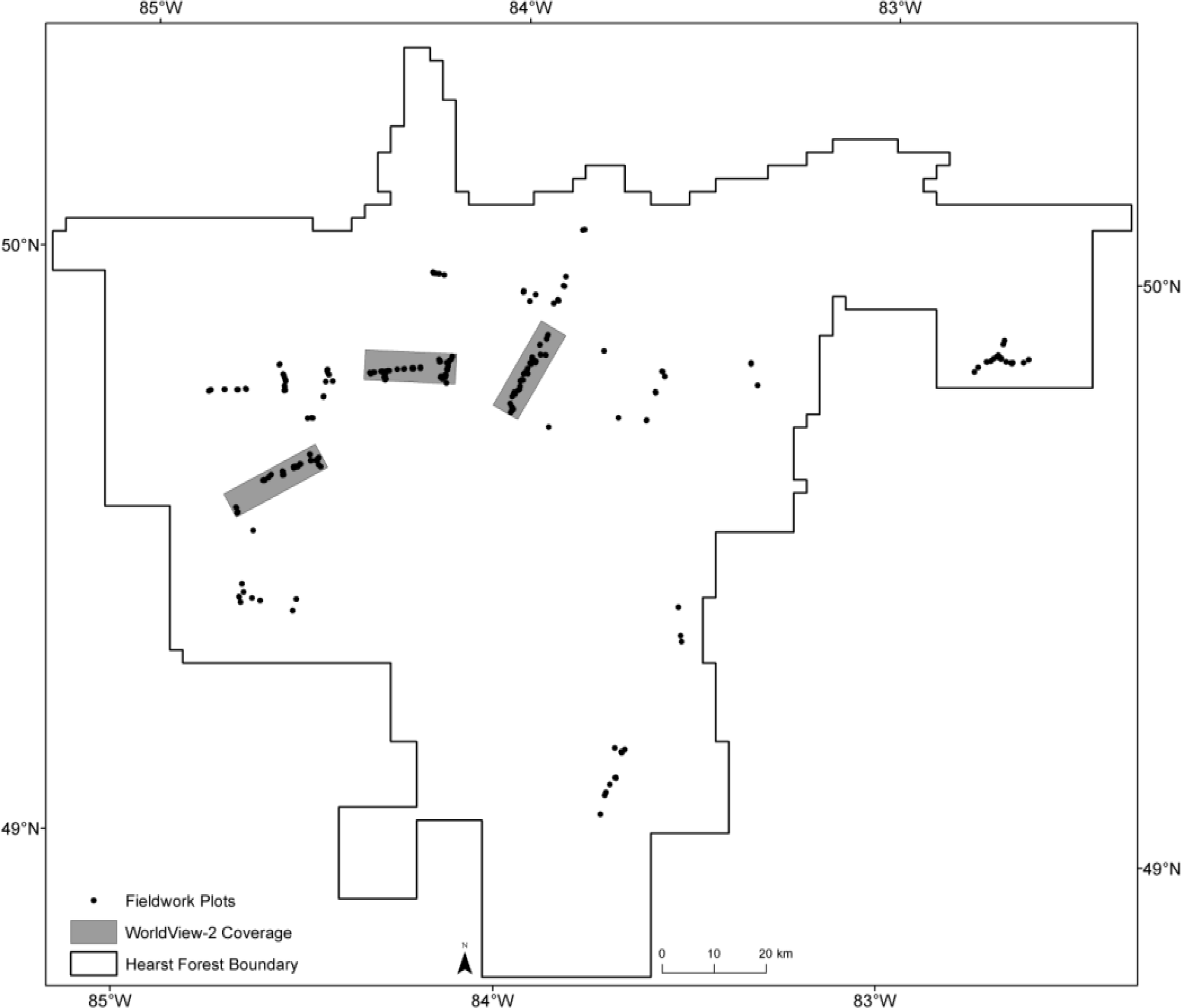
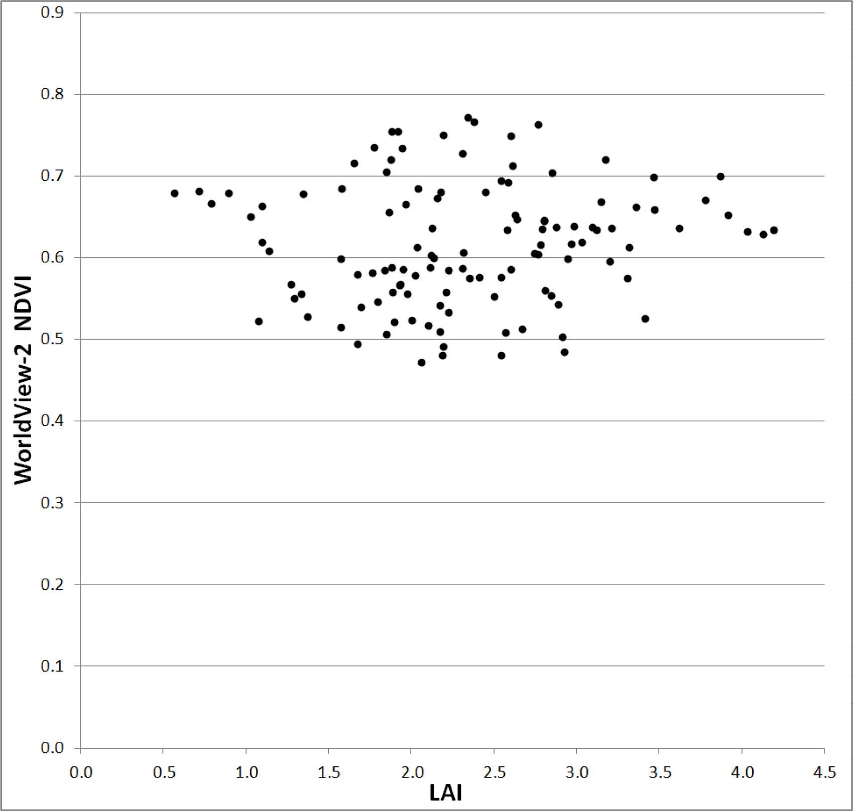
A Landsat-5 scene, acquired 14 August, 2008, was obtained for the same region as the WorldView-2 coverage and an NDVI surface was generated. The positive relationship between the two NDVI datasets was R2 = 0.61. A matched-pairs test of the WorldView-2 and Landsat values shows no statistical difference, with a null hypothesis-refuting p-value of 0.37. This relationship shows that the WorldView-2 NDVI values are comparable to the Landsat NDVI values.
It was originally surmised that the poor correlation was primarily due to a combination of the high spatial resolution of the sensor and the low spatial density of individual trees in the Hearst Forest (
i.e., open canopy), resulting in substantial shadowing and significant reflectance from the ground surface. Landsat-5 has significant, inherent averaging of reflectance, while Worldview-2 shows distinct tree crowns and gaps with associated shadows. While this phenomenon impacts measurements at the pixel level with WorldView-2 data, it is assumed that this is not the problem in this study. As was discussed earlier, for each plot the mean NDVI value was calculated, so the values being used for the WorldView-2 calculation include both crown and gap values, technically replicating the Landsat data, which integrates reflectance of each of these surfaces within the 30 m pixel. Even studies using lower spatial resolution sensors like AVHRR (
i.e., 1 km resolution) or MODIS (
i.e., 500 m resolution) obtained correlation coefficients between 0.39 and 0.46 [
17].
The most reasonable explanation for the poor performance of optical data in estimating LAI is due to the open canopies and the introduction of alternate understory spectra into the NDVI calculations. One of the failings of the DHP product was that it only provided an estimate of LAI from the focal point of the lens upwards,
i.e., 1.3 m. The cover below 1.3 m for the study sites ranged dramatically and included bare ground, thick moss and/or leafy shrubs, thereby impacting the NDVI values derived for these open canopy mixedwoods. As seen in several successful LiDAR studies, variables tend to be used that exclude this understory vegetation by implementing a height threshold of approximately one meter (e.g., [
14,
15,
40]).
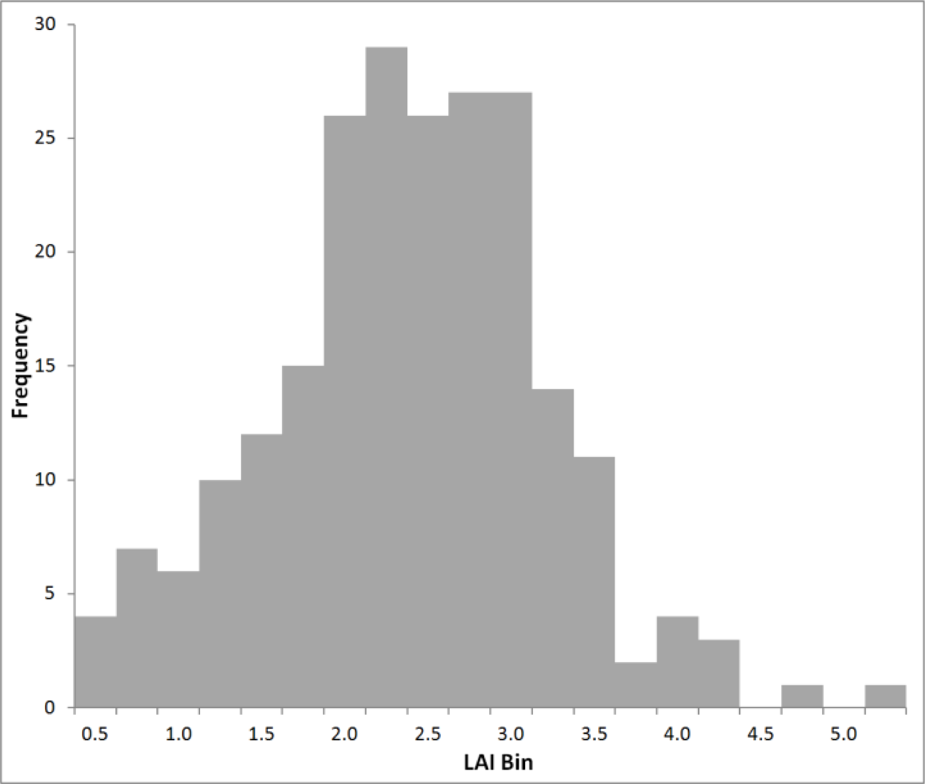
Deriving a statistical relationship was also difficult, given the narrow range of the NDVI and LAI values being compared. NDVI values ranged from 0.47 to 0.77 (range of 0.30) and LAI from 0.57 to 4.20 (range of 3.63). This range affected the ability of regression models to accurately depict trends in these data. Previously discussed successful models (e.g., [
43]) have ranges of LAI values as large as 0.2 to 8.5 and NDVI ranges from 0.6 to 0.93, and other studies have found that the wider ranges of other, non-normalized SVIs are better suited to LAI analysis [
42,
44]. As the plot sampling was specifically designed to sample both dense and relatively open areas, as judged by basal area measured the previous summer, this limited range is a product of the forest structure itself. The extensive single species dominance in some areas and physical similarity between several of the dominant tree species (e.g., trembling aspen/balsam poplar, white spruce/black spruce) generate similar canopy conditions in the boreal environment, exhibiting a low and narrow range of LAI.
4.3. Combination Model
It would seem that the addition of other LiDAR variables in conjunction with NDVI does not improve the models sufficiently to warrant further testing. This result was not unexpected considering the extremely poor correlation of NDVI values to LAI. While the model in
Equation (3) has the same explanatory power as the LiDAR-only model and a slightly lower RMSE%, the addition of a completely independent optical dataset is not financially feasible for operational implementation. One study that attempted a similar combinatorial approach using LiDAR variables integrated with SPOT-5 SVIs found an improvement from R
2 of 0.75 to 0.79 [
15]. This improvement to both explanatory power of the model and residual error (
i.e., 0.75 to 0.69) is small considering that the LiDAR-SPOT model used seven parameters, including two SVI (
i.e., reduced simple ratio and standard deviation of the red band), and the additional expense of acquiring a second remotely sensed dataset.
The results discussed here present a strong case for LiDAR modeling of LAI as opposed to more traditional optical approaches, particularly for the boreal mixedwood forests of central Ontario. Given the open canopies typical of the Hearst Forest, high resolution optical data tend to integrate surface spectra from all components of the plot (i.e., canopy, understory and ground) and for this region exhibit a narrow range of NDVI values. Conversely, LiDAR allows for a distinction between the forest canopy and the underlying ground cover, allowing it to better estimate LAI for the forest canopy alone.

