Processing and Assessment of Spectrometric, Stereoscopic Imagery Collected Using a Lightweight UAV Spectral Camera for Precision Agriculture

 ,
,
Abstract
:1. Introduction
2. A Method for Processing FPI Spectral Data Cubes
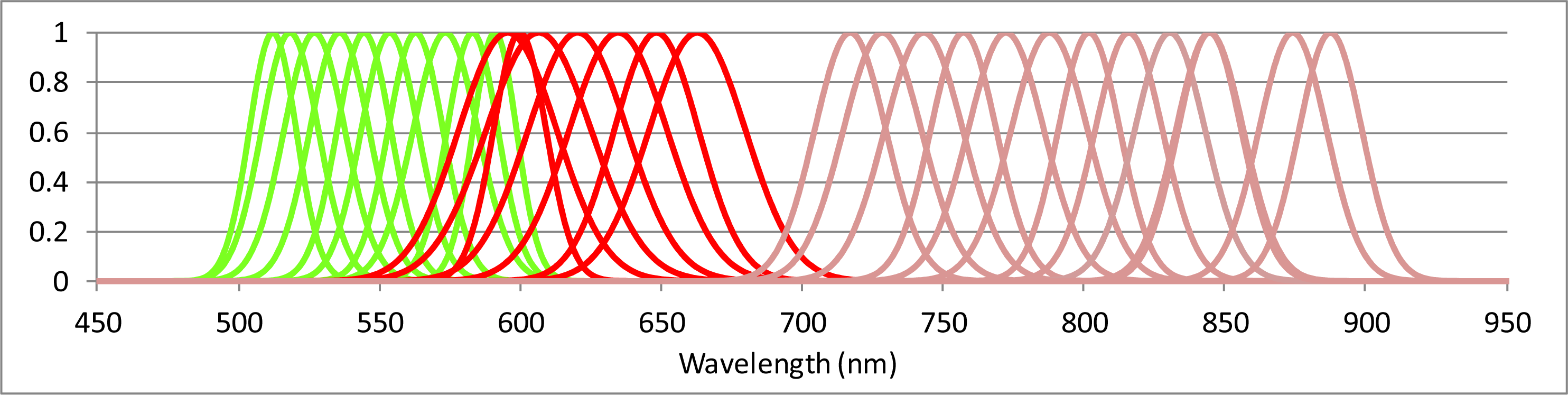
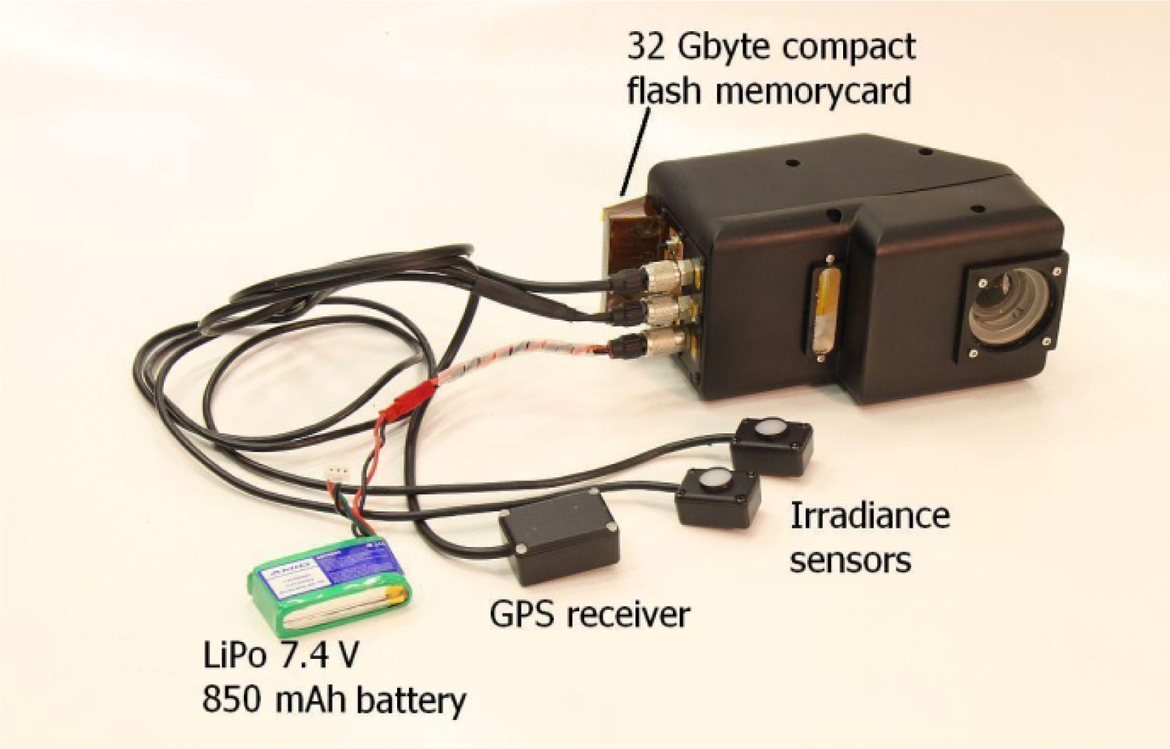
2.1. An FPI-Based Spectral Camera
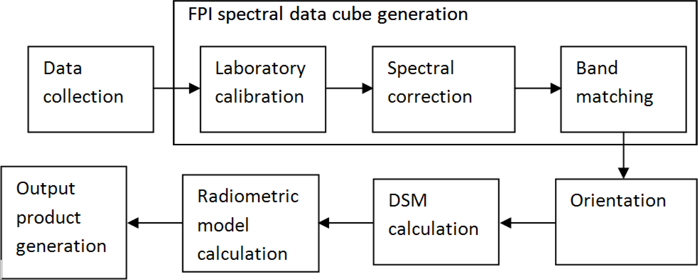
2.2. FPI Spectral Camera Data Processing
2.3. FPI Spectral Data Cube Generation
2.3.1. Radiometric Correction Based on Laboratory Calibration
2.3.2. Correction of the Spectral Smile
- Correcting images: Our assumption is that we can calculate smile-corrected images so that the corrected spectrums can be resampled from two spectrally (with a difference in peak wavelength preferably less than 10 nm) and temporally (with a spatial displacement less than 20 pixels) adjacent image bands.
- Using the central areas of the images: When images are collected with a minimum of 60% forward and side overlaps and when the most nadir parts of images are used, the smile effect is less than 5 nm and can be ignored in most applications (when the FWHM is 10–40 nm).
- Resampling a “super spectrum” for each object point of the overlapping images providing variable central wavelengths. The entire spectrum can be utilized in the applications.
2.3.3. Band Matching
- Determining the orientations of and georeferencing the individual bands separately. With this approach, there are number-of-bands (typically 20–48) image blocks that need to be processed. We used this approach in our investigation with the 2011 camera prototype, where we processed five bands [20,29].
- Sampling the bands of individual data cubes in relation to the geometry of a reference band. Orientations are determined for the image block with reference band images, and this orientation information is then applied to all other bands. We studied this approach for this investigation.
2.4. Radiometric Correction of Frame Image Block Data
3. Empirical Investigation
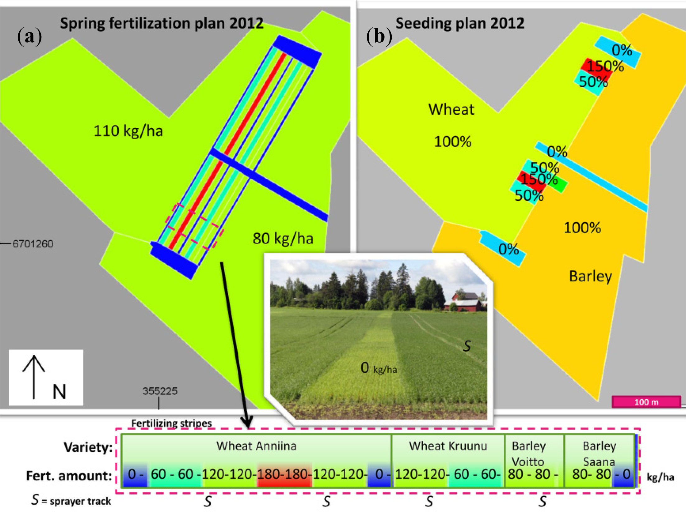
3.1. Test Area
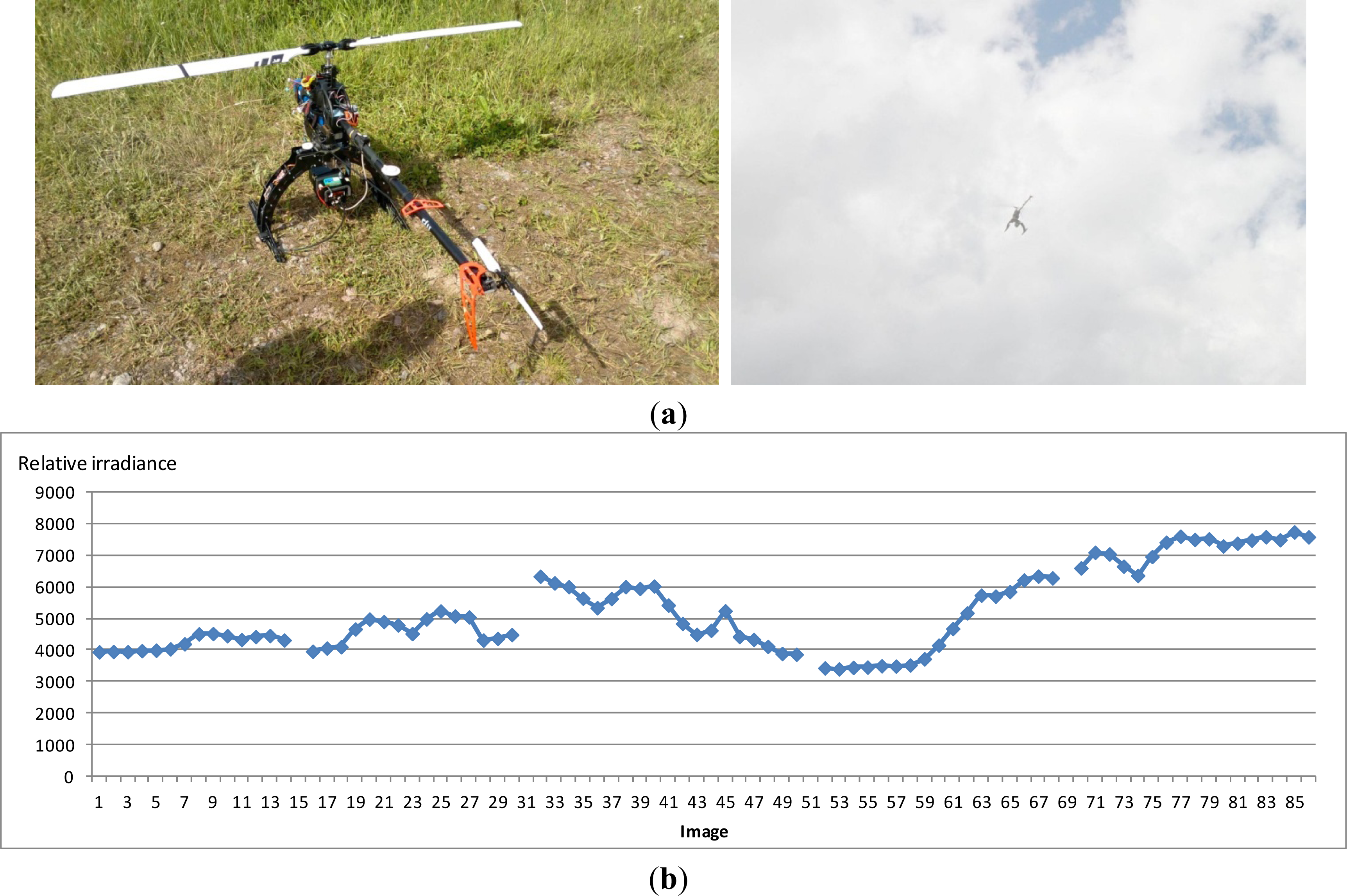
3.2. Flight Campaigns
3.3. Data Processing
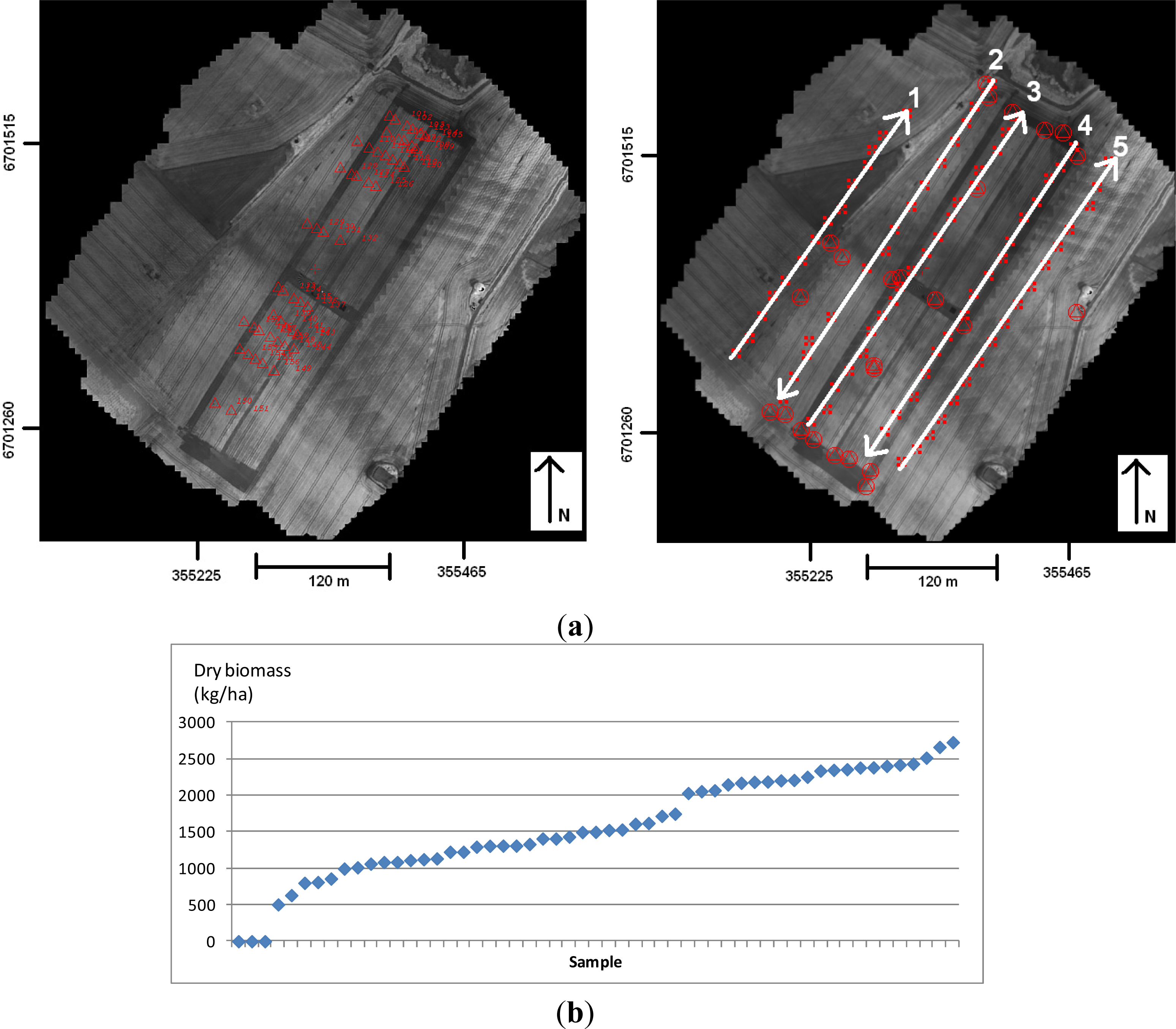
3.4. Biomass Estimation Using Spectrometric Data
4. Results
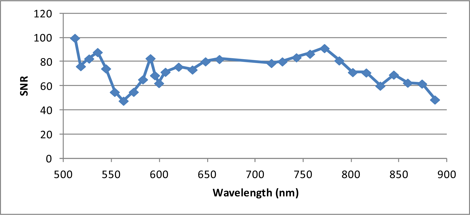
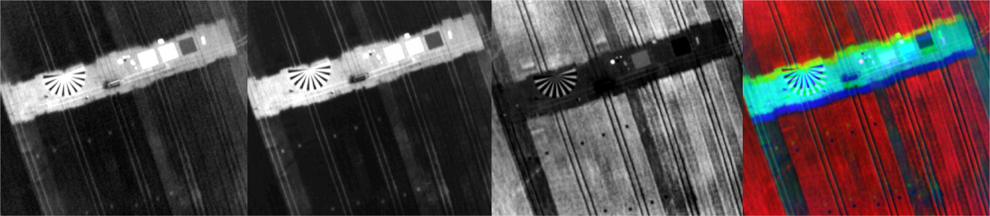
4.1. Image Quality
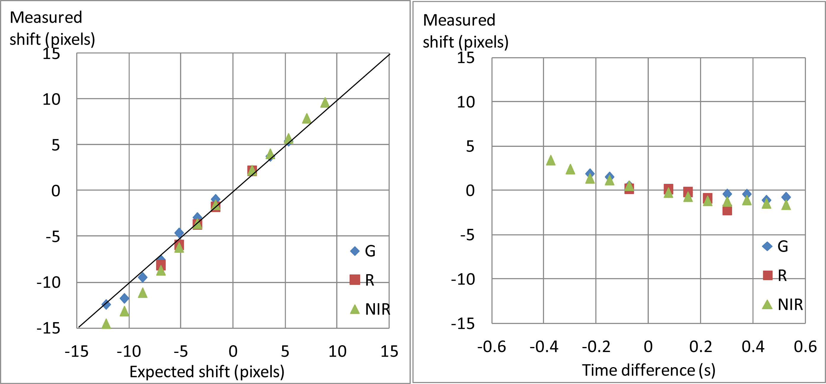
4.2. Band Matching
4.3. Geometric Processing
4.3.1. Orientations
4.3.2. DSM
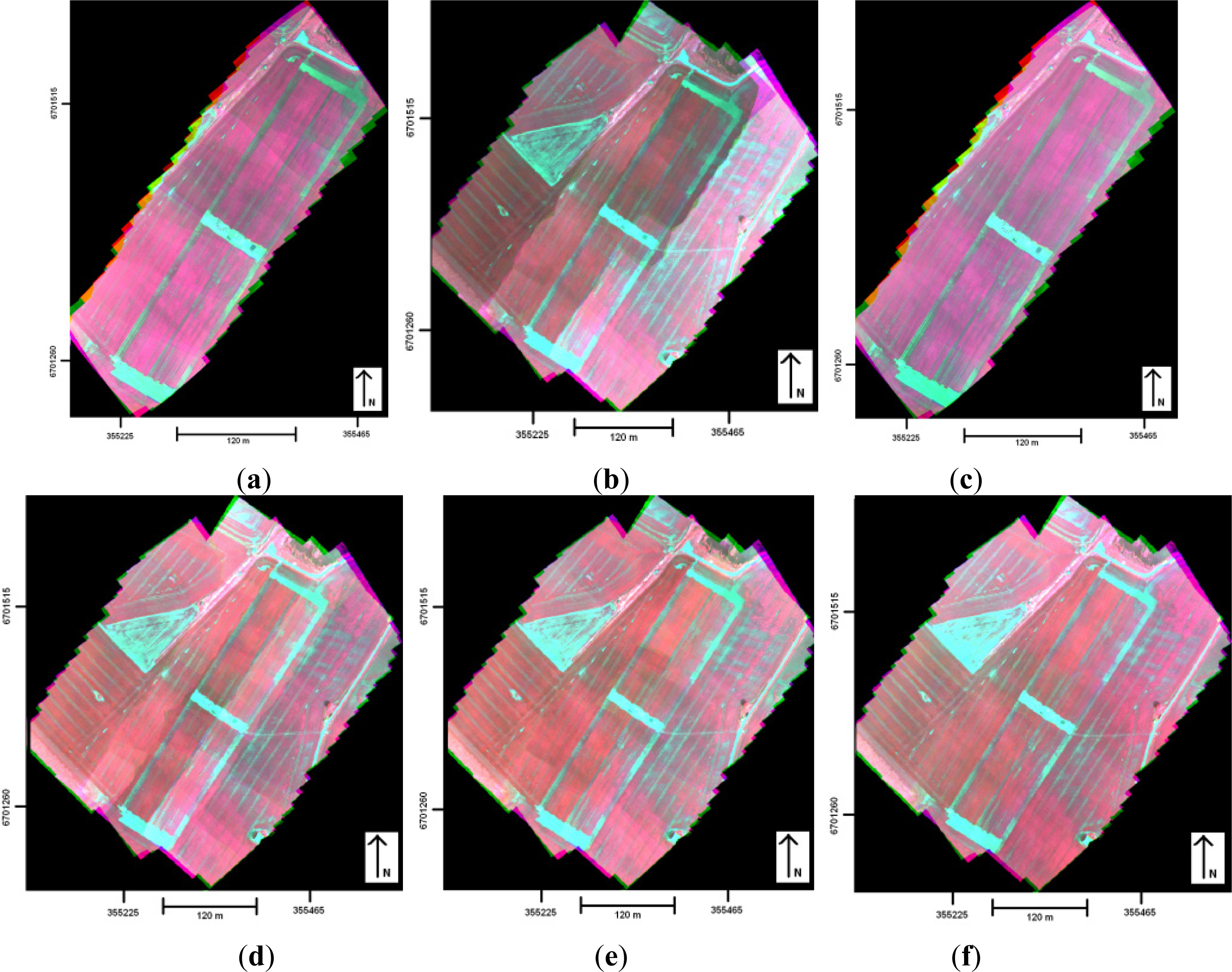
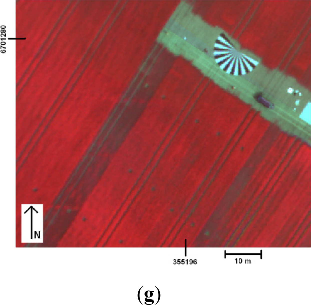
4.3.3. Image Mosaics
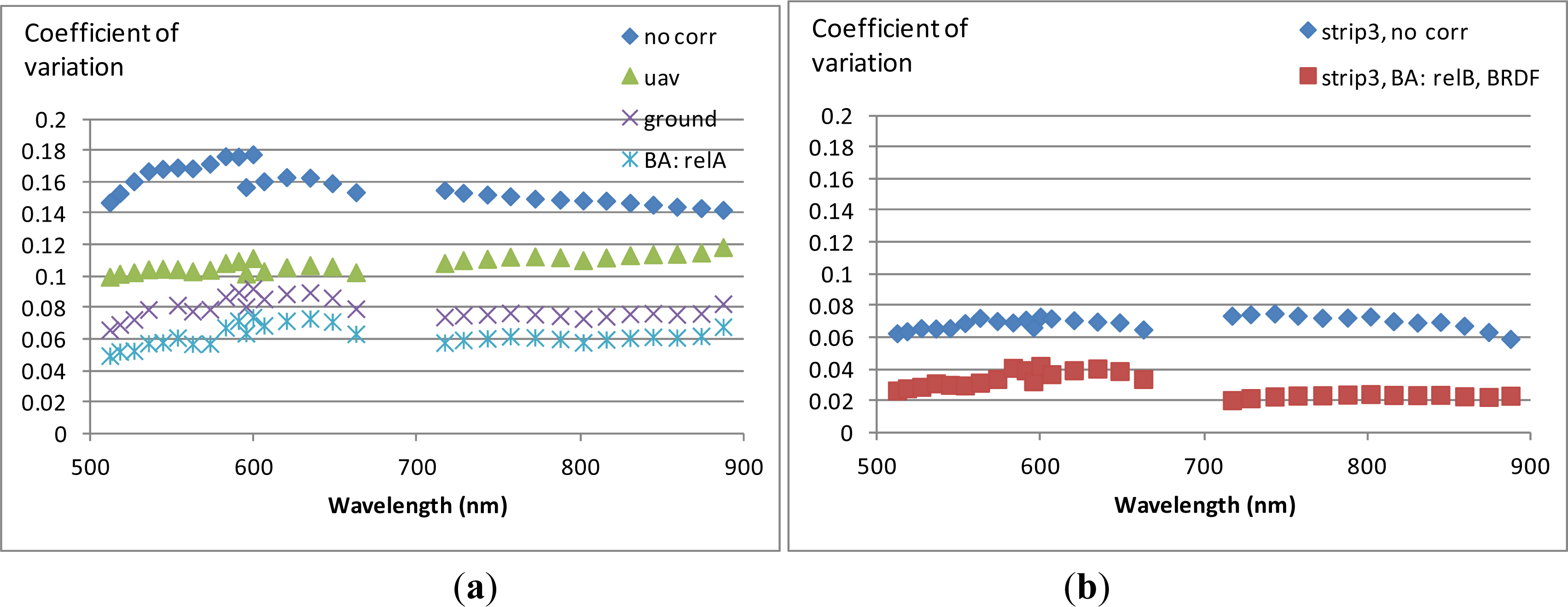
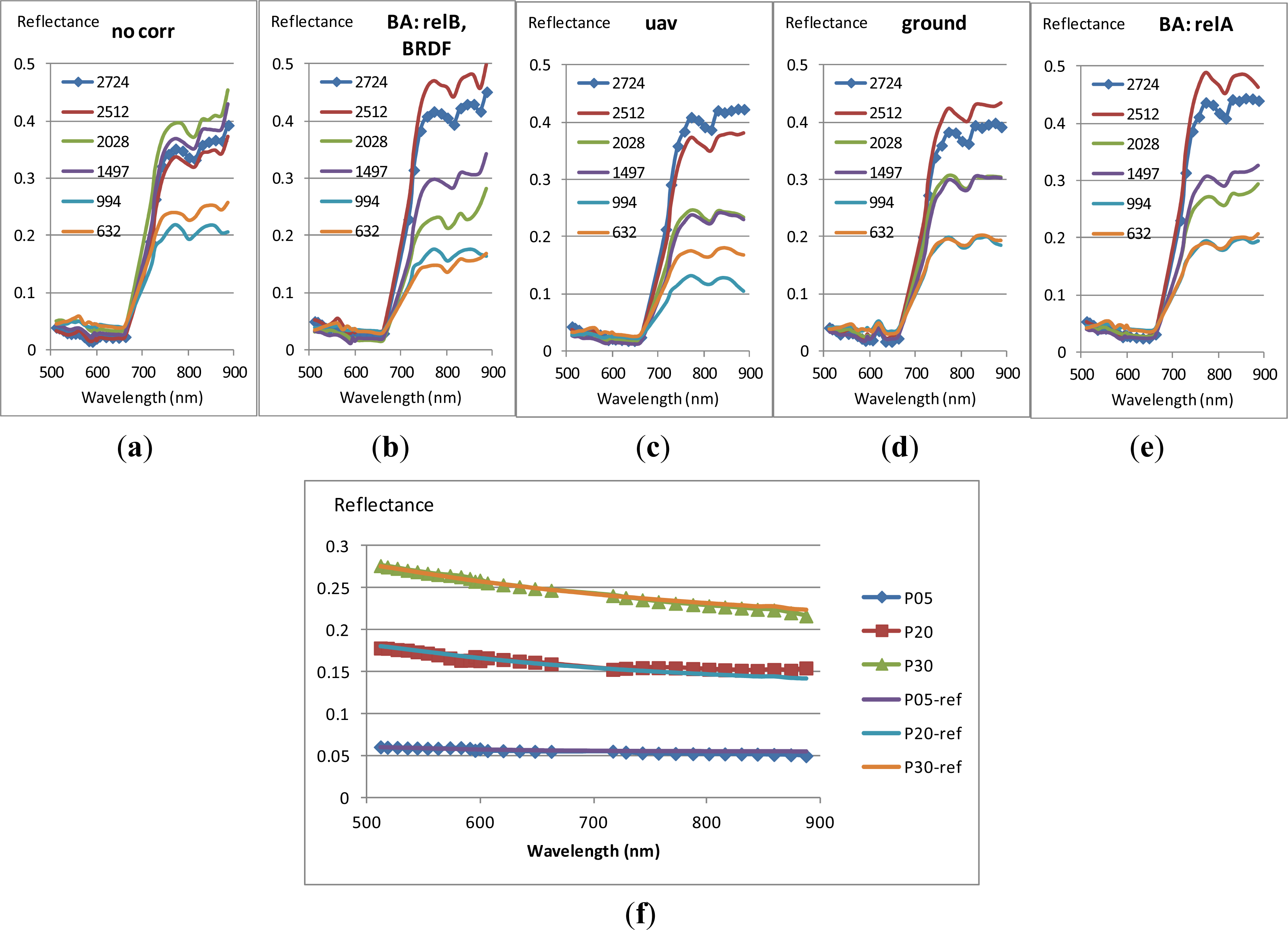
4.4. Radiometric Processing
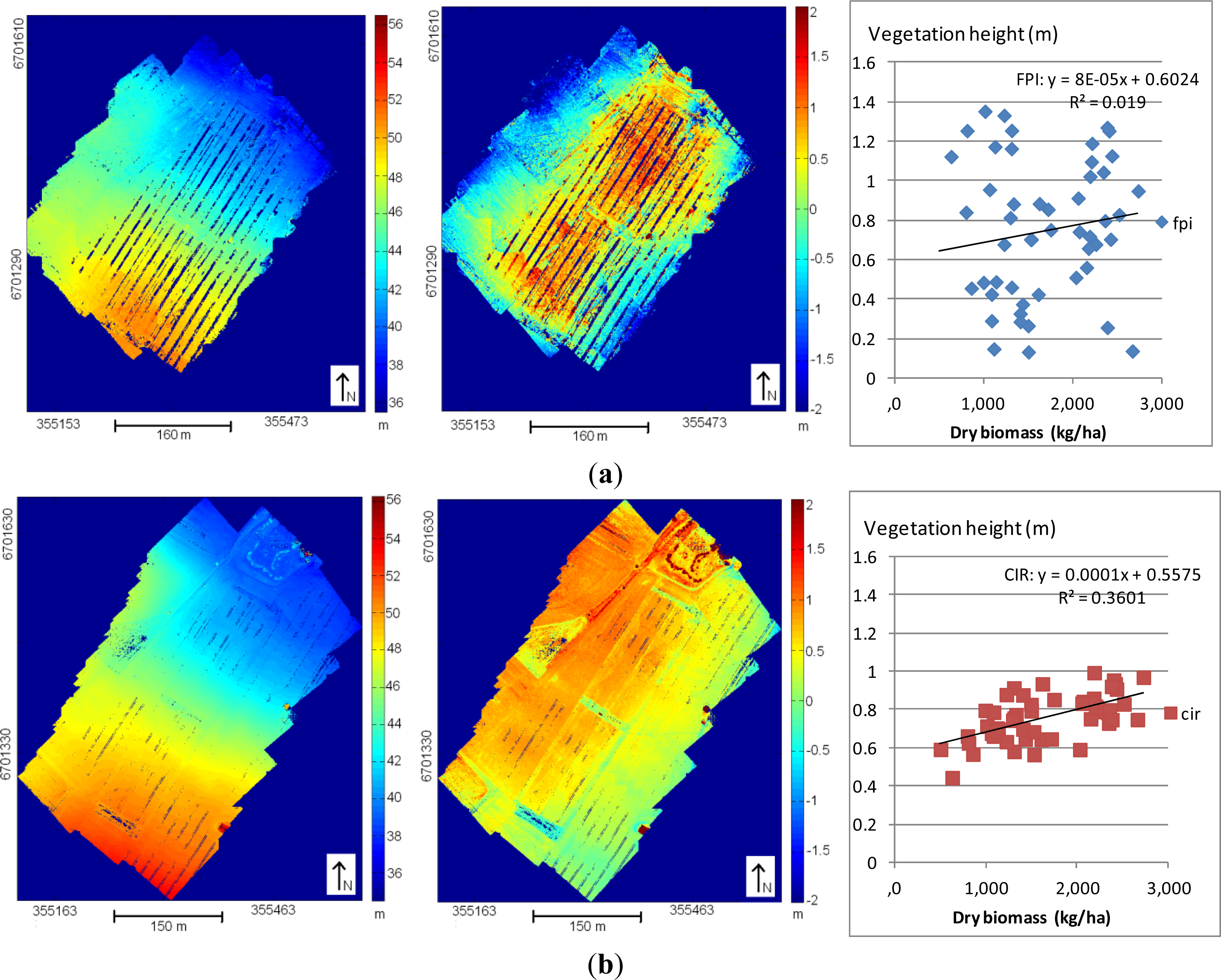
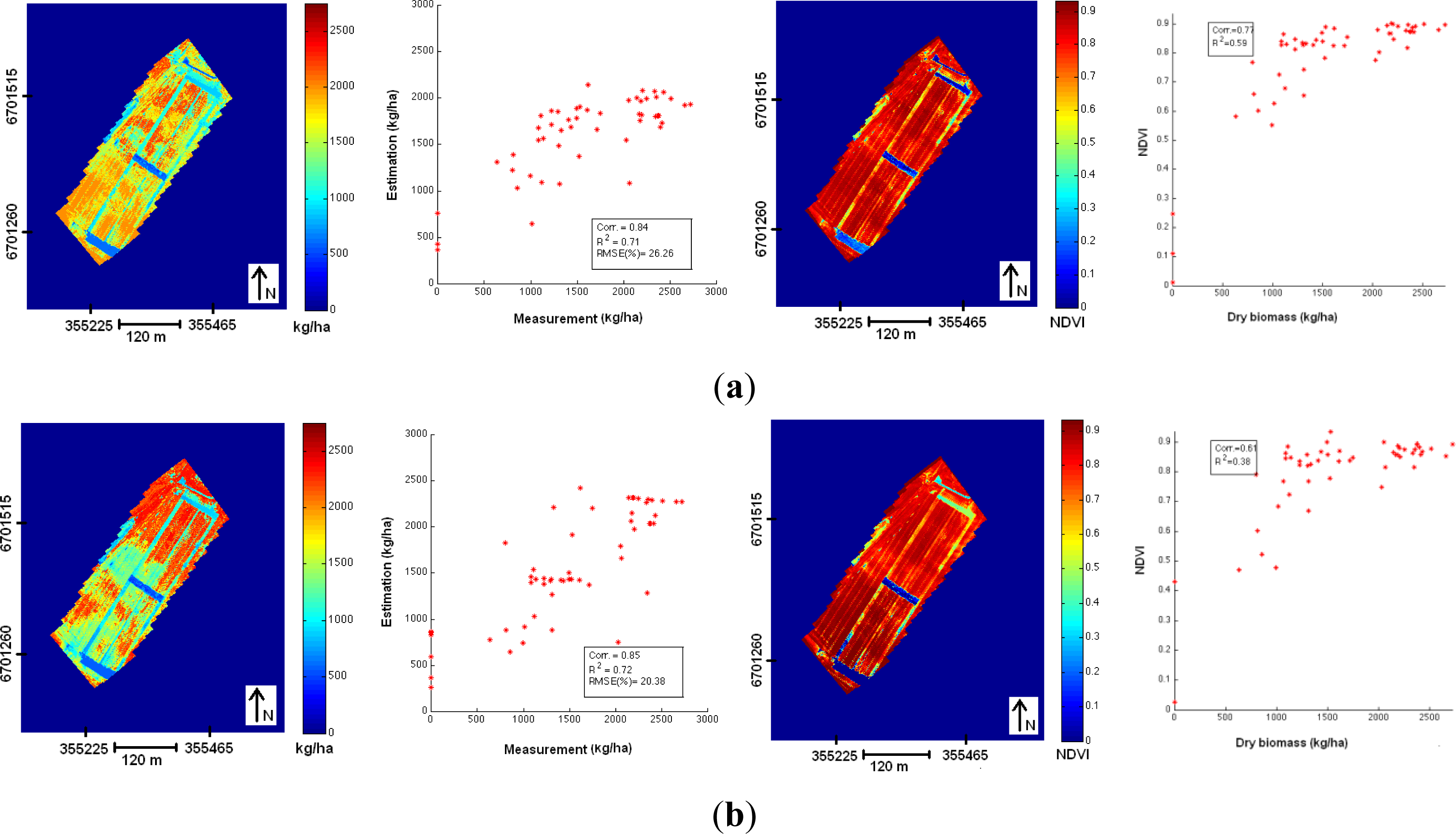
4.5. Biomass Estimation Using Spectrometric Information from the FPI Spectral Camera
5. Discussion
6. Conclusions
Acknowledgments
Conflict of Interest
References and Notes
- Hunt, E.R., Jr.; Hively, W.D.; Fujikawa, S.J.; Linden, D.S.; Daughtry, C.S.T.; McCarty, G.W. Acquisition of NIR-Green-Blue digital photographs from unmanned aircraft for crop monitoring. Remote Sens 2010, 2, 290–305. [Google Scholar]
- Lelong, C.C.D.; Burger, P.; Jubelin, G.; Roux, B.; Labbé, S.; Baret, F. Assessment of unmanned aerial vehicles imagery for quantitative monitoring of wheat crop in small plots. Sensors 2008, 8, 3557–3585. [Google Scholar]
- Zhou, G. Near real-time orthorectification and mosaic of small UAV video flow for time-critical event response. IEEE Trans. Geosci. Remote Sens 2009, 47, 739–747. [Google Scholar]
- Berni, J.A.; Zarco-Tejada, P.J.; Suárez, L.; Fereres, E. Thermal and narrowband multispectral remote sensing for vegetation monitoring from an unmanned aerial vehicle. IEEE Trans. Geosci. Remote Sens 2009, 47, 722–738. [Google Scholar]
- Laliberte, A.S.; Goforth, M.A.; Steele, C.M.; Rango, A. Multispectral remote sensing from unmanned aircraft: Image processing workflows and applications for rangeland environments. Remote Sens 2011, 3, 2529–2551. [Google Scholar]
- Saari, H.; Pellikka, I.; Pesonen, L.; Tuominen, S.; Heikkilä, J.; Holmlund, C.; Mäkynen, J.; Ojala, K.; Antila, T. Unmanned Aerial Vehicle (UAV) operated spectral camera system for forest and agriculture applications. Proc. SPIE 2011, 8174. [Google Scholar] [CrossRef]
- Hruska, R.; Mitchell, J.; Anderson, M.; Glenn, N.F. Radiometric and geometric analysis of hyperspectral imagery acquired from an unmanned aerial vehicle. Remote Sens 2012, 4, 2736–2752. [Google Scholar]
- Kelcey, J.; Lucieer, A. sensor correction of a 6-band multispectral imaging sensor for UAV remote sensing. Remote Sens 2012, 4, 1462–1493. [Google Scholar]
- Zarco-Tejada, P.J.; Gonzalez-Dugo, V.; Berni, J.A.J. Fluorescence, temperature and narrow-band indices acquired from a UAV platform for water stress using a micro-hyperspectral images and a thermal camera. Remote Sens. Environ 2012, 117, 322–337. [Google Scholar]
- Delauré, B.; Michiels, B.; Biesemans, J.; Livens, S.; Van Achteren, T. The Geospectral Camera: A Compact and Geometrically Precise Hyperspectral and High Spatial Resolution Imager. Proceedings of the ISPRS Hannover Workshop 2013, Hannover, Germany, 21–24 May 2013.
- Nagai, M.; Chen, T.; Shibasaki, R.; Kumgai, H.; Ahmed, A. UAV-borne 3-D mapping system by multisensory integration. IEEE Trans. Geosci. Remote Sens 2009, 47, 701–708. [Google Scholar]
- Jaakkola, A.; Hyyppä, J.; Kukko, A.; Yu, X.; Kaartinen, H.; Lehtomäki, M.; Lin, Y. A low-cost multi-sensoral mobile mapping system and its feasibility for tree measurements. ISPRS J. Photogramm. Remote Sens 2010, 65, 514–522. [Google Scholar]
- Wallace, L.; Lucieer, A.; Watson, C.; Turner, D. Development of a UAV-LiDAR system with application to forest inventory. Remote Sens 2012, 4, 1519–1543. [Google Scholar]
- Mäkynen, J.; Holmlund, C.; Saari, H.; Ojala, K.; Antila, T. Unmanned Aerial Vehicle (UAV) operated megapixel spectral camera. Proc. SPIE. [CrossRef]
- Alchanatis, V.; Cohen, Y. Spectral and Spatial Methods of Hyperspectral Image Analysis for Estimation of Biophysical and Biochemical Properties of Agricultural Crops. In Hyperspectral Remote Sensing of Vegetation, 1st ed; Thenkabail, P.S., Lyon, J.G., Huete, A., Eds.; CRC Press: Boca Raton, FL, USA, 2012; pp. 289–305. [Google Scholar]
- Zhang, C.; Kovacs, J.M. The application of small unmanned aerial systems for precision agriculture: a review. Precis. Agric 2012, 13, 693–712. [Google Scholar]
- Yao, H.; Tang, L.; Tian, L.; Brown, R.L.; Bhatngar, D.; Cleveland, T.E. Using Hyperspectral Data in Precision Farming Applications. In Hyperspectral Remote Sensing of Vegetation, 1st ed.; Thenkabail, P.S., Lyon, J.G., Huete, A., Eds.; CRC Press: Boca Raton, FL, USA, 2012; pp. 591–607. [Google Scholar]
- Zecha, C.W.; Link, J.; Claupein, W. Mobile sensor platforms: Categorisation and research applications in precision farming. J. Sens. Sens. Syst 2013, 2, 51–72. [Google Scholar]
- Nackaerts, K.; Delauré, B.; Everaerts, J.; Michiels, B.; Holmlund, C.; Mäkynen, J.; Saari, H. Evaluation of a lightweigth UAS-prototype for hyperspectral imaging. Int. Arch. Photogramm. Remote Sens. Spat. Infor. Sci 2010, 38, 478–483. [Google Scholar]
- Honkavaara, E.; Kaivosoja, J.; Mäkynen, J.; Pellikka, I.; Pesonen, L.; Saari, H.; Salo, H.; Hakala, T.; Markelin, L.; Rosnell, T. Hyperspectral reflectance signatures and point clouds for precision agriculture by light weight UAV imaging system. ISPRS Annal. Photogramm. Remote Sens. Spat. Inf. Sci 2012, I-7, 353–358. [Google Scholar]
- Pölönen, I.; Salo, H.; Saari, H.; Kaivosoja, J.; Pesonen, L.; Honkavaara, E. Biomass estimator for NIR image with a few additional spectral band images taken from light UAS. Proc. SPIE 2012(8369). [CrossRef]
- Scholten, F.; Wewel, F. Digital 3D-data acquisition with the high resolution stereo camera-airborne (HRSC-A). Int. Arch. Photogramm. Remote Sens. Spat. Infor. Sci 2000, 33, 901–908. [Google Scholar]
- Leberl, F.; Irschara, A.; Pock, T.; Meixner, P.; Gruber, M.; Scholz, S.; Wiechert, A. Point clouds: Lidar versus 3D vision. Photogramm. Eng. Remote Sens 2010, 76, 1123–1134. [Google Scholar]
- Haala, N.; Hastedt, H.; Wolf, K.; Ressl, C.; Baltrusch, S. Digital photogrammetric camera evaluation—Generation of digital elevation models. Photogramm. Fernerkund. Geoinf 2010, 2, 99–115. [Google Scholar]
- Hirschmüller, H. Semi-Global Matching: Motivation, Development and Applications. In Photogrammetric Week 2011; Fritsch, D., Ed.; Wichmann Verlag: Heidelberg, Germany, 2011; pp. 173–184. [Google Scholar]
- Rosnell, T.; Honkavaara, E. Point cloud generation from aerial image data acquired by a quadrocopter type micro unmanned aerial vehicle and a digital still camera. Sensors 2012, 12, 453–480. [Google Scholar]
- Rosnell, T.; Honkavaara, E.; Nurminen, K. On geometric processing of multi-temproal image data collected by light UAV systems. Int. Arch. Photogramm. Remote Sens. Spat. Infor. Sci 2011, 38, 63–68. [Google Scholar]
- Schaepman-Strub, G.; Schaepman, M.E.; Painter, T.H.; Dangel, S.; Martonchik, J.V. Reflectance quantities in optical remote sensing—Definitions and case studies. Remote Sen. Environ 2006, 103, 27–42. [Google Scholar]
- Honkavara, E.; Hakala, T.; Saari, H.; Markelin, L.; Mäkynen, J.; Rosnell, T. A process for radiometric correction of UAV image blocks. Photogramm. Fernerkund. Geoinfor 2012. [Google Scholar] [CrossRef]
- Förstner, W.; Gülch, E. A Fast Operator for Detection and Precise Location of Distinct Points, Corners and Centers of Circular Features. Proceedings of Intercommission Conference on Fast Processing of Photogrammetric Data, Interlaken, Swizerland, 2–4 June 1987; pp. 281–305.
- Beisl, U. New Method for Correction of Bidirectional Effects in Hyperspectral Images. Proceedings of Remote Sensing for Environmental Monitoring, GIS Applications, and Geology, Toulouse, France, 17 September 2001.
- Walthall, C.L.; Norman, J.M.; Welles, J.M.; Campbell, G.; Blad, B.L. Simple equation to approximate the bidirectional reflectance from vegetative canopies and bare soil surfaces. Appl. Opt 1985, 24, 383–387. [Google Scholar]
- Hakala, T.; Honkavaara, E.; Saari, H.; Mäkynen, J.; Kaivosoja, J.; Pesonen, L.; Pölönen, I. Spectral imaging from UAVs under varying illumination conditions. Int. Arch. Photogramm. Remote Sens. Spat. Infor. Sci. 2013, XL-1/W2, 189–194. [Google Scholar]
- Kuvatekniikka Oy Patrik Raski. Available online: http://kuvatekniikka.com/ (accessed on 5 September 2013).
- Intersil ISL29004 Datasheet. Available online: http://www.intersil.com/content/dam/Intersil/documents/fn62/fn6221.pdf (accessed on 9 October 2013).
- Kotsiantis, S.B. Supervised machine learning: A review of classification techniques. Informatica 2007, 31, 249–268. [Google Scholar]
- National Land Survey of Finland Open Data License. Available on line: http://www.maanmittauslaitos.fi/en/NLS_open_data_licence_version1_20120501 (accessed on 10 October 2013).
- Chiang, K.-W.; Tsai, M.-L.; Chu, C.-H. The development of an UAV borne direct georeferenced photogrammetric platform for ground control point free applications. Sensors 2012, 12, 9161–9180. [Google Scholar]
- Turner, D.; Lucieer, A.; Watson, C. An automated technique for generating georectified mosaics from ultra-high resolution Unmanned Aerial Vehicle (UAV) imagery, based on Structure from Motion (SfM) point clouds. Remote Sens 2012, 4, 1392–1410. [Google Scholar]
- Snavely, N. Bundler: Structure from Motion (SFM) for Unordered Image Collections. Available online: phototour.cs.washington.edu/bundler/ (accessed on 12 July 2013).
- Mathews, A.J.; Jensen, J.L.R. Visualizing and quantifying vineyard canopy LAI using an Unmanned Aerial Vehicle (UAV) collected high density structure from motion point cloud. Remote Sens 2013, 5, 2164–2183. [Google Scholar]
- Honkavaara, E.; Arbiol, R.; Markelin, L.; Martinez, L.; Cramer, M.; Bovet, S.; Chandelier, L.; Ilves, R.; Klonus, S.; Marshal, P.; et al. Digital airborne photogrammetry—A new tool for quantitative remote sensing?—A state-of-the-Art review on radiometric aspects of digital photogrammetric images. Remote Sens 2009, 1, 577–605. [Google Scholar]
- Richter, R.; Schläpfer, D. Geo-atmospheric processing of airborne imaging spectrometry data. Part 2: Atmospheric/topographic correction. Int. J. Remote Sens 2002, 23, 2631–2649. [Google Scholar]
- Richter, R.; Kellenberger, T.; Kaufmann, H. Comparison of topographic correction methods. Remote Sens 2009, 1, 184–196. [Google Scholar]
- Beisl, U.; Telaar, J.; von Schönemark, M. Atmospheric Correction, Reflectance Calibration and BRDF Correction for ADS40 Image Data. Proceedings of the XXI ISPRS Congress, Commission VII, Beijing, China, 3–11 July 2008.
- Chandelier, L.; Martinoty, G. Radiometric aerial triangulation for the equalization of digital aerial images and orthoimages. Photogramm. Eng. Remote Sens 2009, 75, 193–200. [Google Scholar]
- Collings, S.; Cacetta, P.; Campbell, N.; Wu, X. Empirical models for radiometric calibration of digital aerial frame mosaics. IEEE Trans. Geosci. and Remote Sens 2011, 49, 2573–2588. [Google Scholar]
- López, D.H.; García, B.F.; Piqueras, J.G.; Aöcázar, G.V. An approach to the radiometric aerotriangulation of photogrammetric images. ISPRS J. Photogramm. Remote Sens 2011, 66, 883–893. [Google Scholar]
- Atzberger, C. Advances in remote sensing of agriculture: Context description, existing operational monitoring systems and major information needs. Remote Sens 2013, 5, 949–981. [Google Scholar]
- Watts, A.C.; Ambrosia, V.G.; Hinkley, E.A. Unmanned Aircraft Systems in remote sensing and scientific research: Classification and considerations of use. Remote Sens 2012, 4, 1671–1692. [Google Scholar]


| Parameter | Prototype 2011 | Prototype 2012 |
|---|---|---|
| Horizontal and vertical FOV (°) | >36, >26 | >50, >37 |
| Nominal focal length (mm) | 9.3 | 10.9 |
| Wavelength range (nm) | 400–900 | 400–900 |
| Spectral resolution at FWHM (nm); depending on the selection of the FPI air gap value | 9–45 | 10–40 |
| Spectral step (nm): adjustable by controlling the air gap of the FPI | <1 | <1 |
| f-number | <7 | <3 |
| Pixel size (μm); no binning/default binning | 2.2/8.8 | 5.5/11 |
| Maximum spectral image size (pixels) | 2,592 × 1,944 | 2,048 × 2,048 |
| Spectral image size with default binning (pixels) | 640 × 480 | 1,024 × 648 |
| Camera dimensions (mm) | 65 × 65 × 130 | <80 × 92 × 150 |
| Weight (g); including battery, GPS receiver, downwelling irradiance sensors and cabling | <420 | <700 |
| Raw Data, 42 Bands |
| Central peak wavelength (nm): 506.8, 507.4, 507.9, 508.4, 510.2, 515.4, 523.3, 533.0, 541.3, 544.1, 550.5, 559.6, 569.7, 581.3, 588.6, 591.3, 596.7, 601.7, 606.7, 613.8, 629.5, 643.1, 649.7, 657.2, 672.6, 687.3, 703.2, 715.7, 722.7, 738.8, 752.7, 766.9, 783.2, 798.1, 809.5, 811.1, 826.4, 840.6, 855.2, 869.9, 884.5, 895.4 |
| FWHM (nm): 14.7, 22.1, 15.2, 16.7, 19.7, 23.8, 25.5, 24.9, 22.7, 12.7, 23.9, 23.0, 27.2, 21.4, 18.3, 41.1, 22.1, 44.0, 21.4, 41.5, 41.1, 35.3, 12.9, 40.4, 36.5, 38.3, 33.5, 29.9, 32.7, 32.8, 27.6, 31.8, 32.1, 25.9, 14.7, 28.2, 29.5, 26.5, 28.3, 28.4, 26.4, 22.3 |
| Smile Corrected Data, 30 Bands |
| Central peak wavelength (nm): 511.8, 517.9, 526.6, 535.5, 544.2, 553.3, 562.5, 573.1, 582.7, 590.6, 595.2, 599.5, 606.2, 620.0, 634.4, 648.0, 662.5, 716.8, 728.2, 742.9, 757.0, 772.1, 787.5, 801.6, 815.7, 830.3, 844.4, 859.0, 873.9, 887.3 |
| FWHM (nm): 19.7, 23.8, 25.5, 24.9, 22.7, 23.9, 23.0, 27.2, 21.4, 18.3, 41.1, 22.1, 44.0, 41.5, 41.1, 35.3, 40.4, 29.9, 32.7, 32.8, 27.6, 31.8, 32.1, 25.9, 28.2, 29.5, 26.5, 28.3, 28.4, 26.4 |
| Calculation Case (id) | Dataset | Parameters |
|---|---|---|
| No correction (no corr) | Full, Strip 3 | aabs, babs |
| Relative radiometric correction using wide-bandwidth irradiance measured in UAV (uav) | Full | Cj, aabs, babs |
| Relative radiometric correction using spectral irradiance measured on the ground (ground) | Full | Cj(λ), aabs, babs |
| Radiometric block adjustment with relative multiplicative correction (BA: relA) | Full | arel_j, aabs, babs |
| Radiometric block adjustment with BRDF and relative additive correction (BA: relB, BRDF) | Strip 3 | brel_j, a’, b’, aabs, babs |
| Band | σ0 | RMSE Positions (m) | RMSE Rotations (°) | RMSE GCPs (m) | N | ||||||
|---|---|---|---|---|---|---|---|---|---|---|---|
| (pixels) | X0 | Y0 | Z0 | ω | φ | κ | X | Y | Z | ||
| 7 | 0.68 | 0.28 | 0.27 | 0.06 | 0.105 | 0.107 | 0.019 | 0.08 | 0.10 | 0.05 | 9,10 |
| 16 | 0.73 | 0.26 | 0.25 | 0.06 | 0.094 | 0.100 | 0.018 | 0.06 | 0.13 | 0.05 | 11,13 |
| 29 | 0.49 | 0.24 | 0.24 | 0.06 | 0.091 | 0.093 | 0.016 | 0.14 | 0.13 | 0.03 | 10,13 |
| Band | Parameters | Standard Deviation | ||||
|---|---|---|---|---|---|---|
| x0 (mm) | y0 (mm) | k1 (mm·mm−3) | x0 (mm) | y0 (mm) | k1 (mm·mm−3) | |
| 7 | 0.270 | −0.023 | 0.00251 | 0.003 | 0.006 | 1.26E-05 |
| 16 | 0.242 | −0.091 | 0.00252 | 0.002 | 0.005 | 1.07E-05 |
| 29 | 0.208 | −0.132 | 0.00251 | 0.002 | 0.005 | 1.06E-05 |
© 2013 by the authors; licensee MDPI, Basel, Switzerland This article is an open access article distributed under the terms and conditions of the Creative Commons Attribution license ( http://creativecommons.org/licenses/by/3.0/).
Share and Cite
Honkavaara, E.; Saari, H.; Kaivosoja, J.; Pölönen, I.; Hakala, T.; Litkey, P.; Mäkynen, J.; Pesonen, L. Processing and Assessment of Spectrometric, Stereoscopic Imagery Collected Using a Lightweight UAV Spectral Camera for Precision Agriculture. Remote Sens. 2013, 5, 5006-5039. https://doi.org/10.3390/rs5105006
Honkavaara E, Saari H, Kaivosoja J, Pölönen I, Hakala T, Litkey P, Mäkynen J, Pesonen L. Processing and Assessment of Spectrometric, Stereoscopic Imagery Collected Using a Lightweight UAV Spectral Camera for Precision Agriculture. Remote Sensing. 2013; 5(10):5006-5039. https://doi.org/10.3390/rs5105006
Chicago/Turabian StyleHonkavaara, Eija, Heikki Saari, Jere Kaivosoja, Ilkka Pölönen, Teemu Hakala, Paula Litkey, Jussi Mäkynen, and Liisa Pesonen. 2013. "Processing and Assessment of Spectrometric, Stereoscopic Imagery Collected Using a Lightweight UAV Spectral Camera for Precision Agriculture" Remote Sensing 5, no. 10: 5006-5039. https://doi.org/10.3390/rs5105006
APA StyleHonkavaara, E., Saari, H., Kaivosoja, J., Pölönen, I., Hakala, T., Litkey, P., Mäkynen, J., & Pesonen, L. (2013). Processing and Assessment of Spectrometric, Stereoscopic Imagery Collected Using a Lightweight UAV Spectral Camera for Precision Agriculture. Remote Sensing, 5(10), 5006-5039. https://doi.org/10.3390/rs5105006