1. Introduction
Soil moisture content (SMC), along with its temporal and spatial distribution, is widely considered as a key variable in numerous environmental disciplines, especially in climatology, meteorology, hydrology and agriculture. For hydrological and agricultural purposes, the SMC plays a fundamental role, since it controls the water available for vegetation growth [
1,
2], as well as the recharge of deep aquifers [
3]. In meteorology, the SMC has a great impact on the energy transfer from surface into atmosphere by regulating the evapotranspiration [
4]. Moreover, a timely and precise SMC knowledge has a significant impact in various risk management applications, such as drought and flooding prediction and management [
5].
Due to high variability of SMC in time and space, proper estimation of this variable is quite challenging. Ground measurements and remote sensing methods can be considered powerful tools for the SMC quantification. Ground measurements, such as those obtained by using calibrated probes (e.g., those based on Time Domain Reflectometry (TDR) techniques), can provide reliable point-scale measurements and, in case of distributed sensors, can also help in understanding the soil moisture patterns across-scales [
6,
7]. However, when the catchment or basin scale is considered, the information needs to be spatially distributed and, in this case, ground measurements are not suitable, since their extension to a larger scale is very expensive and time-consuming, thus not being affordable from an economic and manpower point of view. On the other hand, microwave remote sensing techniques can allow detecting SMC at a basin scale.
Remote sensing from active (SAR and scatterometer) and passive sensors (radiometers) have demonstrated to be good and flexible tools to detect spatial and temporal SMC [
8–
13].
Regarding the spatial resolution, the SMC estimates from microwave remote sensing can span from tens of meters up to 50 km, whereas, the highest temporal resolution can be achieved with monthly or bimonthly acquisitions. Low spatial resolution estimates can be instead available worldwide on a daily basis. Upcoming sensors such as Sentinel 1 and SMAP will represent a further step to overcome these limitations. Sentinel 1 will work at C-band with a rather high spatial resolution of 5 m × 20 m and the temporal repetition frequency of 5–6 days over the European continent and 12 days for global acquisitions. Moreover, recent studies based on Sentinel 1-like data indicated that the improved radiometric resolution of Sentinel 1 may also produce a reduction in the retrieval errors on SMC [
14].
It is also worthwhile mentioning the NASA Soil Moisture Active Passive (SMAP) mission that will offer the uniqueness of radar and radiometric simultaneous observations at L-band, with a ground resolution of around 1 km and a temporal resolution of 3 days [
15].
It should be noted that all microwave sensors are able to estimate SMC referring to the first few centimeters of soil only. One proposed solution to improve the spatial and temporal resolution of available SMC information and to simulate SMC for deeper soil layers is related to the assimilation of SMC, derived from remote sensing data, into hydrological and land surface models [
5,
16]. The main aim of this procedure would be to update and/or calibrate intermediate or final states of the model variables; thus, obtaining an improved estimation of water discharge and/or atmospheric drivers, as a major output. Notable improvements have been made in the model assimilation scheme, especially in view of assimilating long-time series of SMC estimates. Reichle and Koster [
17] assimilated the Global Soil Moisture Data Bank into NASA catchment land surface model, reaching an improvement in the annual cycle of surface and root zone SMC in comparison with ground data. Also the temporal behavior showed reduced but significant improvement in the correlation with ground measurements.
Crow and Ryu [
18] proposed a new algorithm to improve the forecast of run-off through the assimilation of soil moisture values in a sequential way. The work demonstrated that the assimilation can improve the retrieval of both pre-storm soil moisture conditions and storm-scale rainfall accumulations.
Draper
et al. [
19] have focused their work on the assimilation of available data sets from passive (AMSR-E) and active (ASCAT) sensors into the NASA catchment land surface model. The impact of assimilating each dataset on the modeled soil moisture skill was evaluated using in-situ soil moisture observations in the SCAN/SNOTEL network in the US and the Murrumbidgee Soil Moisture Monitoring Network in southeast Australia. Their research demonstrated that the combined used of SMC estimates from active and passive sensors produced an increase in the retrieval accuracy for each land cover class, with significant improvements for both root-zone and surface soil moisture over croplands, grasslands, and mixed cover.
A necessary step before data assimilation is the comparison between SMC estimated by models and by remote sensing data, in order to verify the compatibility between these two sources of information [
16–
20]. This step is essential to better understand if the back-propagated SMC simulated by the model can be then compatible with remote sensing estimates. Moreover, at local scale, some differences due to human interventions need to be properly evaluated in both model and remote sensing estimates, such as the presence of tillage activities. In this view, in fact, Pellenq [
21] indicated that it is essential to accurately understand all the processes involved in the soil moisture variability as well as their scale interactions. In the study of Mattia [
22], hydrological models were used to provide a-priori information in the retrieval process of SMC from remotely sensed data to help disentangling the effect of other variables (roughness and vegetation).
Vischel [
23] proposed a comparison of two independent methods for SMC estimation on a regional size catchment in South Africa (Liebenbergsvlei, 4,625 km
2). The first estimates were derived from the physically-based distributed hydrological model TOPKAPI [
24], while the second set of estimates was derived from the scatterometer on board the European Remote Sensing satellite ERS. The analysis, carried out over two selected seasons of 8 months, showed a good correspondence between the modeled and remotely sensed soil moisture, with determination coefficients, R
2, lying between 0.68 and 0.92. In [
25] an extensive comparison of meteorological models, such as MM5 and Noah, with simulated and real SMC estimates from ASAR data, with a focused analysis on the related uncertainties, has been proposed.
In this paper, temporal evolutions of SMC measured on ground, and SMC derived from both SAR data and a hydrological model have been compared to each other, in order to mainly address the temporal compatibility of the two estimated SMC values. This multiple correlation between SMC estimated through SAR data, SMC obtained from the hydrological model, and SMC measured on ground, was carried out with the double purpose of, on one side, testing the ability of these two approaches in simulating the real SMC, and, on the other hand, checking the possibility of using a rather simple hydrological model for spatially and temporally extrapolating SMC, whenever SAR data are missing. The paper is organized as follows. In Section 2, the test sites and the available datasets are described. Section 3 describes the retrieval process used to estimate SMC from SAR images, while Section 4 introduces the proposed hydrological model. Comparison results are discussed in Section 5. Section 6 draws conclusions, possible applications and future works.
2. Test Site and Available Data Sets
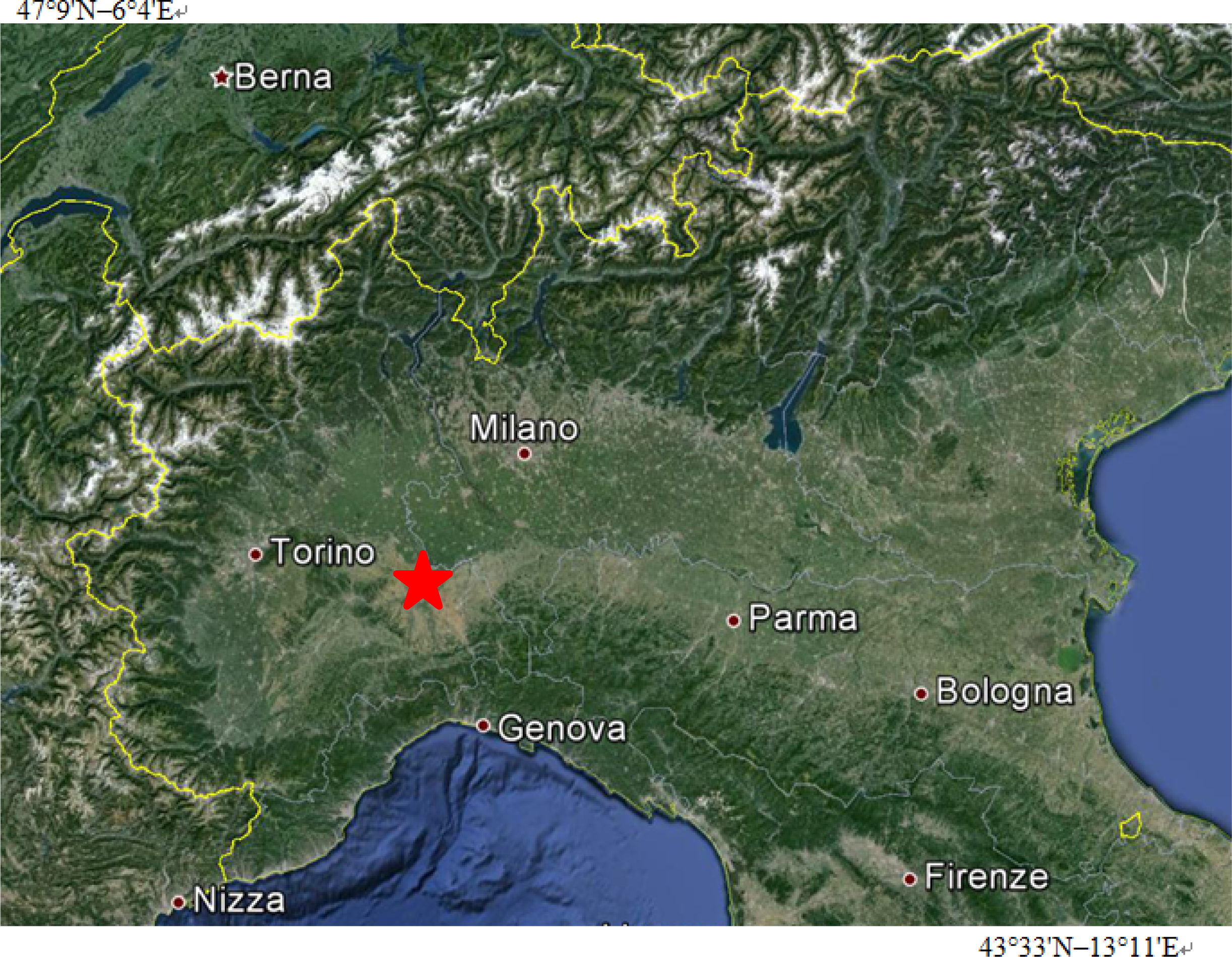
The investigation was carried out on the Scrivia test site, which is located in North-West Italy (central coordinates: 45°N, 8.80°E) (
Figure 1). It is a flat agricultural plain of about 300 km
2, situated close to the confluence of the Scrivia and the Po rivers. The site is characterized by large homogeneous agricultural fields of wheat, corn, sugarbeet, and potatoes [
26]. The weather is generally cloudy and rainy in spring and fall, with average SMC > 0.30–0.35 m
3/m
3, and sunny and dry in summer, with average SMC < 0.15–0.20 m
3/m
3. According to the crop calendar of this area, in fall (October and November) most fields were bare and with SMC > 0.20–0.25 m
3/m
3, whereas in spring (March, April) almost half of the agricultural area was covered by growing wheat. The other half consisted of very rough bare fields, waiting for the seeding of corn. In spring SMC was usually rather high (>0.30 m
3/m
3) due to the frequent rainfall. In May corn was sowed in very smooth fields. These fields were irrigated and therefore their SMC was highly variable. In June–July, the SMC was usually very low (0.10–0.15 m
3/m
3) due to the absence of rainfall, except in the irrigated fields. Wheat was in the ripening phase in June and harvested at the beginning of July.
ENVISAT/ASAR images were mainly collected from 2003 to 2009 in both HH/HV and VV polarizations and at an incidence angle of 23°. In
Table 1 a list of available ENVISAT/ASAR images and their configuration is shown. Simultaneously with satellite acquisitions, ground campaigns were carried out in the sub-area of “Castelnuovo Scrivia”. The ground measurements, mainly collected on 23 “reference” fields, involved all the significant vegetation and soil parameters, such as plant density, leaf and stalk dimensions, the number of leaves per plant, plant water content, SMC, and surface roughness. At least 5–6 samples of SMC (measured with TDR probes, which measure an average SMC of about 10–15 cm, depending on the soil density) and vegetation were collected for each field considered, while surface roughness was measured with a needle profilometer along and across the rows [
26].
3. Retrieval Approach for Estimating SMC from SAR Images
The algorithm used for estimating SMC has already been described in [
26,
27], and it is based on an artificial neural network (ANN) approach. The ANN is a feedforward multilayer perceptron (MLP), with two hidden layers of ten neurons each [
28,
29]. The algorithm was implemented within the framework of an ESA project (4000103855/11/NL/MP/fk) concerning the development of an operative algorithm for the SMC retrieval from Sentinel-1 data.
Studies carried out in the past pointed out that the main constraint for obtaining a good accuracy with ANN approaches is the “robustness” of the training process, which has to be representative of a variety of surface conditions as wide as possible. In order to meet these requirements, the dataset implemented for the ANN training was obtained by combining experimental satellite measurements of backscattering coefficients (σ°) and corresponding ground parameters, derived from the archives available at IFAC and EURAC. Since these datasets were not sufficiently wide for training the ANN and completely setting the neurons and weights, data simulated using electromagnetic forward models have been included in the training set. The backscattering of the bare rough surfaces was obtained using the Advanced Integral Equation Model (AIEM) and Oh model [
30–
32], while the contribution of light vegetation was accounted for by using the “Water Cloud Model” [
33–
35], deriving the information on vegetation water content from the NDVI trough a semi-empirical relationship. Minimum and maximum values of the soil parameters measured during the experimental campaigns (soil moisture and surface roughness) were considered in order to define the range of variability of each soil parameter. The input parameters were the incidence angle (between 20° and 50°), the soil height standard deviation (Hstd, between 1 and 3 cm), the correlation length (Lc, between 4 and 8 cm), the dielectric constant (derived from SMC values between 5% and 45%), and NDVI (between 0.2 and 0.8). Since the relationship between Hstd and Lc is rather complicated and it is difficult to obtain reliable measurements of the Lc parameter, we decided to keep these two quantities independent, associating one random variable with each of these. The consistency between experimental data and model simulations was verified before including the simulated data (more than 10.000 data) in the training set. The ANN training was carried out by considering the simulated backscattering at the various polarizations and the incidence angle as input of the ANN, and the soil parameters as outputs. After training, the ANNs were tested on a different dataset that was obtained by re-iterating the model simulations [
27]. Six ANNs were defined and trained specifically, in order to cover all the possible combinations of input data (
i.e., 1. VV polarization only, without NDVI; 2. HH polarization only, without NDVI; 3. VV polarization and NDVI; 4. HH polarization and NDVI; 5. VV and VH polarizations; 6. HH and HV polarizations). If available, the cross-polarized channel was considered instead of NDVI to account for the effect of dense vegetation cover. The training was carried out by considering the EO data (measured or modeled) as ANN inputs and the SMC as output.
After training, the ANNs were tested on a different dataset, obtained by re-iterating the model simulations. The most favorable results were obtained when co- and cross-polarizations were available, showing a determination coefficient (R
2) equal to 0.80, and RMSE < 0.04 m
3/m
3 [
27]. The ANN algorithm was tested and validated in six main test sites (four in Italy, one in Australia, and one in Spain), where SAR images and simultaneous ground truth data had been collected for several years.
Scrivia,
Matera, and
Spanish sites were agricultural areas, whereas
Cordevole and
Alto Adige were mountainous sites. The
Australian one, which was chosen in order to test the algorithm in meteorological and climatic conditions far from the Italian sites, was characterized by natural pastures and agricultural fields. Detailed descriptions of these areas are given in [
26,
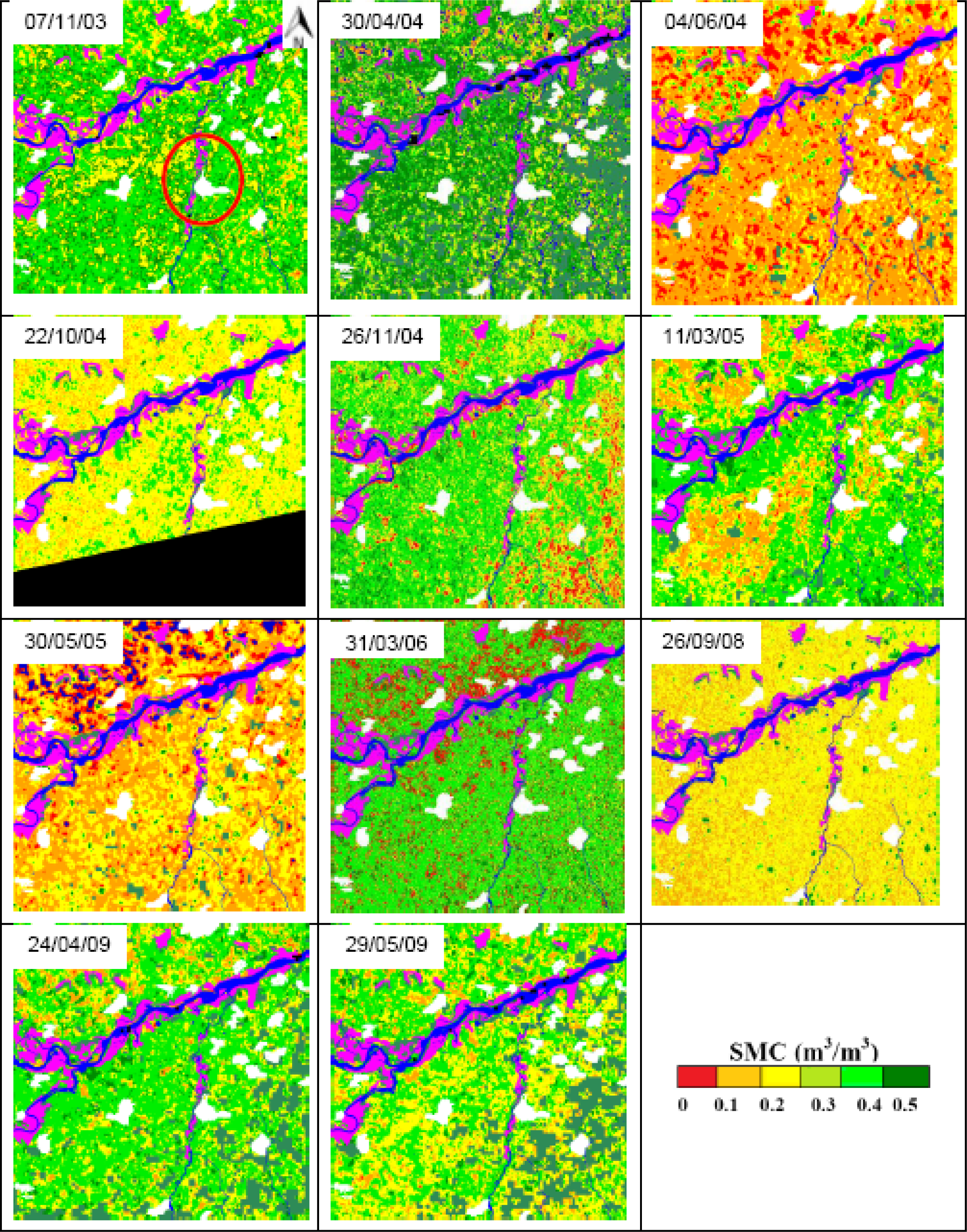
27]. By using the ANN algorithm, a series of SMC maps of the area of Scrivia was generated from the available ENVISAT/ASAR images of
Table 1. The 11 derived maps are shown in
Figure 2. Although SMC data measured on ground are available for only a portion of the image, we can note that the variations of SMC are in agreement with the season, showing a general lower value in summer and a higher value in fall and spring, when rainfall is significant (average monthly rainfall > 100 mm, especially in spring). The areas where SMC the estimate of is not likely,
i.e., urban areas, water bodies, forests, and dense vegetation, were masked with the help of a land use map, combined with a threshold derived from NDVI data. The latter allowed the masking of dense vegetation,
i.e., areas covered by agricultural or natural herbaceous vegetation, dense enough to hamper the SMC retrieval (that of course depended on the growing cycle and changed in time).
In
Table 2, a comparison between SMC values, measured on ground and estimated from SAR data, is shown. The SMC values (both estimated and measured) were averaged over a portion of the image (marked with a red circle) corresponding to the area where ground truth data were collected. The statistical parameters of the regression between these two datasets, although made up by few points, are the following: slope = 0.964, R
2 = 0.91, RMSE = 0.023 m
3/m
3 (p < 0.05). The aim of
Table 2 was to support the SMC maps of
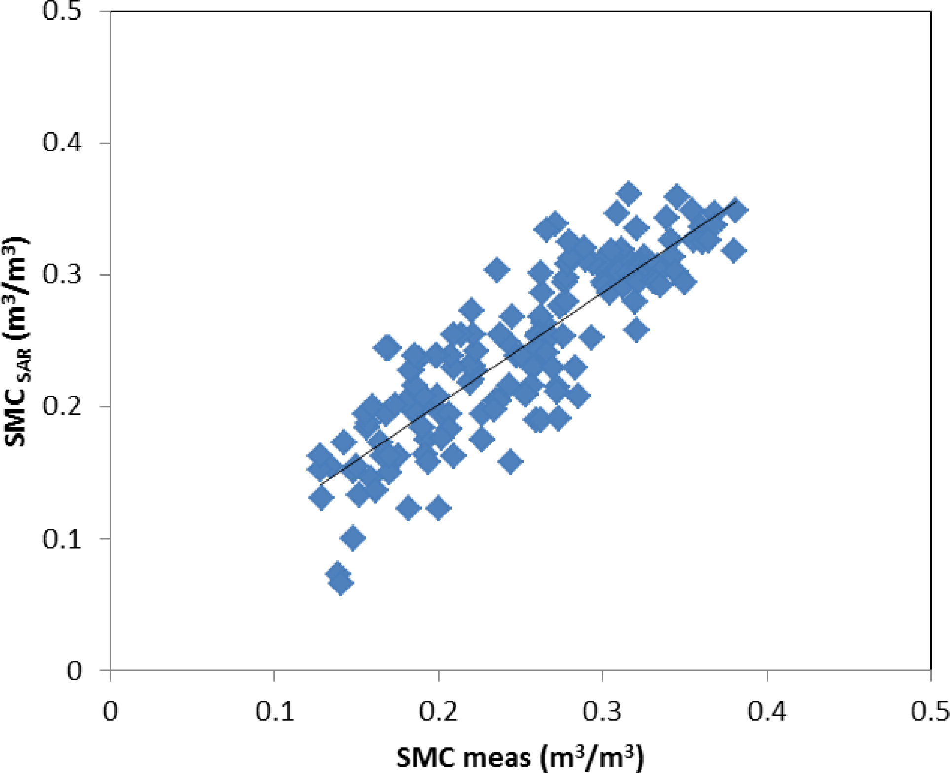
Figure 2, providing an average seasonal trend of SMC. However, looking at a field by field comparison, represented in the diagram of
Figure 3, the following regression line between SMC estimated (SMC
SAR, in m
3/m
3) and SMC measured (SMCmeas, in m
3/m
3) was obtained:
4. Description of the Hydrological Model
In this section, the results of a comparison between SMC SAR estimates and some hydrological model simulations are presented with reference to the test site of Scrivia.
We used the simple daily step model, described in [
36], based on a one-layer soil water balance model, which was found to be able to reasonably reproduce soil moisture variability and has the advantage of describing the top soil layer with simple formulations. The model considers a single, homogeneous, well mixed soil layer for which daily water balance is computed accounting for precipitation, runoff, gravity-driven infiltration and actual evapotranspiration. The model ignores the effect of groundwater, which is usually acceptable for not extremely shallow soils. This simplification should not be applied whenever topsoil moisture is controlled by capillary rise from the water table. In many cases, however, including those considered in the present paper, it may be safely assumed that the water table is sufficiently deep to exclude any significant effect on topsoil moisture. We provide hereafter a short description of the model, extracted from Appendix A in [
36].
The model computes soil volumetric water content variations (1/day) at daily time step as:
In the above expressions, θ
FC = soil volumetric water content at field capacity (−), θ
WP = soil volumetric water content at wilting point (−), PET = potential evapotranspiration (mm/day), L = soil thickness (mm), θ = soil volumetric water content (−), θr = residual soil volumetric water content (−), I
ex = infiltration excess, AET is the actual evapotranspiration, and K(θ) is the saturation-dependent hydraulic conductivity. The model assumes that drainage of the topsoil follows gravity only. Moreover, drainage is not allowed to exceed θ − θ
FC during one time step. Actual evapotranspiration, AET (mm/day), is:
where β is a function that accounts for soil water content during reduced evapotranspiration. In the present formulation, we adopt the SWAT model formulation [
37]:
Saturation-dependent hydraulic conductivity K(θ) is:
which is the well-known Mualem-Van Genuchten model [
38,
39] with tortuosity parameter τ = 0.5, where
Ksat = saturated hydraulic conductivity, mm/day,
n = exponent in Van Genuchten soil water retention curve model.
Infiltration excess is:
where
Sc represents the storage capacity of the soil surface; in the present case, a value of 10 mm was assumed by default; the geometric mean of K
sat and K(Θ) represents an infiltration capacity, which needs to be higher than K(Θ), in order to allow infiltration when soil is in dry conditions. Water in excess of θ
s is computed as:
Runoff (RO) is computed as:
Infiltration (F) is given by:
Day by day, soil water content is updated on the basis of the above calculations. Besides the parameters representing physical characteristics of the soil, which can be in principle determined by experimental measurements, the model requires input of the L parameter (soil thickness).
The minimum set of parameters required as input includes precipitation, mean, minimum and maximum temperature at daily steps and an indication of soil texture. Potential evapotranspiration is estimated using the well-known Hargreaves-Samani formula [
40]. The hydraulic behavior of the top soil layer is described using parameters estimated on the basis of soil texture.
Soils in the test area are predominantly loamy-sands (sand 51%, clay 13%, silt 36%) with a mean bulk density of 1.18 kg/L, according to the soil map of Regione Piemonte (
www.regione.piemonte.it) that was used for this study. Data on precipitation and temperature were obtained from the Agenzia Regionale per la Protezione Ambientale (ARPA) Piemonte station of Castelnuovo Scrivia for the period of interest. Taking precipitation and temperature data from a single station implies ignoring the spatial variability of these parameters, and assuming that the station is representative of the whole area. It is well known that precipitation and temperature vary significantly in space, and such assumption would not be suitable when modeling large catchments, especially with complex topography. For the purposes of our analysis, however, this statement can be considered acceptable, as the spatial extent considered is rather limited, and the local topography is very simple. On the other hand, including data from other, far away measurement stations would introduce extrapolation errors that are not desirable in this context.
Knowing soil properties, hydraulic parameters can be indirectly estimated using pedotransfer rules or expert systems, such as the popular artificial-neural-network-based ROSETTA (
http://cals.arizona.edu/research/rosetta/). After estimating hydraulic properties and the respective standard errors, the ensemble of soil moisture time series, corresponding to all possible combinations of the mean values and values at the extremes of the range for the parameters, may be easily derived. Results of the ensemble of model predictions, measurements, and earth-observation-based estimates will be compared.
5. Comparison of Results and Discussion
For the test site of Scrivia, 11 processed satellite images (see
Table 1) were available, as well as corresponding ground measurements of soil moisture for the same days. The comparison with the hydrological model simulations is not a validation
stricto sensu, but rather a “soft” validation or additional test that served to complement the comparison with ground data. The model provided a continuous simulation of soil moisture that was shown to be in general agreement with the observations. Available SMC measurements could also be used to calibrate the model. Once the model was calibrated for the sites on which data were available, the predicted SMC was compared with the SAR simulated data. The SMC values, both measured and simulated, have been averaged over the area where ground measurements were gathered (see
Figure 2). Since the model referred to the average SMC within the soil layer, while SAR SMC products reflected only shallow soil conditions, a careful examination of the two variables needed to be performed.
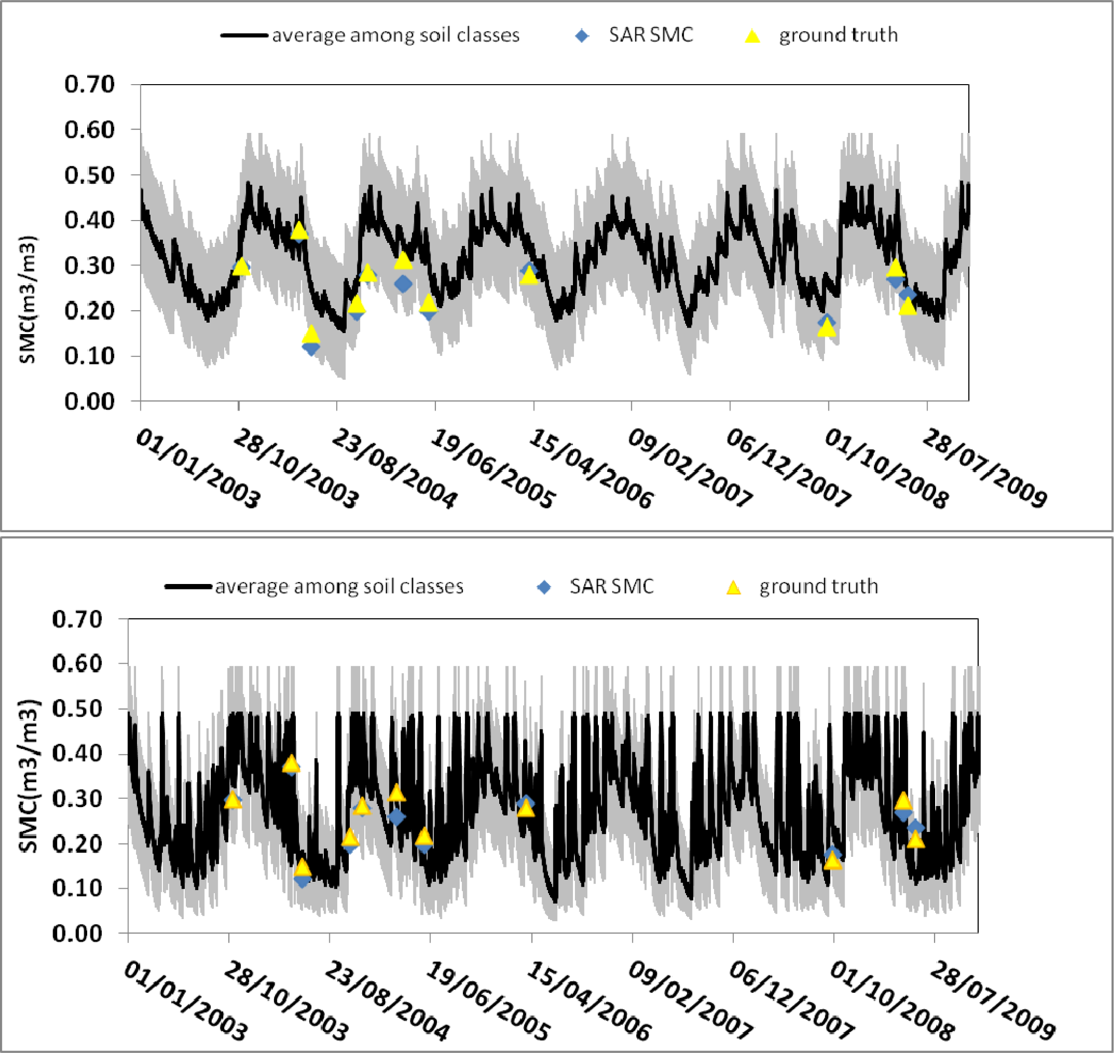
The comparison was carried out by running the hydrological model with parameters for all soil textural classes present in the study area, and by considering the variability of the soil hydraulic parameters estimated by ROSETTA. The latter considered two soil depths: 30 and 5 cm, as depicted in
Figure 4, in which the average and the 95% confidence interval of the resulting simulation ensemble for the two depths were indicated. As clearly appearing from both figures, the 30 cm simulations indicate that SMC values were higher than the satellites estimates, which naturally refer only to the upper layer of soil. In the 5-cm simulations, instead, the agreement between hydrological simulations, satellite estimates and ground measurements may be considered satisfactory.
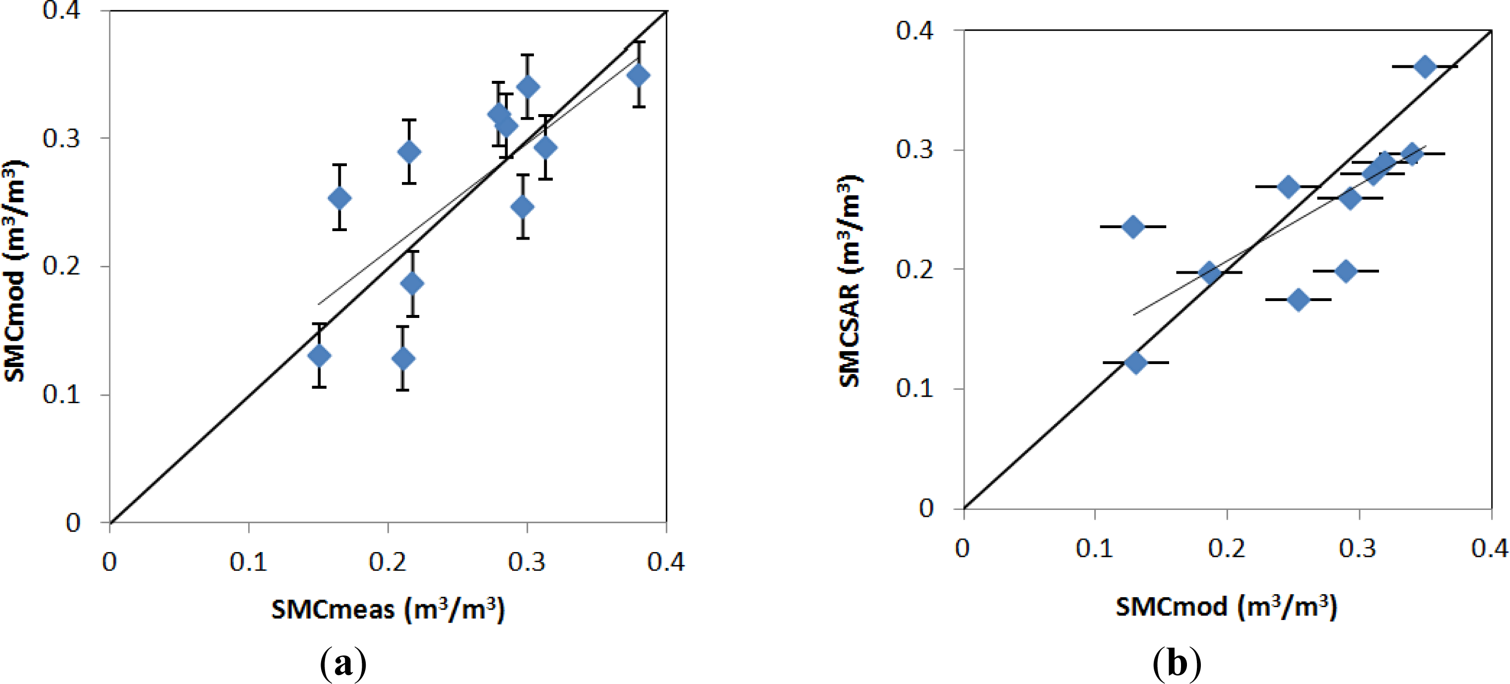
A comparison between the available data was carried out and shown in
Figure 5a, where the SMC estimated with the hydrological model (SMC
mod) was directly compared to SMC measured on ground (SMC
meas). Subsequently, a comparison between SMC
mod and SMC estimated from SAR data (SMC
SAR) was also carried out (
Figure 5b). The obtained regression lines for both diagrams are the following:
Considering the low number of available measurements, these correlations have been found significant, with 95% confidence level (p-value).
In
Table 3, R
2, slope, RMSE, and p of all the correlation carried out between SMC measured on ground, estimated from SAR data and from the model at two depths (5 and 30 cm) are shown. We can note that the best correlation was obtained by directly comparing SMC
SAR and SMC
meas and the worst, at least in terms of RMSE, between SMC
SAR and SMC
mod at 30 cm. It can be observed that the SMC can be better approximated by the hydrological model at 5 cm. The RMSE values range from 0.051 and 0.054 m
3/m
3 for SMC estimated with the hydrological model (at 5 cm depth) and SMC measured on ground and simulated from SAR data, respectively.
Although high spatial resolution products, such as SAR images, usually show a low revisit time, thus hampering their use for simulating soil moisture dynamics, they can be valuable for testing hydrological models and, in particular, hydrological patterns as well as basic assumptions of the model itself. In this view, the test of the soil moisture product with independent hydrological simulations can be considered an interesting result.
6. Conclusions and Future Works
It is well known that microwave remote sensing techniques can provide rather accurate estimates of soil moisture content (SMC). However, the SMC obtained in this way only refers to the first centimeter layer of the soil, thus limiting its assimilation into hydrological models.
In this paper, a comparison between SMC obtained from SAR images, through an inversion algorithm based on an Artificial Neural Network (ANN) approach, and SMC estimated from a hydrological model was performed. The outputs of two models were subsequently compared with field measured SMC. The hydrological model estimated SMC of the two different depths: 30 cm and 5 cm. The first output tended to overestimate the SMC values obtained from SAR images, which, as expected, simulated a shallow SMC. The result of the hydrological model for the first 5 cm depth was instead much more in agreement with satellite data. The RMSE values of these comparisons were 0.052 m3/m3 for the SMC estimated from the hydrological model and 0.023 m3/m3 for the SMC estimated from SAR data.
It is highlighted that products derived from high-temporal frequency satellite images at low spatial resolution have already been used for the assessment of the temporal dynamics of soil moisture. On the other hand, high spatial resolution products, such as those considered in this work, which present lower temporal frequency (and consequently are of limited importance with respect to soil moisture dynamics), may be extremely valuable for testing hydrological patterns and basic assumptions of the models, such as hydrological connectivity and similarity. For these reasons, a deeper investigation on the reliability and compatibility of the soil moisture products derived from SAR images, by using independently derived hydrological simulations, have an important role in hydrological research.
A further comparison between SAR SMC estimates and hydrological model simulations over the Scrivia test site was carried out. The hydrological model reproduced similar values of SMC as compared to the ANN algorithm outputs and ground measurements, provided that the soil layer considered was of the order of only a few centimeters.
The found accuracies of the model simulations, the SAR estimates, and the ground measurements indicate that most of them are within the requested accuracies for satellite products of soil moisture, which, in case of GMES Sentinel-1, is ≤0.05 m3/m3. This result supports the idea that the model simulations may be used as a substitute in case of missing SAR data of dense temporal series or for extending the point-scale measurement of SMC to a more distributed and larger spatial scale.
The comparison conducted in this research can be considered a preliminary exercise, while comparisons with more complex spatially-explicit models should be expanded during future research.

 ,
, 


