Mapping of Ice Motion in Antarctica Using Synthetic-Aperture Radar Data


1
Department of Earth System Science, University of California, Irvine, Irvine, CA 92697, USA
2
Caltech’s Jet Propulsion Laboratory, Pasadena, CA 91109, USA
*
Author to whom correspondence should be addressed.
Remote Sens. 2012, 4(9), 2753-2767; https://doi.org/10.3390/rs4092753
Submission received: 19 July 2012
/
Revised: 30 August 2012
/
Accepted: 4 September 2012
/
Published: 18 September 2012
(This article belongs to the Special Issue Remote Sensing by Synthetic Aperture Radar Technology)
Abstract
:Ice velocity is a fundamental parameter in studying the dynamics of ice sheets. Until recently, no complete mapping of Antarctic ice motion had been available due to calibration uncertainties and lack of basic data. Here, we present a method for calibrating and mosaicking an ensemble of InSAR satellite measurements of ice motion from six sensors: the Japanese ALOS PALSAR, the European Envisat ASAR, ERS-1 and ERS-2, and the Canadian RADARSAT-1 and RADARSAT-2. Ice motion calibration is made difficult by the sparsity of in-situ reference points and the shear size of the study area. A sensor-dependent data stacking scheme is applied to reduce measurement uncertainties. The resulting ice velocity mosaic has errors in magnitude ranging from 1 m/yr in the interior regions to 17 m/yr in coastal sectors and errors in flow direction ranging from less than 0.5° in areas of fast flow to unconstrained direction in sectors of slow motion. It is important to understand how these mosaics are calibrated to understand the inner characteristics of the velocity products as well as to plan future InSAR acquisitions in the Antarctic. As an example, we show that in broad sectors devoid of ice-motion control, it is critical to operate ice motion mapping on a large scale to avoid pitfalls of calibration uncertainties that would make it difficult to obtain quality products and especially construct reliable time series of ice motion needed to detect temporal changes.
1. Introduction
An improved understanding of ice sheet dynamics is essential to the determination of the mass balance of ice sheets and their contributions to sea level [1,2]. Over the past decades, spaceborne Interferometric Synthetic Aperture Radar (InSAR) has revolutionized our ability to detect the surface motion of glaciers and ice sheets (e.g., [3]). This remote sensing technique enables large-scale (100–1,000 km) measurements of ice motion, day and night, independent of cloud cover, at a level of precision comparable or superior to that of kinematic Geographic Positioning System (GPS) (e.g., [4]), at a spatial resolution of a few tens of meters.
InSAR coverage of Antarctica started in 1991 with the launch of the European Earth Remote Sensing Satellite 1 (ERS-1), which provided a wealth of data in the winter of 1995–1996 in tandem with ERS-2. Data coverage was however limited in space by the necessity to be within the mask of a receiving station, in time by the duration of the tandem campaign, and in data volume by the absence of ascending tracks over most of East Antarctica. This made it impractical to obtain high-precision measurements of ice sheet flow over the entire continent. In 1997, RADARSAT-1 imaged regions south of 81°S interferometrically for the first time, including South Pole, after the satellite was rotated to point its radar antenna to the south [5]. The mapping only provided a partial coverage of the South Pole region because InSAR was only used in a demonstration mode at the time, the main mapping activity being to map the radar amplitude of the continent. In 2000, RADARSAT-1 Antarctic Mapping Project (RAMP) acquired data north of 80.1°S repeatedly and interferometrically [6], but the data proved difficult to use in northern West Antarctica, the Antarctic Peninsula and Wilkes Land in East Antarctica, due to high temporal decorrelation of the radar signal. As a result, the RAMP mosaic only provided a partial view of Antarctic ice motion. Overall, the data gathered until 2006 were sufficient to provide a first, comprehensive mapping of glacier velocities near grounding lines [1], but covered less than 30% of the interior regions with quality data.
In the framework of the International Polar Year (IPY) 2007–2009, space agencies in Japan, Canada, Europe and the US formulated a plan to obtain a complete, Pole to Coast, interferometric coverage of the continent. This effort combined the unique imaging capabilities and performance levels of several instruments, including a comprehensive coverage with ALOS PALSAR in 2007–2009 for regions north of 77.5°S, three successive mapping campaigns by ENVISAT ASAR and the first complete coverage of regions around South Pole by RADARSAT-2 in fall 2009.
Here, we present the workflow, i.e., processing, calibration, mosaicking and error estimation, used to generate the first complete ice velocity map of Antarctica based on InSAR data from 6 different platforms. We discuss the method, results, error budget, and impact on the scientific interpretability of the data. We illustrate the practical issues of large scale mosaicking in the context of mapping the flow of ice in the drainage basin of Moscow University Ice Shelf and Totten Glacier in East Antarctica, which is devoid of control points and where detecting temporal changes in ice motion is a special challenge. We conclude on the importance of large-scale mapping processes for glaciological studies.
2. Data
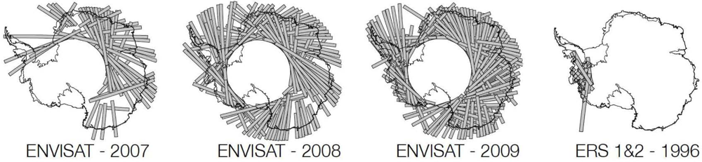
The data contributors to this effort are the European Space Agency (ESA) with Envisat ASAR; the Japan Aerospace Exploration Agency (JAXA) with ALOS PALSAR, and the Canadian Space Agency (CSA) with RADARSAT-2. The ALOS Phased Array-type L-band (λ = 23.6 cm) SAR (PALSAR) was launched in 2006 by JAXA. The data used here were acquired in series of 2 to 3 consecutive passes over 4 time periods: from May to September 2006, from November 2006 to January 2007, from September 2007 to January 2008 and from September 2008 to January 2009. The data were obtained as raw individual frames from JAXA via the Alaska Satellite Facility (ASF). Despite the 46-day repeat cycle of the mission, the long radar wavelength of PALSAR yields high temporal coherence even along wet sectors. This dataset is the largest in terms of data volume (see Table 1) and provides SAR coverage north of 77.5°S (Figure 1).
The Advanced Synthetic Aperture Radar (ASAR) launched in 2002 by ESA operates on a 35-day repeat, operated at C-band (λ = 5.5 cm) onboard ENVISAT. It covers Antarctica up to 79°S. Two consecutive passes per year for each track were made over Antarctica each year between 2007 and 2010 included. We use data from 3 campaigns spanning May–August 2007, May–August 2008 and May–August 2009. The data were distributed to us by ESA. A special effort was made by ESA, for the first time, to acquire and distribute coast-to-coast tracks.
The RADARSAT-2 SAR has a 24 day repeat cycle, operates at C-band (λ = 5.5 cm) and is the only sensor with a left looking capability capable of imaging South Pole. RADARSAT-2 was launched by CSA in December 2007 and CSA focused the RADARSAT-2 data collection effort on areas south of 77.5°S. A second campaign was executed in 2011 to fill in remaining gaps that could not be imaged in the first campaign. This provided the first complete InSAR coverage of this sector.
The 46-day repeat L-band PALSAR data displays higher correlation than the 24- or 35-day repeat C-band data. On the other hand, PALSAR data are affected by ionospheric noise, especially near the magnetic South Pole in East Antarctica. PALSAR is most useful to map coastal sectors of high flow speed and high surface weathering, whereas C-band data is more appropriate for slow moving sectors with low surface weathering. Despite the comprehensive coverage of the continent with the 3 aforementioned satellites, some gaps remained due to lack of data or poor coherence. A portion of these gaps were filled using RADARSAT-1 (CSA) and ERS-1/2 data (ESA), however this process could only be applied in areas with very low probability of velocity change (Figure 1).
The SAR data from 5 sensors, except RADARSAT-2, are delivered in raw (signal and telemetry) format, frame by frame (about 100 km-long segments). The data are processed into single look complex (SLC) data using the Gamma Remote Sensing processor ( http://www.gamma-rs.ch). Further data analysis is pursued using our own processing methodology described next.
3. Methods
3.1. Speckle Tracking
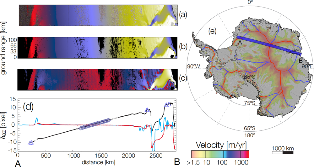
We apply a speckle tracking technique [7] on SAR image pairs to derive slant range and azimuth vector displacements (δrg and δaz, respectively) with a sub-pixel quantization noise of 1/128 th of a pixel; in practice, we achieve a noise level of 1/100 th of a pixel (Figure 2(a)). The cross-correlation program is a modified version of
ampcor from the JPL/Caltech repeat orbit interferometry package (
ROI_PAC) [8]. Speckle tracking is performed on sub-images 600 m (range) × 1,000 m (azimuth) in size, on a regular grid with a grid spacing of 150 m × 300 m, and a search domain, which is size dependent on flow speed, i.e., a larger search window is used for larger offsets. The offsets are median filtered to remove poor matches. To do so, we eliminate pixels for which the pixel offsets deviate more than 3 units from offsets filtered by a 9 pixel × 9 pixel median filter (see Figure 2(a,b)).
3.2. Calibration
The components of surface ice displacement (δx, δy, δz) in a local Cartesian coordinate system are estimated from the slant range and azimuth displacements, δrg and δaz respectively, as:
where σirg and σ iaz are the ionospheric noise contributions; σBrg and σ Baz are the residual errors in interferometric baseline in range and azimuth; θ is the incidence angle with respect to the local vertical direction; and ∊rg and ∊az are residual noise contributions in range and azimuth.
Ionospheric disturbances cause phase gradient resulting in azimuth shifts, called “azimuth streaks” [10]. Large scale variations of the total electron content of the ionosphere also yield slight range shifts between the SAR images [11]. We tested several methods of ionospheric noise estimation and removal but did not converge on a viable technique that could be employed over the entire dataset. Ionosphere perturbations are proportional to the radar wavelength squared, hence are 16 times stronger at L-band than C-band. Instead of removing ionospheric errors from the L-band data, we combined L- and C-band results in a manner that reduces their noise, as described below.
Assuming surface-parallel ice flow, the vertical surface displacement δz is related to the horizontal displacements by:
where αaz and αrg are the surface slopes in the azimuth and range directions, respectively.
The residual baselines (σBrg, σBaz) are modeled as two-dimensioned quadratic polynomial functions as:
where krgi,j and kazi,j are the polynomial coefficients, rg and az are respectively the slant range and azimuth position in the offset map, and i and j are the polynomial exponents for slant range and azimuth, respectively.
At present, satellite orbits are not known sufficiently well to know the baseline perfectly. Residual errors must be estimated and removed. The traditional method is to select points of known velocity along the track to best fit a quadratic baseline in the least-square sense. In the absence of a large quantity of in situ measurements of ice motion, we rely on areas of zero motion. These areas include ice islands, emergent mountains, exposed rock outcrops, domes, and ice divides with near-zero (<0.1°) surface slope. In addition, we employ balance velocity [12] for regions where speed is less than 10 m/yr (Figure 2(e)). Baseline calibration is easy in the Antarctic Peninsula, where coast-to-coast acquisitions are routinely available and many zones of emergent rock are available. It is also not difficult in West Antarctica. It is however challenging in East Antarctica, when areas of zero motion are sparse, separated by long distances and not known a priori. Balance velocity is used in East Antarctica to help circumvent the lack of zero-motion control points.
We use coast-to-coast ASAR tracks (Figure 3(e)) to create a set of reference tracks in the ice sheet interior. These tracks maintain high signal coherence across the entire continent, have low ionospheric noise and intercept areas of zero motion along the coasts as well as in the interior (ice divides). For each track individually, calibration is achieved by least square adjustment of the quadratic baseline as defined in Equation (3), separately for the range and azimuth components, using a large number of zero-motion control points. Selecting a large number of points helps minimize the error. Up to 5 iterations are necessary for the solution to converge to a suitable set of reference tracks (Figure 3(a)). This iteration process is stopped when the ice speed on areas of zero motion and the differences between overlapping tracks are typically of the same order of magnitude as the noise level (±4 m/yr for ENVISAT tracks [13]).
Using Equations (1) and (2), the results are subsequently translated into ground-range and azimuth displacements and converted into a three-dimensional ice displacement vector (δx, δy and δz). This process employs a digital elevation model of Antarctica, here from [9]. Geocoded tracks are assembled in a reference mosaic at 300 m spacing in Polar Stereographic projection with true scale at 71°S and a central meridian at zero degree longitude. Assuming a constant displacement between acquisitions, the ice velocity v in meters per year is calculated as vx,y,z = 365.25 δx,y,z/T, where T is the time interval in days between image acquisitions.
In a second step, the geo-coded calibrated reference mosaic is transformed backward from map projection to radar coordinates for each crossing track. Then, the reference velocity and additional control points are fitted using Equation (3) and geo-referenced as described above. In this manner, using both control points of zero motion and reference points provided by the reference mosaic, we progressively add new radar tracks to the mosaic. The entire calibration process is done in the slant range, azimuth planes of the radar data. We use up to 5 iterations of these steps until the process converges toward a stable solution for the interferometric baselines. The quality of convergence of the solution is illustrated by the excellent consistency between adjacent tracks, across different sensors, and at track crossings in the vast interior of East Antarctica (Figure 3(c)). The fact that a stable solution exists for the interferometric baselines is a strong indicator that the calibration and mosaicking processes are performed correctly.
3.3. Combining Speckle Tracking and Interferometric Phase
We routinely form an interferogram for every pair of acquisition. The range offsets from speckle tracking and the phase from the interferogram are measuring the same displacement in range. The interferometric phase is one order of magnitude more accurate than the range offset but phase unwrapping is not always possible in areas of rapid flow. Wherever it is possible to unwrap the phase, we replace the range offset δrg with the interferometric phase to improve the quality of the results. From the phase and the azimuth offset, the 3-D ice velocity vx,y,z is then computed as described previously.
3.4. Gap Filling with Historic Data
While the IPY data acquisitions provide a complete data coverage of Antarctica, residual gaps exist due to low signal correlation in areas of high surface weathering, such as the Hollick–Kenyon Plateau between Thwaites, Smith and Pine Island Glaciers, the divide of Bakutis Coast, Bryan Coast, the Antarctic Peninsula divide and the Law Dome sector (Figure 3(a–c)).
To fill these gaps, we used data from ERS-1 and ERS-2 in 1996 and RADARSAT-1 in 1997 and 2000. For ERS-1 and ERS-2, the interferometric phase is always used instead of the offsets, because the ERS repeat cycle (1 day) is too short to estimate accurate ice-motion from speckle tracking. Assuming that the velocity vector is parallel to the ice surface, the 3-D ice velocity is derived from interferometric observations collecting in two independent directions (ascending and descending orbits) [15] and the surface slope [9]. Using the combination of ascending/descending passes, we estimate ice-motion over the Rutford ice stream or Carlson Inlet (Figure 1). Each interferogram is calibrated using the speckle tracking mosaic from ASAR, PALSAR and RADARSAT-2 datasets as described previously. RADARSAT-1 is used to complete the coverage of Ronne–Filchner and Riiser-Larsen ice shelves.
4. Results
4.1. Error Analysis
The resulting mosaic uses 1,400 tracks representing more than 3,000 orbits or 30 TByte of raw data. The individual SAR missions differ in their respective technical details (see Table 1), however each sensor contributes uniquely to the complete coverage (Figure 1). To increase the quality of the final map, we implement a sensor-dependent data stacking scheme and attribute a weight to each sensor depending on the ionospheric perturbation, the decorrelation, the accuracy and the acquisition period (see Supplement Online Material in [13]).
Temporal decorrelation is the largest source of noise in repeat pass InSAR. Other noise sources include baseline decorrelation, thermal decorrelation and processing factors [16]. The loss of temporal coherence is influenced by the repeat cycle of the radar and the radar frequency. At a given frequency, coherence decreases when the repeat cycle increases, hence RADARSAT-1 and RADARSAT-2 24-day repeat data yield better coherence levels than ASAR 35-day repeat data. On the other hand, a longer repeat cycle increases the measurement accuracy because it detects a larger displacement with the same absolute precision.
The L-band data are less affected by changes in ice sheet surface properties than C-band data because they penetrate deeper into the surface and temporal coherence is systematically higher [17]. Exceptions includes radar-dark areas, i.e., areas of high snowfall, and areas affected by strong ionospheric perturbations. In some areas, the ionospheric noise exceeds the actual signal (Figure 3(b)). On average, PALSAR ionospheric errors are ±17 m/yr near magnetic pole where precipitation of energetic solar particles is intense, and ±8 m/yr in West Antarctica Ice Sheet (WAIS) (see Supplement Online Material in [13]). At C-band, ionospheric errors contribute maximum velocity errors of ±6 m/yr for RADARSAT and ±4 m/yr for ENVISAT.
In East Antarctica where ionosphere perturbations are significant, we therefore increase the weight of C-band data versus L-band. In West Antarctica, we do the opposite. Historic data, ERS-1&2 and RADARSAT-1 are given a low weight so they only contribute where no other sensor provides data.
We mosaic the different data by averaging them with a sensor specific weight wi as defined:
where v = (vx, vy) is the mean velocity (each component is calculated separately), vi and wi are respectively the velocity and weight of each individual track, σv is the error associated with v, and σi is the error attributed to each track as discussed above.
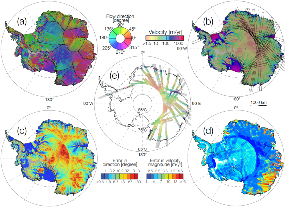
In few areas where the number of stacked data is high, the resulting error σv converges to zero, which is unrealistic and underestimates the actual error. For instance, the standard deviation of the ice speed measured in a sector of zero motion and large number (>20) of stacked tracks is 0.989 m/yr. We therefore force the error σv to always exceed 1 m/y. The error mosaic map is displayed in Figure 3(f). The largest errors are found along the coast of East Antarctica, which is only covered with PALSAR and where ionospheric noise is high. The lowest errors are found in the interior of East Antarctica (up to 79°S) where ASAR tracks overlap up to 36 times.
As a result of the sensor-dependent mosaicking, we obtain a reference, comprehensive, high-resolution, digital mosaic of ice motion (vx,vy,vz) in Antarctica assembled from multiple satellite interferometric synthetic-aperture radar (Figure 3(e)). The map reveals widespread, enhanced flow with tributary ice streams reaching hundreds to thousands of kilometers inland [13].
We also calculate the flow direction θ (Figure 3(a)) and the associated error σθ (Figure 3(c)) as:
where θ is the direction of the flow in radians (with respect to the x-axis), vx and vy are, respectively, the velocity magnitude along x and y axis in a local Cartesian system, and σθ (in radians), σvx and σ vy are the errors associated with θ, vx and vy, respectively. If we define the velocity magnitude v as
and, if we assume that the associated error σv is approximated by
, the previous equation is rewritten as:
Flow direction precision is excellent near the coast where errors are below 1° (Figure 3(c)). The error increases as the velocity magnitude decreases and the flow direction is essentially unconstrained when errors in magnitude are comparable to the velocity magnitude near major ice divides.
To perform the translation of offset measurements to three dimensional ice displacement vectors, we use a digital elevation model (DEM) from [9]. Absolute errors in the DEM used for processing introduce only small errors in velocity, but slope errors can produce errors of up to 3% of the observed speed [18]. The DEM errors are discussed in [19]. Errors in the DEM are negligible over the ice shelves and for the majority of the grounded ice sheet (1 m and 2–6 m, respectively). Along the Peninsula and mountain ranges the estimated DEM error is several tens of meters and could therefore affect the ice velocity.
4.2. Validation
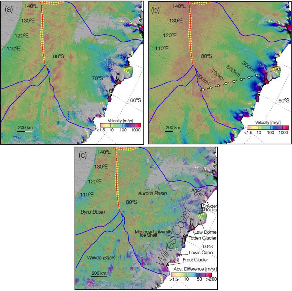
Figure 3(b) illustrates a fortiori the difficulty of calibrating ice velocity at the regional scale, especially in East Antarctica where few natural targets of zero motion are available or known. The large drainage basins particularly challenging to process include Byrd, Cook, Recovery, Slessor, or Aurora shown in Figure 4. For example, the coastline of the Aurora basin consists mainly of ice cliffs interrupted by large discharge glaciers such as Moscow University Ice Shelf, Totten and Frost Glaciers contrasting with regular outlet glaciers because of the absence of rock exposures. On the 1,300 km of coast in this sector, only three non-moving targets are well known: Lewis Cape, Law Dome, Snyder Rocks; the others correspond to stagnant areas that had never been discussed in the literature (see Figure 4(a)). They include an ice rise at the end of the Totten Glacier Tongue and an unnamed island that buttresses Moscow University Ice Shelf for several hundred kilometers. These new features were subsequently used to improve calibration in new iterations. The interior of this sector has no rock outcrops or nunataks and control points of zero surface slope are thousands of kilometers away. Thus, the geographical characteristics of Aurora basin requires long tracks and the calibration of the entire basin to obtain enough control points to constrain ice velocity. The final result is shown in Figure 4(b).
To illustrate the improvements in velocity precision of our calibration approach, we compare our result in the sector of Aurora basin (Figure 4(b)) with the large scale mapping RAMP (Figure 4(a)) [6]. During RAMP, three full cycles covering the area north of 80°S were acquired to generate an ice velocity product. The difference between the two datasets is shown in Figure 4(c). RAMP velocities roughly agree with our study in the interior regions, but differences >40 m/yr are found in the Byrd, Aurora or Wilkes basins, and up to 100 m/yr along the divide between Wilkes and Aurora basins. Closer to the coast, differences >60 m/yr are common. For instance, the velocity difference is 90 m/yr between RAMP and IPY on Frost Glacier, 60–70 m/yr upstream the Totten grounding line and ranges from −100 to 90 m/yr along Knox Coast. These irregularities in speed are even visible in the RAMP velocities (Figure 4(a)). Due to limited data coverage (single sensor, single frequency, single year) and lack of correlation along the coast, the calibration of RAMP velocity is not reliable in this sector.
5. Discussion
Our mosaic is the largest and most complete map of ice motion ever assembled in Antarctica and represents a vast improvement over previous efforts to map ice velocity in Antarctica. This result would not have been possible without the large amount data available for IPY and a specific calibration approach. Our methodology relies on the availability of coast-to-coast tracks, quadratic baseline estimation, and the implementation of a sensor-dependent data stacking scheme to minimize errors. Topographic divides, stagnant coastal features and calculated balance velocity near ice divides (<10 m/yr) serve as control points for calibration. Data calibration would be difficult—if not impossible—to achieve in the absence of coast-to-coast tracks, which were first acquired by ASAR in 2007. The data calibration approach is sensor independent, so that our results effectively achieve multi-sensor synergy to construct the ice motion product.
To illustrate the need for long tracks of data acquisition and for calibrating entire drainage basins in order to obtain reliable products, we analyzed the influence of track length on the calibration of ice motion of Totten Glacier, in East Antarctica and how the results affect the estimation of its ice flux at the grounding line. When short tracks are used, without knowledge of natural targets of zero motion, the default calibration is to set the farthest point from the coast at zero velocity. This was done along an ALOS PALSAR track between Law Dome (stagnant) and the end point of the track, by varying the track length (Figure 4(b)). The results are shown in Table 2 as the average error in grounding line speed in percent and the corresponding error in ice flux. A reference ice flux of 73.6 Gt is used from [1]. The results show that tracks longer than 600 km are needed to obtain a flux error below 1%. Flux errors increase rapidly with shorter tracks, reaching almost 10% for a 300 km long track. Hence, high-precision data calibration in this region is not possible unless long tracks of InSAR data are acquired. This is especially important in the context of change detection, for instance to detect the speed-up of Totten Glacier over time. If short tracks of InSAR data are employed, it is essentially not practical to detect velocity changes in that basin.
In the future, the IPY map may serve as reference for data calibration, unless major temporal changes in speed are taking place; this greatly facilitates data calibration. The current mosaic could be further improved by adding new data, e.g., ALOS PALSAR from fall 2009 and 2010 and ENVISAT ASAR data from fall 2010. In parts of Antarctica where signal coherence is low, data acquired on a shorter repeat cycle are however required. This is the case of Law Dome in East Antarctica, West Ice Shelf in East Antarctica, the interior of Bakutis Coast in West Antarctica, the upper part of the Pine Island and Thwaites basins, and the western flank of the Antarctic Peninsula. The Western Peninsula and Bakutis coast could be mapped using ERS-1/2 1996 tandem data, but in the other sectors, no data is currently available to fill in the gaps.
In 2013, JAXA will launch ALOS-2 PALSAR-2 on a 14-day repeat cycle, which will be very useful for ice sheet motion mapping. The Radarsat Constellation Mission (RCM) will offer repeat cycles shorter than 24 days in a few years as well. ESA will launch SENTINEL-1 in 2013–2014, on a 12-day repeat cycle to be followed by a second satellite a few years later, hence providing a 6-day repeat cycle which should be of great significance for ice sheet research. Finally, TerraSAR-X is currently providing shorter repeat cycle data, but only over small areas. These satellite missions offer significant opportunities to improve the precision of ice motion mapping in Antarctica in years to come.
6. Conclusions
This paper presents a method for calibrating and mosaicking ice surface motion over the entire continent of Antarctica using 6 different SAR sensors in the framework of the International Polar Year 2007–2009: the Japanese ALOS PALSAR, the European Envisat ASAR, ERS-1 and ERS-2, and the Canadian RADARSAT-1 and RADARSAT-2. The resulting mosaic uses 1,400 tracks representing more than 3,000 orbits. Our methodology relies on the availability of coast-to-coast tracks, quadratic baseline estimation, and the implementation of a sensor-dependent data stacking scheme to minimize errors. We have demonstrated how this could be applied to a large-scale mapping problem and documented the achieved precision of the products, which is an information of great interest to modelers and glaciologists who will use the data for their research work. The resulting ice velocity mosaic has errors in magnitude ranging from 1 m/yr in the interior regions to 17 m/yr in coastal sectors and errors in flow direction ranging from less than 0.5° in areas of fast flow to unconstrained direction in sectors of slow motion. The fact that six sensors were needed for this task illustrates the complexity of ice motion mapping in the continent, and suggest that it is inherently difficult to map the entire continent using data from a single SAR mission. Our calibration strategy highlights major constraints on data acquisition that need to be taken into account for future mission surveys. For instance, coast-to-coast tracks are critical for calibration, especially in East Antarctica. Similarly, shorter repeat cycle are needed to fill in residual gaps where prior data with long repeat cycles fail to provide high signal coherence. We also note that a significant amount of overlap is needed between adjacent tracks from the same or different missions in order to enable the large-scale mosaicking of the data. Our velocity map is a new Earth Science Data Record (ESDR) which is available publicly via institutional links at the National Snow and Ice Data Center [21].
Acknowledgments
This work was performed at the University of California Irvine and at Caltech’s Jet Propulsion Laboratory under a contract with the National Aeronautics and Space Administration’s MEaSUREs and Cryospheric Science Programs. Data acquisitions are courtesy of the IPY Space Task Group. We thank the two anonymous reviewers and the editor for their constructive comments on this manuscript.
References
- Rignot, E.; Bamber, J.L.; van den Broeke, M.R.; Davis, C.; Li, Y.; van de Berg, W.J.; van Meijgaard, E. Recent Antarctic ice mass loss from radar interferometry and regional climate modelling. Nat. Geosci 2008, 1, 106–110. [Google Scholar]
- Rignot, E.; Velicogna, I.; van den Broeke, M.R.; Monaghan, A.; Lenaerts, J. Acceleration of the contribution of the Greenland and Antarctic ice sheets to sea level rise. Geophys. Res. Lett, 2011. [Google Scholar] [CrossRef]
- Joughin, I.; Smith, B.E.; Abdalati, W. Glaciological advances made with interferometric synthetic aperture radar. J. Glaciol 2011, 56, 1026–1042. [Google Scholar]
- Rignot, E. Radar interferometry detection of hinge-line migration on Rutford Ice Stream and Carlson Inlet, Antarctica. Ann. Glaciol 1998, 27, 25–32. [Google Scholar]
- Jezek, K.C. Glaciological properties of the Antarctic ice sheet from RADARSAT-1 synthetic aperture radar imagery. Ann. Glaciol 1999, 29, 286–290. [Google Scholar]
- Jezek, K.C.; Farness, K.; Carande, R.; Wu, X.; Labelle-Hamer, N. RADARSAT 1 synthetic aperture radar observations of Antarctica: Modified Antarctic mapping mission, 2000. Radio Sci, 2003. [Google Scholar] [CrossRef]
- Michel, R.; Rignot, E. Flow of Glaciar Moreno, Argentina, from repeat-pass Shuttle Imaging Radar images: Comparison of the phase correlation method with radar interferometry. J. Glaciol 1999, 45, 93–100. [Google Scholar]
- Rosen, P.A.; Henley, S.; Peltzer, G.; Simons, M. Update repeat orbit interferometry package released. EOS Trans. AGU 2004, 85, 47. [Google Scholar]
- Bamber, J.L.; Gomez-Dans, J.L.; Griggs, J.A. A new 1 km digital elevation model of the Antarctic derived from combined satellite radar and laser data—Part 1: Data and methods. Cryosphere 2009, 3, 101–111. [Google Scholar]
- Gray, A.L.; Mattar, K.E.; Sofko, G. Influence of ionospheric electron density fluctuations on satellite radar interferometry. Geophys. Res. Lett, 2000. [Google Scholar] [CrossRef]
- Meyer, F.; Bamler, R.; Jakowski, N.; Fritz, T. The potential of low-frequency SAR systems for mapping ionospheric TEC distributions. IEEE Geosci. Remote Sens. Lett 2006, 3, 560–564. [Google Scholar]
- Bamber, J.L.; Vaughan, D.G.; Joughin, I. Widespread complex flow in the interior of the antarctic ice sheet. Science 2000, 287, 1248–1250. [Google Scholar]
- Rignot, E.; Mouginot, J.; Scheuchl, B. Ice flow of the Antarctic ice sheet. Science 2011, 333, 1427–1430. [Google Scholar]
- Haran, T.; Bohlander, J.; Scambos, T.; Painter, T.; Fahnestock, M. MODIS Mosaic of Antarctica (MOA) Image Map; National Snow and Ice Data Center Digital Media: Boulder, CO, USA, 2006. [Google Scholar]
- Joughin, I.R.; Kwok, R.; Fahnestock, M.A. Interferometric estimation of three-dimensional ice-flow using ascending and descending passes. IEEE Trans. Geosci. Remote Sens 1998, 36, 25–37. [Google Scholar]
- Hoen, W.E.; Zebker, H. Penetration depths inferred from interferometric volume decorrelation observed over the Greenland Ice Sheet. IEEE Trans. Geosci. Remote Sens 2000, 38, 2571–2583. [Google Scholar]
- Rignot, E.; Echelmeyer, K.; Krabill, W. Penetration depth of interferometric synthetic-aperture radar signals in snow and ice. Geophys. Res. Lett 2001, 28, 3501–3504. [Google Scholar]
- Joughin, I. Ice-sheet velocity mapping: A combined interferometric and speckle-tracking approach. Ann. Glaciol 2002, 34, 195–201. [Google Scholar]
- Griggs, J.A.; Bamber, J.L. A new 1 km digital elevation model of Antarctica derived from combined radar and laser data—Part 2: Validation and error estimates. Cryosphere 2009, 3, 113–123. [Google Scholar]
- Rignot, E.; Mouginot, J.; Scheuchl, B. Antarctic grounding line mapping from differential satellite radar interferometry. Geophys. Res. Lett, 2011. [Google Scholar] [CrossRef]
- Rignot, E.; Mouginot, J.; Scheuchl, B. MEaSUREs InSAR-Based Antarctica Velocity Map; NASA EOSDIS DAAC at NSIDC: Boulder, CO, USA, 2011. [Google Scholar]
Figure 1.
Maps of Antarctica with the footprint of processed tracks for each year employed in this study. More tracks are available, especially for RADARSAT-1, ERS-1/-2 and ALOS PALSAR. Maps are displayed in south polar stereographic projection.
Figure 1.
Maps of Antarctica with the footprint of processed tracks for each year employed in this study. More tracks are available, especially for RADARSAT-1, ERS-1/-2 and ALOS PALSAR. Maps are displayed in south polar stereographic projection.


Figure 2.
From top to bottom, (a) azimuth initial offsets (δaz); (b) offsets after median filtering; (c) offsets after calibration; (d) initial (black line) and calibrated (red line) azimuth offsets versus azimuth; triangles denote zero-motion control points; diamonds indicate where balance velocity (blue line) is used as a reference; 1 azimuth pixel = 4.0 m; (e) Map of Antarctic balance velocity for speed < 10 m/yr [9] with topographic divides (red lines for slope < 0.1°, blue otherwise). The footprint of track A-B is in blue.

Figure 3.
(a) Flow direction for the IPY map, black lines represent major topographic divides; (b) Antarctic ice speed; (c) error in flow direction; (d) error in velocity magnitude or speed; (e) set of ENVISAT reference tracks used for calibration, track outlines also shown in (b). Color coding in (b) and (c) is on a logarithmic scale. Maps (a–c) are overlaid on a MODIS mosaic of Antarctica (MOA) [14]. Maps are displayed in south polar stereographic projection.

Figure 4.
Ice velocity of the Wilkes Land sector using polar stereographic projection and overlaid on MOA, from (a) RAMP in year 2000 [6]; (b) IPY [13]; (c) difference between RAMP and IPY. Control points of zero motion are in dashed yellow. Topographic divides are in blue and red as described in Figure 2. The solid black line in (a–c) is the InSAR grounding line [20]. The dashed black line in (b) indicates the position of the velocity line used in Table 2; white markers correspond to control point locations (Table 2).

Table 1.
Characteristics of the SAR instruments used in this study. Left-looking capability provides the opportunity to cover areas south of 80°S. Details about the acquisition modes can be found on the agency websites. Repeat Cycle corresponds to the period between two consecutive acquisitions. The incidence angle is the angle defined by the incident radar beam and the vertical (normal) to the intercepting surface. Spacing are given for single look complex images.
| Platform | Look Dir. | Mode | Repeat Cycle [day] | Incidence Angle [degree] | Spacing Rg×Az [m] | Swath [km] | Frequency [GHz] | # of tracks | Raw data volume [Tbyte] | Season Year |
|---|---|---|---|---|---|---|---|---|---|---|
| ERS-1 & -2 | Right | IS2 | 1 | 23 | 13×4 | 100 | 5.3 | 60 | 0.5 | Spring 1996 |
| RADARSAT-1 | Left | S2–S7 | 24 | 28–47 1 | 12×5–17×6 1 | 100 | 5.3 | 72 | 0.5 | Fall 1997 |
| Right | various | 24 | 18–38 1 | 7×5–12×5 1 | 50–100 1 | 5.3 | 84 | 0.5 | Fall 2000 | |
| ENVISAT | Right | IS2 | 35 | 23 | 13×5 | 100 | 5.331 | 115/130/210 2 | 1/1/2 2 | Summer 2007/2008/2009 |
| RADARSAT-2 | Left | S5-EH4 | 24 | 41–57 1 | 12×5–12×5 1 | 100 | 5.405 | 135/14 2 | 4/1 2 | Spring 2009/2011 |
| ALOS/PALSAR | Right | FBS | 46 | 39 | 7×4 | 70 | 1.27 | 64/204/296 2 | 2/6/9 2 | Fall 2006/2007/2008 |
1Multiple values correspond to different acquisition modes. See the column “Mode”;
2Multiple values correspond to different years. See the column “Season/Year”.
Table 2.
Influence of the track length on the velocity calibration for Totten Glacier. The second column indicates the reference velocity at the end of the track (the white markers in Figure 4(b)). Totten flux taken as 73.6 Gt from [1].
| Track Length [km] | Velocity [m/yr] | Speed Error Flux at the GL [%] | Error [Gt/yr] |
|---|---|---|---|
| 1,000 | 1.8 | >0.1 | >0.1 |
| 900 | 6.4 | 0.3 | 0.2 |
| 800 | 4.3 | 0.2 | 0.2 |
| 700 | 4.3 | 0.3 | 0.2 |
| 600 | 7.1 | 0.5 | 0.4 |
| 500 | 22.4 | 1.8 | 1.4 |
| 400 | 43.9 | 4.5 | 3.3 |
| 300 | 65.8 | 9.0 | 6.7 |
Share and Cite
MDPI and ACS Style
Mouginot, J.; Scheuchl, B.; Rignot, E. Mapping of Ice Motion in Antarctica Using Synthetic-Aperture Radar Data. Remote Sens. 2012, 4, 2753-2767. https://doi.org/10.3390/rs4092753
AMA Style
Mouginot J, Scheuchl B, Rignot E. Mapping of Ice Motion in Antarctica Using Synthetic-Aperture Radar Data. Remote Sensing. 2012; 4(9):2753-2767. https://doi.org/10.3390/rs4092753
Chicago/Turabian StyleMouginot, Jeremie, Bernd Scheuchl, and Eric Rignot. 2012. "Mapping of Ice Motion in Antarctica Using Synthetic-Aperture Radar Data" Remote Sensing 4, no. 9: 2753-2767. https://doi.org/10.3390/rs4092753