Monitoring Biennial Bearing Effect on Coffee Yield Using MODIS Remote Sensing Imagery
by
Tiago Bernardes
*, 
Maurício Alves Moreira
,
Marcos Adami
,
Angélica Giarolla
and
Bernardo Friedrich Theodor Rudorff
Remote Sensing Division (DSR), National Institute for Space Research (INPE), São José dos Campos-SP, 12227-010, Brazil
*
Author to whom correspondence should be addressed.
Remote Sens. 2012, 4(9), 2492-2509; https://doi.org/10.3390/rs4092492
Submission received: 30 June 2012
/
Revised: 27 July 2012
/
Accepted: 15 August 2012
/
Published: 27 August 2012
(This article belongs to the Special Issue Advances in Remote Sensing of Agriculture)
Abstract
:Coffee is the second most valuable traded commodity worldwide. Brazil is the world’s largest coffee producer, responsible for one third of the world production. A coffee plot exhibits high and low production in alternated years, a characteristic so called biennial yield. High yield is generally a result of suitable conditions of foliar biomass. Moreover, in high production years one plot tends to lose more leaves than it does in low production years. In both cases some correlation between coffee yield and leaf biomass can be deduced which can be monitored through time series of vegetation indices derived from satellite imagery. In Brazil, a comprehensive, spatially distributed study assessing this relationship has not yet been done. The objective of this study was to assess possible correlations between coffee yield and MODIS derived vegetation indices in the Brazilian largest coffee-exporting province. We assessed EVI and NDVI MODIS products over the period between 2002 and 2009 in the south of Minas Gerais State whose production accounts for about one third of the Brazilian coffee production. Landsat images were used to obtain a reference map of coffee areas and to identify MODIS 250 m pure pixels overlapping homogeneous coffee crops. Only MODIS pixels with 100% coffee were included in the analysis. A wavelet-based filter was used to smooth EVI and NDVI time profiles. Correlations were observed between variations on yield of coffee plots and variations on vegetation indices for pixels overlapping the same coffee plots. The vegetation index metrics best correlated to yield were the amplitude and the minimum values over the growing season. The best correlations were obtained between variation on yield and variation on vegetation indices the previous year (R = 0.74 for minEVI metric and R = 0.68 for minNDVI metric). Although correlations were not enough to estimate coffee yield exclusively from vegetation indices, trends properly reflect the biennial bearing effect on coffee yield.
1. Introduction
Coffee crop is the second most traded commodity in the world, second only to the oil production chain. Brazil is the main coffee producer in the world. Although the coffee share in the Brazilian’s exports has declined over time due to product diversification, it is still an important generator of foreign currency for the country [1].
The use of remote sensing data to coffee crop has proved to be very promising, since there is difficulty in obtaining field data on a regional scale, especially for field mapping. However, the process for getting information from satellite data can be complex because it depends on spectral, temporal and spatial resolutions from the sensor used. In a comprehensive study to assess the accuracy of classification methods for coffee mapping in Costa Rica, Cordero-Sancho et al. [2] considered the results obtained only moderate. The authors attributed the errors to topographic effects and also to Landsat spatial resolution, which was insufficient to detect the average size of farms in the region. In Brazil, according to [3], only 68% of the crop fields mapped through Ikonos-II images were also identified on Landsat images.
The spectral crop behavior in Landsat images varies depending on the crop and the dates of the images, but especially for coffee crop, these variations can also be related to several conditions, such as: planting density, crop management, crop age, cultivation, and others [4].
Crop spectral patterns prevailing in a satellite scene present several characteristics due to different situations, such as: crop phenological stages and vegetative vigor, plant spacing, intercropping system and management practices [5,6]. These characteristics make it difficult to map and monitor processes for coffee crop from satellite data. However, the generation of new remote sensing products with significant improvements related to spatial, spectral, radiometric and temporal resolutions brings new perspectives for the development of applied studies.
Landsat images, due to their spatial and spectral resolutions, are more suitable for mapping coffee fields, however, they can be restricted to a few scenes free of clouds and this condition can obstruct an effective monitoring during crop development [7–9].
Vegetation indices have frequently been used for crop yield forecasting based on empirical regression models and yield models [10–16]. MODIS data, despite not having suitable spatial resolution to correctly identify coffee plantations, it has an appropriate temporal resolution for monitoring agricultural fields. Vegetation indices derived from MODIS data include geolocation accuracy [17] and atmospheric correction, which enable vegetation monitoring [18]. With global coverage almost daily, the system has a better chance of providing cloud-free products at regular time intervals. Brunsell et al. [19] assessed the feasibility of using MODIS data to monitor coffee productivity in a municipally in southern Minas Gerais, Brazil. It was concluded that the coarse spatial resolution of MODIS data is offset by high temporal coverage, a benefit that favors coffee field monitoring by this sensor.
One of the main characteristics of coffee crop is that it takes two years to complete the entire phenological cycle of fructification. Branches that grow in the first phenological year will produce coffee beans in the second phenological year. In high-production years, a plant works mostly toward grain-filling to the detriment of new branch growing which will be responsible for production the following year. In low-production years the plant works rather to grow new branches which will produce beans the subsequent year. Thus a coffee plot exhibits high and low production in alternated years. Additionally, this relationship between leaf biomass and coffee yield is influenced by the occurrence of diseases, especially coffee rust (Hemileia vastatrix). In years with high production, rust infestations are more severe resulting in high leaf fall after harvest and, consequently, it causes yield reduction the following year [20–24]. Therefore, the occurrence of rust in years of high yield accentuates the effect of coffee biennially [25].
Coffee yield forecasting in Brazil relies on the assumption that weather is the main factor responsible for bean yield [26,27]. Although the biennial bearing effect on coffee yield and its importance in yield modeling are well known [28], there is no effective tool to assess this pattern and estimate it in spatial domain.
Considering this predominant yield alternation in coffee crops in consecutive years and the relationship between yield and leaf area, it is possible to expect similar patterns in the alternation of vegetation indices. In this case, correlations could be used as an indicator of yield biennially. This relationship has been studied in individual coffee fields scale [20–24] or spatially aggregated over a municipally scale [19] but, up to now it has not been spatially assessed in the whole largest Brazilian coffee-exporting province.
This study aimed to evaluate the potential of using NDVI and EVI indices generated from MODIS product (MOD 13) to detect the biennial coffee yield from 2002 to 2009, in the southern region of Minas Gerais State, Brazil.
2. Methodology
The selected study area covers the southern region of Minas Gerais State (coordinates 20°00′–23°00′S and 43°50′–47°30′W), where the coffee yield represents more than a half of the state total production (Figure 1). The region was chosen based on its importance in the national coffee yield and also on its diversity of environments and cropping systems. A humid subtropical climate (Cwa) characterizes the region, according to the Koppen classification, with hot and humid summers and mild to cool winters.
We used EVI time series [29–31] and NDVI vegetation indices [32], totaling 23 scenes per year, both indices derived from MODIS sensor, product MOD13. The years from 2002 to 2009 were considered in order to verify the possibility of detection of biennial coffee yield. MODIS images, which were obtained originally in HDF format (Hierarchical Data Format) and in sinusoidal projection, were processed using application MRTool–MODIS Reprojection Tool. The data was initially reprojected to latitude and longitude geographic coordinates, WGS84 datum and then, converted to GeoTIFF format. A coffee field map obtained from Landsat TM/5 satellite by [33] for the year 2007 also was considered in this study.
2.1. Selection of Pixels with Coffee Fields
Since there are coffee plots in the study region smaller than the minimum area of MODIS pixels (6.25 ha), pixels with spectral mixture among coffee fields and other land cover classes, as well as, mixed patterns with different coffee plots are expected. Thus, we selected only pixels from EVI and NDVI images which represent homogeneous coffee fields. This process was carried out based on coffee field maps obtained from TM/Landsat 5. The procedure used to co-register Landsat images was the same presented by [34] with Landsat Enhanced Thematic Mapper Plus (ETM+) and MODIS/TERRA multi-temporal data.
Only pixels 100% occupied by coffee areas according to the Landsat derived coffee map [33] were selected from MODIS images. However, due to several factors as age of coffee crops, plant density, type of substrate, etc, different spectral responses can be found in the pixel, according to Figure 2.
Then we calculated the statistics of Landsat pixels (channel 3) confined into MODIS pixels (NDVI and EVI images) in order to minimize the effect of spectral mixture. We have used Landsat channel 3 due to the well-known interaction between this wavelength (red) with vegetation canopies.
Coefficient of variation was used to describe variability. In this case, lower coefficient of variation indicate less variation of Landsat pixels located in MODIS pixels, suggesting the presence of large homogeneous stands. Figure 3 illustrates the processing performed for the selection of these pixels and an analysis of temporal patterns. This statistical analysis was made using a SPRING GIS tool (Geographical Information System) developed by [35].
We initially generated a cadastral vector file from MODIS images where each object corresponds to one pixel. This vector was used to calculate the statistics of channel 3—TM/Landsat image. The vector was updated with the Landsat derived coffee map in order to obtain the percentage of coffee field in each object. A query was made to the database to get only objects with 100% of coffee field and coefficient of variation of less than 40 for channel 3 (indicating homogeneous crop). Then the selected pixels are related only to homogeneous coffee plots bigger than 6.25 ha. These pixels were used as the basis for selecting coffee plots in field data collection. The correlations were considered taking into account yield of individual coffee plots and overlapping pixels of EVI/NDVI.
2.2. Filtering the Time Series
The time series corresponding to the selected pixels were filtered using a wavelet based filtering (Equation (1)), according to [36–38]. This procedure was established in order to eliminate possible noise or pixels with presence of clouds. We assumed that the frequency of noise components in the time series of vegetation indices is greater than seasonal changes in these coffee field indices, and a reconstruction of the series by selecting high frequencies allowed the data filtering without changing the pattern of seasonal changes:
where a is a scale parameter and b is the change parameter which represents the mother wavelet ψ [39].
2.3. Metrics Derived from Vegetation Indices
The vegetation indices were converted into five metrics (amplitude, sum, maximum, minimum and average) in order to link biomass reading and yield values throughout the year. For each year of the time series, the amplitude of vegetation indices concerning maximum and minimum values throughout the year for each selected pixel was calculated in order to quantify the magnitude of leaf loss within each crop year (Figure 4). We assumed that the vegetation indices represented the crop leaf area and the annual variations that occurred in these indices expressed the gain or loss of leaves during the coffee crop development within the agricultural year. Since the plant works to grow branches (and leaves) which will produce beans the next year, these metrics derived from vegetation indices during the year can be linked to yield. Hereafter when we mention vegetation indices we refer to the metrics derived from vegetation indices.
Besides the amplitude values, for each selected pixel we also evaluated the sum of vegetation indices [40,41], the maximum, minimum and average values for each year, in order to identify which metric could present better correlation with productivity.
NDVI and EVI data (amplitude, sum, maximum, minimum and average) were weighed in relation to the maximum value observed in the time series as shown in Equation (2):
where IVw: Weighed vegetation index; IVa: Vegetation index in the year; IVm: Maximum vegetation index in the time series.
2.4. Yield Data
Yield data from 20 to 37 plots of Mundo Novo varieties (60-kg bags of green coffee per hectare), corresponding to the pixels selected from 2002 to 2009 were obtained (Table 1). This data was collected in interviews with farmers from four locations: Três Pontas, Boa Esperança, São Sebastião do Paraíso e Monte Santo de Minas. Then, yield data and EVI; NDVI metrics (amplitude, sum, maximum, minimum and average) were weighed in relation to the maximum value observed in the time series according to Equations (2) and (3):
where Pn: weighed yield; Pa: year yield (60-kg-bags of green coffee per hectare), Pm: maximum yield in the series (60-kg-bags of green coffee per hectare).
2.5. Correlations
Correlations (Pearson correlation coefficient) were calculated for two different situations: (i) correlations between variation in yield and variation in vegetation indices in the same year (Equations (4) and (5)), assuming that an increase in yield could result in a reduction of vegetation indices and; (ii) correlations between variation in vegetation indices and variation in yield the following year (Equations (5) and (6)), assuming that an increase in vegetation indices could result in an increase of yield the following year. This approach was adopted to highlight the coffee biennial yield and also, to see a possible alternating pattern of vegetation indices during the yield for each two years. Variations or differences in vegetation indices and yield between two years allow us to assess the effect of biennial yield in alternated years.
where ΔPi: yield variation for the year (i); Pwi: weighed yield for the year (i); Pwi−1: weighed yield for the previous year (i−1); ΔIVi: vegetation index variation for the year (i); IVwi: weighed vegetation index for the year (i); IVwi−1: weighed vegetation index for the previous year (i−1); ΔPi+1: yield variation for the following year (i+1); Pwi+1: weighed yield for the following year (i+1); Pwi: weighed yield for the year (i).
3. Results
3.1. Annual Variation of Vegetation Indices
Figure 5 present results of the filtering process of NDVI and EVI data, for a sampled pixel. Although coffee is a perennial crop, the results showed that the pixels selected with coffee fields exhibit great variation for each year, as demonstrated in Figure 5. NDVI and EVI data for coffee field samples have reached maximum and minimum values in March/April and in August/September, respectively, which represent the end of the rainy and dry season periods in the study region.
NDVI and EVI minimum values have also coincided with postharvest period, when the crop normally loses part of its leaf biomass due to damage caused by harvesting. Thus, besides the climate seasonal effect on the reduction of coffee leaf biomass, the low values found for NDVI and EVI data might also have been caused by the harvest practice.
3.2. Yield Data and Vegetation Index Variation for Each Two Years
The results of the correlation analyses between variation on coffee yield and variation on VI metrics for the same year (ΔVIi vs. ΔPi) from 2003 to 2009 are presented in Tables 2 and 3.
The sum of VI values during the year (sumEVI and sumNDVI), maximum (maxEVI and maxNDVI) and average (avrgEVI and avrgNDVI) that occurred during each agricultural year did not show constant trends from correlation analysis. Funk et al. [10] reported several studies suggesting that mid-to-late season NDVI represents better yields than those of seasonal integrations or maximum values.
The VI variation range (ampEVI and ampNDVI) presented positive correlation for crop yield in each agricultural year, indicating that an increase in yield between two years caused a higher VI variation range for that year. This could be understood as a situation of high defoliation levels.
Although the correlations were significant for almost every year, yield cannot be explained only due to biomass since coefficients of determination were low and the standard error of prediction shows the uncertainties are high. The correlations between yield and foliation were more significant with the minimum values of vegetation indices (minEVI and minNDVI) during the year. The best Pearson coefficients were −0.65 for minEVI and −0.66 for minNDVI (Figure 6). However, coefficients of determination were also low and the standard errors of prediction were high indicating that biomass is not the only factor to influence coffee yield.
The inverse correlation observed for all years indicated that positive increases in yield resulted in a decrease in the minimum values of vegetation indices, which suggests a greater loss of leaves after harvest in years of high crop yield. The minimum VI values occurred in August and in September, i.e., the period that corresponds to the end of the dry season as well as in the short photoperiod situation [28]. However, this period can be observed when the harvest is finishing.
Tables 4 and 5 present correlations between variation on VI metrics and variation on coffee yield the following year (ΔPi+1 vs. ΔVIi) from 2003 to 2008.
Based on significance of correlation for every year and higher Pearson coefficients the correlations between the variations in VI’s and variation in yield the following year presented better results for minimum values of EVI and NDVI (minEVI and minNDVI). The best Pearson coefficients were 0.74 for minEVI and 0.68 for minNDVI (Figure 7). Again the coefficients of determination were low and errors were high.
These low coefficients and high errors have indicated that, although vegetation indices may express crop biomass, yield is a more complex factor which depends on leaf biomass but also on numerous environmental conditions. In addition, the effect of biomass in yield is an indirect result of increases in blossoming. High yield values are a result of suitable biomass conditions; however, only suitable biomass does not ensure high yields, especially in years with water stress or extreme minimum temperature during critical phenological phases [28,42]. In such phases water stress can harm the blossoming development. Furthermore, the procedure for selecting representative pixels in fields with homogeneous crops was carefully done according to the description in Section 2.1; nevertheless, the coarse spatial resolution of MODIS can represent a difficulty in obtaining pixels without spectral mixture.
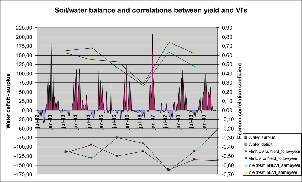
The lowest correlations occurred in 2006 (variation in VI’s 2006 vs. variation in Yield 2007), with Pearson coefficient of 0.29 for min EVI and of 0.27 for min NDVI, respectively, and this must have been caused by adverse weather conditions in 2006. Several factors can influence yield but water deficit is one of the most important [43]. According to the water balance for Guaxupé location (Figure 8), there was a long-drawn drought in 2006 that advanced during nine months until mid-November, which could have affected flowering development and, consequently, the relationship between coffee yield in 2007 and VI’s in 2006. For the analysis between coffee yield and vegetation indices that same year, the continuous drought did not seem to have influenced the correlations because, in this case, the relationship may have been based on other factors such as occurrence of diseases [24] and mechanical damage caused by harvesting [44].
In general the relationships between vegetation indices and yields the following years were inverse and higher than vegetation indices and yields the same year. The negative signs indicated that in the same year, yield can affect the vegetation indices, due to a higher incidence of diseases and also to greater damages caused by mechanical harvesting (both promote leaf fall), while in consecutive years vegetation indices represented the yield, since the branches formed in that year will be responsible for yield the following year.
4. Discussion
Although the correlation results were smaller than those found in studies with annual crops [11–15] and errors were high, the trends suggest a leaf area dependence in relation to coffee yield in the same year. Coffee is a perennial crop and takes two years to complete its phenological cycle, unlike most other crops, which complete their reproductive cycle in one year. Thus this crop represents a unique set of problems because it follows a biannual phenological cycle and exhibits high and low production in alternated years. This feature has been reported by several authors [26,27] as one important factor to be incorporated on agrometeorological models for estimating coffee yield. An effective tool to assess this pattern and estimate it in spatial domain could improve significantly coffee yield modeling.
Brunsell et al. [19] used lagged correlation analysis and deviations from the annual cycle to relate yield to accumulated deviations in fractional vegetation. MODIS vegetation indices were spatially aggregated over the municipally of Monte Santo de Minas, Minas Gerais, Brazil. The authors noted that data from MODIS vegetation indices converted into fractional vegetation indicate trends in coffee yield. Since the correlation between vegetation indices and yield is significant in our study, the alternated pattern in coffee yield is also true for vegetation indices. Thus, it is possible to infer the biennial effect through vegetation indices.
As shown in Tables 2–5, these trends can also be seen in the level of pixels vs. yield of coffee plot, especially for the amplitude and minimum values of VI.
The higher the coffee yield, the higher the defoliation levels, as suggested by positive correlations between VI variation range (ampEVI and ampNDVI) and variation in crop yield in the same year (Tables 2 and 3). Similar results were obtained by [44] in a field-based study where the authors found correlations around 0.90 between yield and crop defoliation in southern Minas Gerais region, Brazil. This defoliation could be attributed either to mechanical damage caused by harvest procedure or to a higher incidence of diseases such as coffee rust [20,21,24].
For the correlation analyses between VI and coffee yield the following year (Tables 4 and 5), the leaf biomass indicates trends in yield as an indirect result of increases in blooming. The water stress in 2007 could have affected blooming development and, consequently, the relationship between coffee yield that year and VI’s in 2006 (Figure 8). Since it is not possible to use passive remote sensing to quantify the magnitude of the coffee blooming in the study region because of the presence of clouds when coffee trees are flowering, leaf biomass is still a reasonable way to estimate coffee yield.
The better results obtained with the minimum values could point toward the most appropriate period in the study region for image acquisition to be used in further studies. When there are no clouds during this period (August/September) and if there are other images available with better spatial resolution as TM/Landsat, good results are also expected, since the main limitation of MODIS images in this case is their low spatial resolution.
In addition to the meteorological variables, the spectral response of coffee plantation can be influenced by pruning, plant spacing, intercropping system and others cultural practices. These factors can promote several uncertainties when vegetation index is correlated with productivity as shown by the high errors obtained. Moreover, even the best results of this analysis show that the vegetation indices can only explain about 50% of yield variance. In this way correlation analysis showed that vegetation indices did not entirely explain yield variation because there are a lot of factors responsible for final yield, but these indices could be useful as indicators of coffee biennial yield.
In relation to the vegetation indices evaluated, minEVI seems to be slightly better than minNDVI in our study, since in the analyzed period the correlations between minEVI values and yield were significant while the correlation between minNDVI values and yield were not significant in all analyzed years (Tables 2–5). A known limitation of NDVI index is the decrease or the saturation in sensitivity when leaf area index values (LAI) increase [45,46], such as coffee trees that can reach values of LAI higher than 8 [47]. Delalieux et al. [48] found the NDVI saturation effect when leaf area rates of crops exceed the value 5. On the other hand, EVI has shown to be less prone to saturation effect with higher sensitivity in regions of high biomass [49,50] which could make it more appropriate for studies of coffee canopy.
In our study we assessed correlations between metrics derived from MODIS vegetation indices and coffee yield. Only pixels overlapping large coffee plots were related to yield of the respective plots. The results point toward the possibility of using higher spatial resolution imagery to estimate the biennial bearing effect on coffee yield at the level of individual coffee fields. It can also be associated to agrometeorological models for estimating coffee yield in the spatial domain.
5. Conclusions
Among the five metrics derived from MODIS vegetation indices, including amplitude, sum, maximum, minimum and average values over the year, the minimum values were better correlated with coffee yield. Based on significance of correlation for every year and higher Pearson coefficients, correlation analysis between minimum values of vegetation indices (NDVI; EVI) and coffee yield the following year presented better results—Pearson coefficients ranging from 0.29 to 0.74 for minEVI and 0.27 to 0.68 for minNDVI, significant in both cases in five out of the six analyzed years. Even the best results of this analysis showed that the predictions are not high—Standard errors of prediction ranging from 0.42 to 0.61 for minEVI and 0.45 to 0.61 for minNDVI. The lowest correlations, that occurred in 2006 (variation in VI’s 2006 vs. variation in Yield 2007), with Pearson coefficient of 0.29 for minEVI and of 0.27 for minNDVI, have been caused by a long-drawn drought in 2006 which affected flowering development and, consequently, the relationship between coffee yield in 2007 and VI’s in 2006. Therefore, if no extreme weather event happens, minimum values of EVI and NDVI over the year were found to be useful as indicators of coffee biennial yield, since the trends properly reflect the coffee yield. Moreover, the best correlations were observed with vegetation index data obtained in August/September, the period in which there are cloud-free higher spatial resolution images, which can produce better results.
Despite the low spatial resolution of MODIS data and the fact that yield is a complex factor because it depends on several conditions, the indices were able to express the relationships between leaf biomass and coffee yield. Although coffee yield cannot be estimated exclusively from MODIS vegetation indices, these indices can be derived from higher spatial resolution images in order to obtain better results and can be used coupled with agrometeorogical models for estimating coffee yield.
Acknowledgments
To CNPq–Conselho Nacional de Desenvolvimento Científico e Tecnológico–“National Counsel of Technological and Scientific Development” for the research fellowship.
References
- Embrapa Café. Histórico. Available online: http://www22.sede.embrapa.br/cafe/unidade/historico.htm (accessed on 4 May 2009).
- Cordero-Sancho, S.; Sader, S.A. Spectral analyses and classification accuracy of coffee crops using Landsat and a topographic-environmental model. Int. J. Remote Sens 2007, 28, 1577–1593. [Google Scholar]
- Ramirez, G.M.; Zullo, J.J.; Assad, E.D.; Pinto, H.S. Comparison between Ikonos-II and Landsat/ETM+ satellites data in the study of coffee areas. Pesq. Agropec. Bras 2006, 41, 661–666. [Google Scholar]
- Moreira, M.A.; Adami, M.; Rudorff, B.F.T. Spectral and temporal behavior analysis of coffee crop in Landsat images. Pesq. Agropec. Bras 2004, 39, 223–231. [Google Scholar]
- Nagler, P.; Morino, K.; Murray, R.S.; Osterberg, J.; Glenn, E. An empirical algorithm for estimating agricultural and riparian evapotranspiration using MODIS enhanced vegetation index and ground measurements of ET. I. Description of method. Remote Sens 2009, 1, 1273–1297. [Google Scholar]
- Hatfield, J.L.; Prueger, J.H. Value of using different vegetative indices to quantify agricultural crop characteristics at different growth stages under varying management practices. Remote Sens 2010, 2, 562–578. [Google Scholar]
- Asner, G.P. Cloud cover in Landsat observations of the Brazilian Amazon. Int. J. Remote Sens 2001, 22, 3855–3862. [Google Scholar]
- Sano, E.E.; Ferreira, L.G.; Asner, G.P.; Steinke, E.T. Spatial and temporal probabilities of obtaining cloud-free Landsat images over the Brazilian tropical savanna. Int. J. Remote Sens 2007, 28, 2739–2752. [Google Scholar]
- Maxwell, S.K. Downscaling pesticide use data to the crop field level in California using landsat satellite imagery: Paraquat case study. Remote Sens 2011, 3, 1805–1816. [Google Scholar]
- Funk, C.; Budde, M.E. Phenologically-tuned MODIS NDVI-based production anomaly estimates for Zimbabwe. Remote Sens. Environ 2009, 113, 115–125. [Google Scholar]
- Mkhabela, M.S.; Bullock, P.; Raj, S.; Wang, S.; Yang, Y. Crop yield forecasting on the Canadian Prairies using MODIS NDVI data. Agr. For. Meteorol 2011, 151, 385–393. [Google Scholar]
- Becker-Reshef, I.; Vermote, E.; Lindeman, M.; Justice, C. A generalized regression-based model for forecasting winter wheat yields in Kansas and Ukraine using MODIS data. Remote Sens. Environ 2010, 114, 1312–1323. [Google Scholar]
- Ren, J.; Chen, Z.; Zhou, Q.; Tang, H. Regional yield estimation for winter wheat with MODIS-NDVI data in Shandong, China. Int. J. Appl. Earth Obs. Geoinf 2008, 10, 403–413. [Google Scholar]
- Panda, S.S.; Ames, D.P.; Panigrahi, S. Application of vegetation indices for agricultural crop yield prediction using neural network techniques. Remote Sens 2010, 2, 673–696. [Google Scholar]
- Laurila, H.; Karjalainen, M.; Kleemola, J.; Hyypä, J. Cereal yield modeling in Finland using optical and radar remote sensing. Remote Sens 2010, 2, 2185–2239. [Google Scholar]
- Ma, Y.; Wang, S.; Zhang, L.; Hou, Y.; Zhuang, L.; He, Y.; Wang, F. Monitoring winter wheat growth in North China by combining a crop model and remote sensing data. Int. J. Appl. Earth Obs. Geoinf 2008, 10, 426–437. [Google Scholar]
- Wolfe, R.E.; Roy, D.P.; Vermote, E.F. The MODIS land data storage, gridding and compositing methodology: L2 Grid. IEEE Trans. Geosci. Remote Sens 1998, 36, 1324–1338. [Google Scholar]
- Justice, C.; Townshend, J. Special issue on the moderate resolution imaging spectroradiometer (MODIS): A new generation of land surface monitoring. Remote Sens. Environ 2002, 83, 1–2. [Google Scholar]
- Brunsell, N.A.; Pontes, P.P.B.; Lamparelli, R.A.C. Remotely sensed phenology of coffee and its relationship to yield. GISci. Remote Sens 2009, 46, 289–304. [Google Scholar]
- Avelino, J.; Zelaya, H.; Merlo, A.; Pineda, A.; Ordoñez, M.; Savary, S. The intensity of a coffee rust epidemic is dependent on production situations. Ecol. Model 2006, 197, 431–447. [Google Scholar]
- Costa, M.J.N.; Zambolim, L.; Rodrigues, F.A. Effect of levels of coffee berry removals on the incidence of rust and on the level of nutrients, carbohydrates and reductor sugar. Fitopatol. Bras 2006, 31, 564–571. [Google Scholar]
- Chalfoun, S.M. Relationship of different indices of rust infection (Hemileia vastatrix Berk. & Br.) on the production of coffee (Coffea arabica L.) in some localities of the State of Minas Gerais. Fitopatol. Bras 1981, 6, 137–142. [Google Scholar]
- Eskes, A.B.; Carvalho, A. Variation for incomplete resistance to Hemileia vastatrix in Coffea Arábica. Euphytica 1983, 32, 625–637. [Google Scholar]
- Brown, J.S.; Whan, J.H.; Kenny, M.K.; Merriman, P.R. The effect of coffee leaf rust on foliation and yield of coffee in Papua New Guinea. Crop Prot 1995, 14, 589–592. [Google Scholar]
- Zambolim, L.; do Vale, F.X.R.; Costa, H.; Pereira, A.A.; Chaves, G.M. Epidemiology and Integrated Control of Coffee Rust. In The State of the Art Technology in the Production of Coffee; Zambolim, L., Ed.; UFV: Viçosa, MG, Brazil, 2002; pp. 369–450. [Google Scholar]
- Carvalho, L.G.; Sediyama, G.C.; Cecon, P.R.; Alves, H.M.R. Evaluation of an agrometeorological model to predict coffee productivity on three sites in southern Minas Gerais State, Brazil. Rev. Bras. Agrometeorol 2003, 11, 343–352. [Google Scholar]
- Picini, A.G.; Camargo, M.B.P.; Ortolani, A.A.; Fazuoli, L.C.; Bollergallo, P. Test and analysis of agrometeorological models for predicting coffee yield. Bragantia 1999, 58, 157–170. [Google Scholar]
- Camargo, A.P.; Camargo, M.B.P. Definition and outline for the phenological phases of arabic coffee under brazilian tropical conditions. Bragantia 2001, 60, 65–68. [Google Scholar]
- Huete, A.R.; Liu, H.Q.; Batchily, K.; van Leeuwen, W.J.D. A comparison of vegetation indices over a global set of TM images for EOS-MODIS. Remote Sens. Environ 1997, 59, 440–451. [Google Scholar]
- Liu, H.Q.; Huete, A. A feedback based modification of the NDVI to minimize canopy background and atmospheric noise. IEEE Trans. Geosci. Remote Sens. 1995, 33, 457–465. [Google Scholar]
- Huete, A.; Justice, C.; Liu, H. Development of vegetation and soil indices for MODIS-EOS. Remote Sens. Environ 1994, 49, 224–234. [Google Scholar]
- Rouse, J.W.; Haas, R.H.; Schell, J.A. Monitoring the Vernal Advancement and Retrogradation (Greenwave Effect) of Natural Vegetation; Texas A&M University: College Station, TX, USA, 1974. [Google Scholar]
- Moreira, M.A.; Rudorff, B.F.T.; Barros, M.A.; Faria, V.G.C.; Adami, M. Geotecnologies to map coffee fields in the states of minas gerais and são paulo. Agr. Eng 2010, 30, 1123–1135. [Google Scholar]
- Roy, D.P.; Ju, J.; Lewis, P.; Schaaf, C.; Gao, F.; Hansen, M.; Lindquist, E. Multi-temporal MODIS-Landsat data fusion for relative radiometric normalization, gap filling, and prediction of Landsat data. Remote Sens. Environ 2008, 112, 3112–3120. [Google Scholar]
- Câmara, G.; Souza, R.C.M.; Freitas, U.M.; Garrido, J.C.P. Spring: Integrating remote sensing and GIS with object-oriented data modelling. Comput. Graph 1996, 15, 13–22. [Google Scholar]
- Freitas, R.M.; Arai, E.; Adami, M.; Ferreira, A.F.; Sato, F.Y.; Shimabukuro, Y.E.; Rosa, R.R.; Anderson, L.O.; Rudorff, B.F.T. Virtual laboratory of remote sensing time series: visualization of MODIS EVI2 data set over South America. J. Comput. Interdiscipl. Sci 2011, 31, 57–68. [Google Scholar]
- Sakamoto, T.; van Nguyen, N.; Ohno, H.; Ishitsuka, N.; Yokozawa, M. Spatio-temporal distribution of rice phenology and cropping systems in the mekong delta with special reference to the seasonal water flow of the Mekong and Bassac rivers. Remote Sens. Environ 2006, 100, 1–16. [Google Scholar]
- Sakamoto, T.; Yokozawa, M.; Toritani, H.; Shibayama, M.; Ishitsuka, N.; Ohno, H. A crop phenology detection method using time-series MODIS data. Remote Sens. Environ 2005, 96, 366–374. [Google Scholar]
- Daubechies, I. Orthonormal bases of compactly supported wavelets. Commun. Pure Appl. Math 1988, 41, 909–996. [Google Scholar]
- Marsden, C.; le Maire, G.; Stape, J.-L.; Seen, D.L.; Roupsard, O.; Cabral, O.; Epron, D.; Lima, A.M.N.; Nouvellon, Y. Relating MODIS vegetation index time-series with structure, light absorption and stem production of fast-growing eucalyptus plantations. For. Ecol. Manag 2010, 259, 1741–1753. [Google Scholar]
- Kastens, J.H.; Kastens, T.L.; Kastens, D.L.A.; Price, K.P.; Martinko, E.A.; Lee, R.Y. Image masking for crop yield forecasting using AVHRR NDVI time series imagery. Remote Sens. Environ 2005, 99, 341–356. [Google Scholar]
- Damatta, F.M.; Ramalho, J.D.C. Impacts of drought and temperature stress on coffee physiology and production: A review. Braz. J. Plant Physiol 2006, 18, 55–81. [Google Scholar]
- Carr, M.K.V. The water relations and irrigation requirements of coffee. Exp. Agr 2001, 37, 1–36. [Google Scholar]
- Silva, F.M.D.; Alves, M.C.; Souza, J.C.S.; Oliveira, M.S. Effects of manual harvesting on coffee (coffea arabica L.) crop biannuality in Ijaci, Minas Gerais. Cienc. Agrotec 2010, 34, 625–632. [Google Scholar]
- Birky, A.K. NDVI and a simple model of deciduous forest seasonal dynamics. Ecol. Model 2001, 143, 43–58. [Google Scholar]
- Wang, Q.; Adiku, S.; Tenhunen, J.; Granier, A. On the relationship of NDVI with leaf area index in a deciduous forest site. Remote Sens. Environ 2005, 94, 244–255. [Google Scholar]
- Damatta, F.M.; Ronchi, C.P.; Maestry, M.; Barros, S.R. Ecophysiology of coffee growth and production. Braz. J. Plant Physiol 2007, 19, 485–510. [Google Scholar]
- Delalieux, S.; Somers, B.; Hereijgers, S.; Verstraeten, W.W.; Keulemans, W.; Coppin, P. A near infrared narrow-waveband ratio to determine Leaf Area Index in orchards. Remote Sens. Environ 2008, 112, 3762–3772. [Google Scholar]
- Boegh, E.; Soegaard, H.; Broge, N.; Hasager, C.B.; Jensen, N.O.; Schelde, K.; Thomsen, A. Airborne multispectral data for quantifying leaf area index, nitrogen concentration, and photosynthetic efficiency in agriculture. Remote Sens. Environ 2002, 8, 179–193. [Google Scholar]
- Huete, A.; Didan, K.; Muira, T.; Rodriguez, E.P.; Gao, X.; Ferrerra, L.G. Overview of the radiometric and biophysical performance of the MODIS vegetation indices. Remote Sens. Environ 2002, 83, 195–213. [Google Scholar]
Figure 1.
The study area in the south of Minas Gerais State.
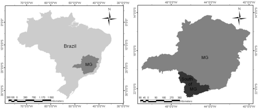
Figure 2.
Overlap of the limits of MODIS pixels with coffee fields in TM/Landsat 5 image, false color composite color 3B4R5G, (A) pixels fully occupied by coffee crop and (B) crop variability within a MODIS pixel in Landsat images.
Figure 2.
Overlap of the limits of MODIS pixels with coffee fields in TM/Landsat 5 image, false color composite color 3B4R5G, (A) pixels fully occupied by coffee crop and (B) crop variability within a MODIS pixel in Landsat images.
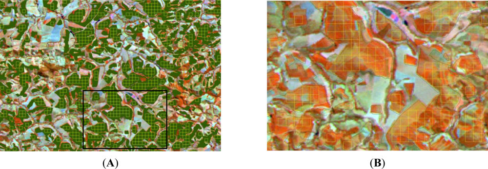
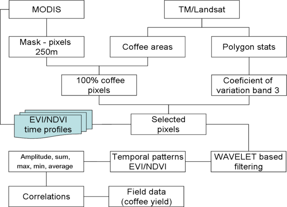
Figure 3.
Flowchart of data processing adopted in the study.

Figure 4.
Annual variation of vegetation indices for the selected pixels (A). Standard crop with the maximum vegetation index value for March (B) and minimum vegetation index for August (C) on Image TM/Landsat 3B4R5G.
Figure 4.
Annual variation of vegetation indices for the selected pixels (A). Standard crop with the maximum vegetation index value for March (B) and minimum vegetation index for August (C) on Image TM/Landsat 3B4R5G.
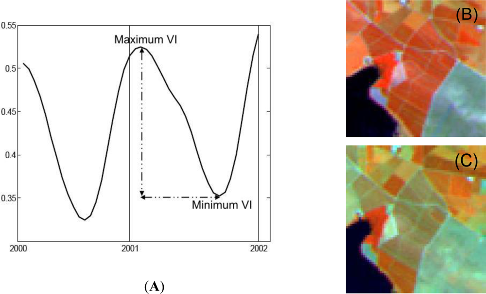
Figure 5.
Filtered EVI and NDVI time series for coffee crop and the original data (without filtering process).
Figure 5.
Filtered EVI and NDVI time series for coffee crop and the original data (without filtering process).
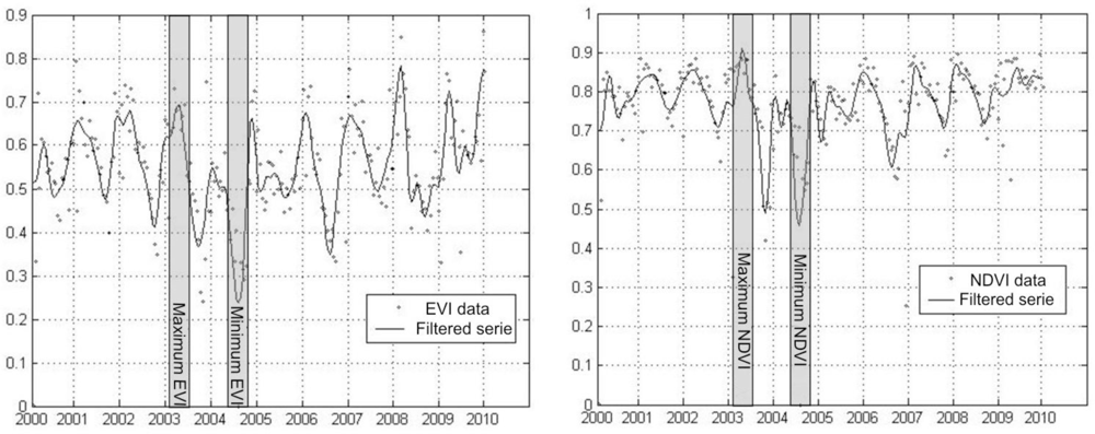
Figure 6.
Correlation between variation on coffee yield and variation on minimum values of vegetation indices (minEVI and minNDVI) for the same year.
Figure 6.
Correlation between variation on coffee yield and variation on minimum values of vegetation indices (minEVI and minNDVI) for the same year.
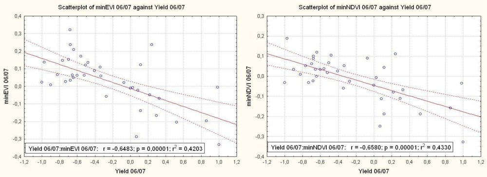
Figure 7.
Correlation between variation on minimum values of vegetation indices (minEVI and minNDVI) and variation on coffee yield the following year.
Figure 7.
Correlation between variation on minimum values of vegetation indices (minEVI and minNDVI) and variation on coffee yield the following year.
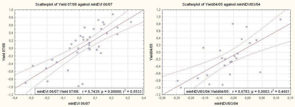
Figure 8.
Water balance for Guaxupé location and Pearson correlation coefficients from 2002 to 2009.
Figure 8.
Water balance for Guaxupé location and Pearson correlation coefficients from 2002 to 2009.


Table 1.
Number of yield data samples collected for each year (ni) and number of valid samples when we calculated the difference between 2 years (ni–ni−1).
| Table | 2002 | 2003 | 2004 | 2005 | 2006 | 2007 | 2008 | 2009 |
|---|---|---|---|---|---|---|---|---|
| ni | 20 | 25 | 27 | 32 | 37 | 37 | 37 | 35 |
| ni–ni−1 | - | 20 | 25 | 27 | 32 | 37 | 37 | 35 |
Table 2.
Correlation coefficients between variation on coffee yield and variation on EVI metrics in the same year for each metric assessed.
| Metric | 2002/03 | 2003/04 | 2004/05 | 2005/06 | 2006/07 | 2007/08 | 2008/09 | |
|---|---|---|---|---|---|---|---|---|
| N a | 20 | 25 | 27 | 32 | 37 | 37 | 35 | |
| ampEVI | r b | 0.56 | 0.50 | 0.48 | 0.32 | 0.40 | 0.20 | 0.41 |
| r-sq c | 0.32 | 0.25 | 0.23 | 0.10 | 0.16 | 0.04 | 0.17 | |
| p-value d | 0.01 | 0.01 | 0.01 | 0.07 | 0.01 | 0.23 | 0.01 | |
| SE e | 0.50 | 0.48 | 0.50 | 0.52 | 0.51 | 0.49 | 0.55 | |
| sumEVI | r b | −0.33 | 0.12 | −0.06 | −0.20 | −0.49 | −0.40 | −0.47 |
| r-sq c | 0.11 | 0.01 | 0.00 | 0.04 | 0.24 | 0.16 | 0.22 | |
| p-value d | 0.15 | 0.59 | 0.78 | 0.26 | <0.01 | 0.01 | <0.01 | |
| SE e | 0.57 | 0.55 | 0.57 | 0.53 | 0.48 | 0.46 | 0.53 | |
| maxEVI | r b | 0.29 | 0.34 | 0.24 | 0.12 | −0.05 | −0.15 | −0.10 |
| r-sq c | 0.08 | 0.11 | 0.06 | 0.01 | 0.00 | 0.02 | 0.01 | |
| p-value d | 0.22 | 0.11 | 0.22 | 0.53 | 0.78 | 0.38 | 0.56 | |
| SE e | 0.58 | 0.52 | 0.55 | 0.54 | 0.55 | 0.49 | 0.60 | |
| minEVI | r b | −0.46 | −0.38 | −0.50 | −0.45 | −0.65 | −0.54 | −0.55 |
| r-sq c | 0.21 | 0.14 | 0.25 | 0.20 | 0.42 | 0.30 | 0.31 | |
| p-value d | 0.04 | 0.07 | 0.01 | 0.01 | <0.01 | <0.01 | <0.01 | |
| SE e | 0.54 | 0.51 | 0.49 | 0.49 | 0.42 | 0.42 | 0.51 | |
| avrgEVI | r b | −0.33 | 0.12 | −0.06 | −0.20 | −0.49 | −0.40 | −0.47 |
| r-sq c | 0.11 | 0.01 | 0.00 | 0.04 | 0.24 | 0.16 | 0.22 | |
| p-value d | 0.15 | 0.59 | 0.78 | 0.26 | <0.01 | 0.01 | <0.01 | |
| SE e | 0.57 | 0.55 | 0.57 | 0.53 | 0.48 | 0.46 | 0.53 | |
asamples;
bpearson’s coefficient;
ccoefficient of determination;
dsignificance.;
estandard error
Table 3.
Correlation coefficients between variation on coffee yield and variation on NDVI metrics in the same year for each metric assessed.
| Metric | 2002/03 | 2003/04 | 2004/05 | 2005/06 | 2006/07 | 2007/08 | 2008/09 | ||
|---|---|---|---|---|---|---|---|---|---|
| N a | 20 | 25 | 27 | 32 | 37 | 37 | 35 | ||
| ampNDVI | r b | 0.44 | 0.33 | 0.10 | 0.41 | 0.42 | 0.26 | 0.11 | |
| r-sq c | 0.20 | 0.11 | 0.01 | 0.17 | 0.18 | 0.07 | 0.01 | ||
| p-value d | 0.05 | 0.11 | 0.61 | 0.02 | 0.01 | 0.12 | 0.52 | ||
| SE e | 0.54 | 0.52 | 0.57 | 0.50 | 0.50 | 0.48 | 0.60 | ||
| sumNDVI | r b | −0.15 | 0.25 | 0.10 | 0.07 | −0.36 | −0.40 | −0.23 | |
| r-sq c | 0.02 | 0.06 | 0.01 | 0.01 | 0.13 | 0.16 | 0.05 | ||
| p-value d | 0.52 | 0.23 | 0.61 | 0.69 | 0.03 | 0.01 | 0.18 | ||
| SE e | 0.60 | 0.54 | 0.57 | 0.54 | 0.51 | 0.46 | 0.59 | ||
| maxNDVI | r b | 0.11 | 0.07 | 0.07 | 0.37 | −0.20 | −0.30 | −0.19 | |
| r-sq c | 0.01 | 0.00 | 0.00 | 0.14 | 0.04 | 0.09 | 0.04 | ||
| p-value d | 0.64 | 0.75 | 0.73 | 0.03 | 0.23 | 0.07 | 0.28 | ||
| SE e | 0.60 | 0.55 | 0.57 | 0.51 | 0.54 | 0.48 | 0.60 | ||
| minNDVI | r b | −0.45 | −0.52 | −0.30 | −0.36 | −0.66 | −0.45 | −0.21 | |
| r-sq c | 0.20 | 0.27 | 0.09 | 0.13 | 0.43 | 0.20 | 0.04 | ||
| p-value d | 0.05 | 0.01 | 0.12 | 0.04 | <0.01 | <0.01 | 0.23 | ||
| SE e | 0.54 | 0.48 | 0.54 | 0.51 | 0.42 | 0.44 | 0.59 | ||
| avrgNDVI | r b | −0.15 | 0.25 | 0.10 | 0.07 | −0.36 | −0.40 | −0.23 | |
| r-sq c | 0.02 | 0.06 | 0.01 | 0.01 | 0.13 | 0.16 | 0.05 | ||
| p-value d | 0.52 | 0.23 | 0.61 | 0.69 | 0.03 | 0.01 | 0.18 | ||
| SE e | 0.60 | 0.54 | 0.57 | 0.54 | 0.51 | 0.46 | 0.59 | ||
asamples;
bpearson’s coefficient;
ccoefficient of determination;
dsignificance.;
estandard error.
Table 4.
Correlation coefficients between variation on EVI metrics and variation on coffee yield the following year for each metric assessed.
| Metric | 2002/03 | 2003/04 | 2004/05 | 2005/06 | 2006/07 | 2007/08 | |
|---|---|---|---|---|---|---|---|
| N a | 20 | 25 | 27 | 32 | 37 | 37 | |
| ampEVI | r b | −0.57 | −0.55 | −0.56 | −0.33 | −0.48 | −0.24 |
| r-sq c | 0.33 | 0.30 | 0.31 | 0.11 | 0.23 | 0.06 | |
| p-value d | 0.01 | 0.01 | <0.01 | 0.06 | <0.01 | 0.17 | |
| SE e | 0.61 | 0.51 | 0.57 | 0.55 | 0.55 | 0.45 | |
| sumEVI | r b | 0.52 | 0.06 | 0.10 | 0.18 | 0.49 | 0.47 |
| r-sq c | 0.27 | 0.00 | 0.01 | 0.03 | 0.24 | 0.22 | |
| p-value d | 0.02 | 0.79 | 0.61 | 0.31 | <0.01 | <0.01 | |
| SE e | 0.61 | 0.57 | 0.58 | 0.55 | 0.48 | 0.44 | |
| maxEVI | r b | −0.17 | −0.29 | −0.27 | −0.16 | 0.01 | 0.20 |
| r-sq c | 0.03 | 0.08 | 0.07 | 0.02 | 0.00 | 0.04 | |
| p-value d | 0.49 | 0.17 | 0.18 | 0.39 | 0.93 | 0.25 | |
| SE e | 0.61 | 0.57 | 0.59 | 0.55 | 0.54 | 0.48 | |
| minEVI | r b | 0.62 | 0.55 | 0.53 | 0.29 | 0.74 | 0.62 |
| r-sq c | 0.39 | 0.30 | 0.28 | 0.09 | 0.55 | 0.39 | |
| p-value d | <0.01 | 0.01 | <0.01 | 0.10 | <0.01 | <0.01 | |
| SE e | 0.61 | 0.48 | 0.57 | 0.55 | 0.46 | 0.42 | |
| avgEVI | r b | 0.52 | 0.06 | 0.10 | 0.18 | 0.49 | 0.47 |
| r-sq c | 0.27 | 0.00 | 0.01 | 0.03 | 0.24 | 0.22 | |
| p-value d | 0.02 | 0.79 | 0.61 | 0.31 | <0.01 | <0.01 | |
| SE e | 0.61 | 0.57 | 0.58 | 0.55 | 0.48 | 0.44 | |
asamples;
bpearson’s coefficient;
ccoefficient of determination;
dsignificance.;
estandard error.
Table 5.
Correlation coefficients between variation on NDVI metrics and variation on coffee yield the following year for each metric assessed.
| Metric | 2002/03 | 2003/04 | 2004/05 | 2005/06 | 2006/07 | 2007/08 | |
|---|---|---|---|---|---|---|---|
| N a | 20 | 25 | 27 | 32 | 37 | 37 | |
| ampNDVI | r b | −0.63 | −0.47 | −0.26 | −0.34 | −0.40 | −0.30 |
| r-sq c | 0.39 | 0.22 | 0.07 | 0.12 | 0.16 | 0.09 | |
| p-value d | <0.01 | 0.02 | 0.19 | 0.06 | 0.01 | 0.08 | |
| SE e | 0.59 | 0.48 | 0.57 | 0.54 | 0.52 | 0.47 | |
| sumNDVI | r b | 0.34 | 0.03 | −0.04 | −0.12 | 0.38 | 0.42 |
| r-sq c | 0.12 | 0.00 | 0.00 | 0.01 | 0.14 | 0.17 | |
| p-value d | 0.14 | 0.91 | 0.83 | 0.53 | 0.02 | 0.01 | |
| SE e | 0.60 | 0.55 | 0.59 | 0.54 | 0.50 | 0.48 | |
| maxNDVI | r b | 0.00 | −0.08 | −0.12 | −0.33 | 0.24 | 0.30 |
| r-sq c | 0.00 | 0.01 | 0.01 | 0.11 | 0.06 | 0.09 | |
| p-value d | 1.00 | 0.70 | 0.56 | 0.67 | 0.15 | 0.08 | |
| SE e | 0.60 | 0.52 | 0.59 | 0.55 | 0.53 | 0.48 | |
| minNDVI | r b | 0.65 | 0.68 | 0.46 | 0.27 | 0.63 | 0.48 |
| r-sq c | 0.43 | 0.46 | 0.21 | 0.07 | 0.39 | 0.23 | |
| p-value d | <0.01 | <0.01 | 0.02 | 0.14 | <0.01 | <0.01 | |
| SE e | 0.61 | 0.46 | 0.56 | 0.55 | 0.45 | 0.48 | |
| avgNDVI | r b | 0.34 | 0.03 | −0.04 | −0.12 | 0.38 | 0.42 |
| r-sq c | 0.12 | 0.00 | 0.00 | 0.01 | 0.14 | 0.17 | |
| p-value d | 0.14 | 0.91 | 0.83 | 0.53 | 0.02 | 0.01 | |
| SE e | 0.60 | 0.55 | 0.59 | 0.54 | 0.50 | 0.48 | |
asamples;
bpearson’s coefficient;
ccoefficient of determination;
dsignificance.;
estandard error.
Share and Cite
MDPI and ACS Style
Bernardes, T.; Moreira, M.A.; Adami, M.; Giarolla, A.; Rudorff, B.F.T. Monitoring Biennial Bearing Effect on Coffee Yield Using MODIS Remote Sensing Imagery. Remote Sens. 2012, 4, 2492-2509. https://doi.org/10.3390/rs4092492
AMA Style
Bernardes T, Moreira MA, Adami M, Giarolla A, Rudorff BFT. Monitoring Biennial Bearing Effect on Coffee Yield Using MODIS Remote Sensing Imagery. Remote Sensing. 2012; 4(9):2492-2509. https://doi.org/10.3390/rs4092492
Chicago/Turabian StyleBernardes, Tiago, Maurício Alves Moreira, Marcos Adami, Angélica Giarolla, and Bernardo Friedrich Theodor Rudorff. 2012. "Monitoring Biennial Bearing Effect on Coffee Yield Using MODIS Remote Sensing Imagery" Remote Sensing 4, no. 9: 2492-2509. https://doi.org/10.3390/rs4092492