With increased quality of synthetic aperture radar (SAR) systems utilizing polarimetric information recently, the development and applications of polarimetric SAR (POLSAR) are one of the current major topics in radar remote sensing. While conventional SAR systems handle only single polarimetric information, data acquired through POLSAR systems contain fully polarimetric information on the shift in polarization between the transmitted and received microwave. Thus, they have potential to increase further the ability of extracting physical quantities of the scattering targets. Therefore, they are used in broad fields of study such as visualization for classification [1,2], oil detection [3,4], and ship detection [5,6], to name a few.

Several decomposition techniques have been proposed along with the utilization of fully polarimetric data sets provided by POLSAR platforms. Most of them can be categorized into either of two main groups. One is based on eigenvalue analysis [7–9], and the other employs scattering model-based decomposition originally proposed by Freeman and Durden [10]. The basic idea behind this is that the backscattering power can be expressed as a linear sum of three different scattering power components.

The four-component scattering power decomposition (4-CSPD) [11,12] is one of the model-based decomposition methods, and it is an improved method of the previously devised three-component decomposition [10]. Using the 4-CSPD, one can decompose POLSAR data into four power categories: surface scattering power, double-bounce scattering power, volume scattering power, and helix scattering power. Many studies are being made in this field. For example, Zhang et al. [13] suggested a multiple-component scattering model (MCSM) by introducing an additional component that they call wire scattering. Some other studies incorporate an eigenvalue analysis into model-based decomposition [14–16] to correct for negative eigenvalues from the remainder covariance matrix after the volume contribution is subtracted.

According to [9,17], among all of the scattering components, double-bounce scattering occurs when the transmitted signal is reflected by ground/sea surfaces and man-made structures (or natural targets such as tree trunks). However, the problem appears for oblique urban blocks or man-made structures whose main scattering center is at an oblique direction with respect to the radar illumination [18]. In such areas, volume scattering (cross-polarized component) often becomes a major scattering process. Thus, output results from the decomposition analysis are sometimes confusing when classification such as urban and forested areas is made, because volume scattering comes from both areas. This makes the classification of man-made structures from other areas difficult. From the classification point of view, these two types of areas have quite different characteristics. Therefore, it would be better if these areas are separated more clearly.

To overcome this problem, the concept of rotation in the 4-CSPD has recently been proposed by Yamaguchi et al. [18]. They applied rotation to coherency matrices, so that cross-polarization (i.e., HV and VH) components, which are directly related to volume scattering, are suppressed, and double-bounce scattering increases instead. As a result, urban or industrial areas are successfully separated from forested areas more effectively.

In the present article, we introduce the 4-CSPD algorithm with rotation of covariance matrix and compare rotation of coherency and covariance matrices. This is because, although both approaches should yield a same result [19], detailed comparison has not yet been made and reported to date. Comparison is made among the 4-CSPD analyses with and without rotation of matrices. Examples are presented using ALOS-PALSAR (Advanced Land Observing Satellite-Phased Array L-band SAR) PLR (PoLaRimetric) data.

Since the detail of rotation of coherency matrix can be found in [18], we describe only rotation of covariance matrix, which should give the same results to the rotation of covariance matrix (although experimental verification has not yet been reported). The covariance matrix can be expressed as: (1) 〈 [ C ] 〉     =     [ 〈 | S H H | 2 〉 〈 2 S H H S H V * 〉 〈 S H H S V V * 〉 〈 2 S H V   S H H * 〉 〈 2 | S H V | 2 〉 〈 2 S H V S V V * 〉 〈 S V V   S H H * 〉 〈 2 S V V S H V * 〉 〈 | S V V | 2 〉 ] (2) =   [ C 11 C 12 C 13 C 21 C 22 C 23 C 31 C 32 C 33 ]where S_HH, S_HV, S_{V H} and S_{V V} denote the complex scattering elements at HH, HV, VH, and VV polarizations respectively, 〈〉 denotes the ensemble average of an arbitrary window size, and * denotes complex conjugate. The covariance matrix after rotation can be expressed using a unitary rotation matrix as: (3) [ C ( θ ) ]     =     [ U θ ] [ C ] [ U θ ] T (4) [ U θ ]     = 1 2   [ 1   +   cos 2 θ 2 sin   2 θ 1     −   cos   2 θ − 2 sin   2 θ 2   cos   2 θ 2 sin   2 θ 1   −   cos   2 θ − 2 sin   2 θ 1   +   cos   2 θ ]where T denotes matrix transpose, and θ denotes a rotation angle. The elements of the rotated covariance matrix are expressed as follows: (5) [ C ( θ ) ]     =     [ C 11 ( θ ) C 12 ( θ ) C 13 ( θ ) C 21 ( θ ) C 22 ( θ ) C 23 ( θ ) C 31 ( θ ) C 32 ( θ ) C 33 ( θ ) ] .where, using Equation (3), each element after rotation can be expressed in the same manner as in the rotation of coherency matrix, by replacing the elements of coherency matrix with those of covariance matrix. The important element is the cross-polarized term C₂₂(θ) given by (6) C 22 ( θ ) =     1 4 [ − C 11   +   2 Re ( C 13 )     +   ​ 2 C 22   −   C 33 ]   cos   4 θ   + ​ 2 2 Re ( C 12   −   C 23 ) sin   4 θ   +   ​     1 4 [ C 11   −   2 Re ( C 13 )   + C 22   + C 33 ] .

Now, we are going to minimize C₂₂(θ) because it is equivalent to minimizing volume scattering after the decomposition. Polarimetric matrices are rotated based on the angle which minimizes the cross-polarized component, so that the contribution of volume scattering power after the decomposition is suppressed. The derivative of C₂₂(θ) with respect to θ is (7) C 22 ′ ( θ )   =   ( C 11   −   2 Re ( C 13 )   −   2 C 22 ​ +   C 33 )   sin 4 θ   −   2 2 Re ( C 12   −   C 23 )   cos   4 θ .  

Therefore, when C′₂₂(θ) = 0, the angle is (8) tan   4 θ   =   2 2 Re ( C 12   −   C 23 ) C 11   −   2 Re ( C 13 )   −   2 C 22   +   C 33 . (9) θ   =   1 4   tan − 1 2 2 Re ( C 12   −   C 23 ) C 11   −   2 Re ( C 13 )   −   2 C 22   +   C 33 .

An extreme value can be derived from applying Equation (9) to Equation (6). It should be noted that arctan2 function, which many programming languages have, should be used to calculate Equation (9). Otherwise, the obtained angle may not minimize the cross-polarized component as it should be.

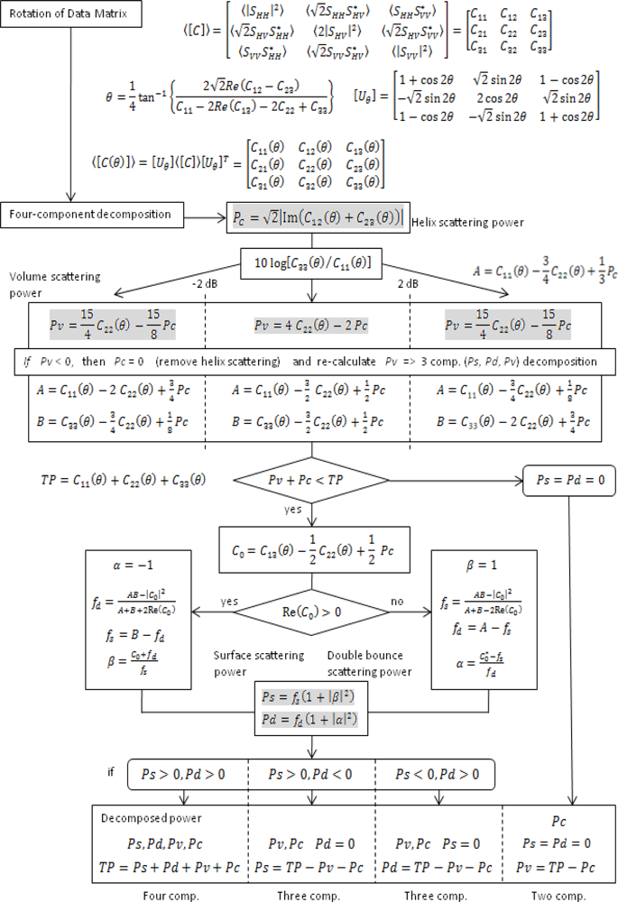
The algorithm of the 4-CSPD analysis using rotation of covariance matrix is summarized in this section. Figure 1 is the flowchart of the entire algorithm. First, a rotated covariance matrix [C(θ)] is created using the rotation angle described in the previous section. Next, the 4-CSPD algorithm is applied to the rotated covariance matrix [C(θ)] and the scattering powers are calculated. The helix scattering power Pc is derived first. Then, the volume scattering power Pv is calculated based on the value of (10) 10   log [ C 33 ( θ ) / C 11 ( θ ) ]

Once Pc and Pv are calculated, the surface scattering power Ps and the double-scattering power Pd can be determined by the remaining power (TP − Pc − Pv). If Pv + Pc > TP, the algorithm ends as two-component scattering power decomposition. The branch condition Re(C₀) > 0 is used for determining which scattering power, Ps or Pd, is dominant. C₀ can be defined in terms of the covariance matrix elements as: (11) C 0   =   C 13 ( θ )   −   1 2     C 22 ( θ )     +     1 2 P c .

As a result, all of the four scattering components are determined. If Ps or Pd becomes negative, it is substituted by zero and the other is determined by TP − Pc − Pv. It should also be noted that all of the four scattering components can be obtained directly from the rotated covariance matrix elements.

Since covariance matrix and coherency matrix are mutually interchangeable by unitary transformation, the output of this algorithm should exactly be the same as the output from the rotation of coherency matrix as long as the same angle, the one which optimally minimizes cross-polarized component, is chosen. This can easily be proven mathematically that both Equation (9) and (12) 2 θ     =     1 2 tan − 1 2 Re ( T 23 ) T 22   −   T 23 .from [18] have exactly the same form by assigning relevant scattering component into each equation. As for the equivalence between covariance and coherency matrix, it can also be shown mathematically that Pc and Pv have exactly the same form in both algorithms (covariance and coherency matrices) using the same manner as above. Thus, their equivalence is guaranteed. This equivalence applies to Equation (10) and Equation (11) as well. The contribution of remaining components, Ps and Pd, should also be identical in both matrices as stated in [19]. In order to confirm the equivalent nature between the 4-CSPD based on the covariance and coherence matrices, we provide the experimental results by both approaches in the following section.

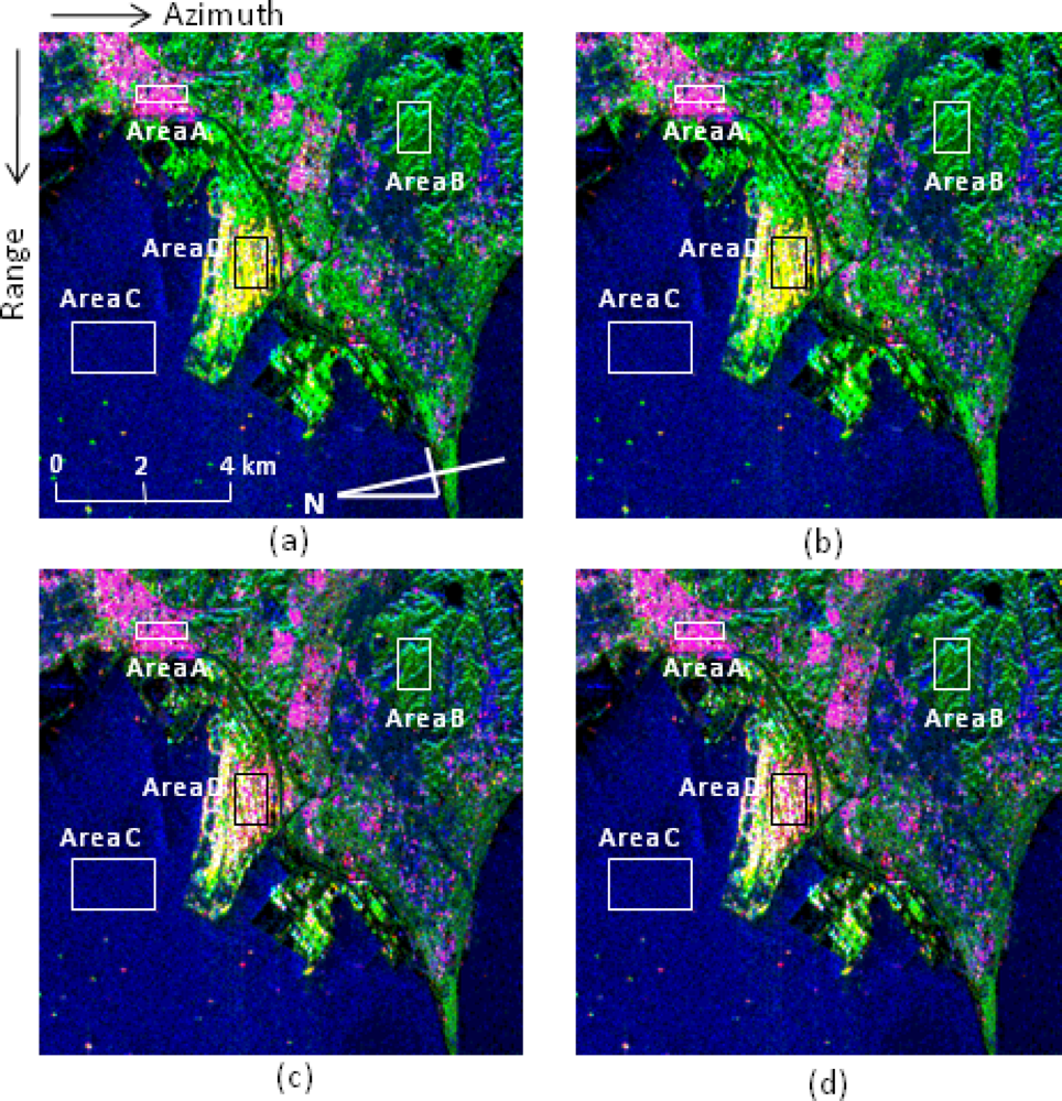
The algorithm is applied to ALOS-PALSAR data, and the results and discussions are presented in this section. Figure 2 shows parts of decomposed images of the Tokyo Bay and Futtsu Horn in Chiba Prefecture, Japan. The central coordinate is approximately at (139°52′E, 35°20′N), and the image size is about 11 km in both directions. The quad-polarization data used here were acquired by ALOS-PALSAR on 24 November 2008 (ALPSRP150972900-P1.1). In Figure 2, the left column shows the results from coherency matrix and the right column shows the results from covariance matrix. The upper row shows the decomposition images from conventional 4-CSPD and the lower row shows the decomposition images from 4-CSPD with rotation. The red, green, and blue colors represent double-bounce, volume, and surface scattering components respectively. There is no difference between the image from covariance matrix rotation and the image from coherency matrix rotation, as well as those without rotation. This result verifies that the rotation algorithm with covariance matrix agrees with the theoretical fact of unitary transformation.

The effect of the size of the moving window (i.e., ensemble average) has also been analyzed. As expected, if the size is too small, the result is too noisy and classification does not work very well. On the other hand, if the size is too large, the output becomes rougher and fine details are lost. An appropriate window size depends on each situation. Therefore, when the decomposition is performed, this should be taken into consideration. At this time, the ensemble average window size is 2 pixels in range direction and 16 pixels in azimuth direction.

Table 1 shows comparison of relative contribution of double-bounce, volume, surface, and helix scatterings to the total power before and after rotation, using the same region as in Figure 2. Only results from 4-CSPD with rotation of covariance matrix are shown in Table 1 because we confirmed that the results are precisely identical between coherency and covariance matrices. After rotation, volume scattering is suppressed and the contribution of double-bounce scattering becomes larger.

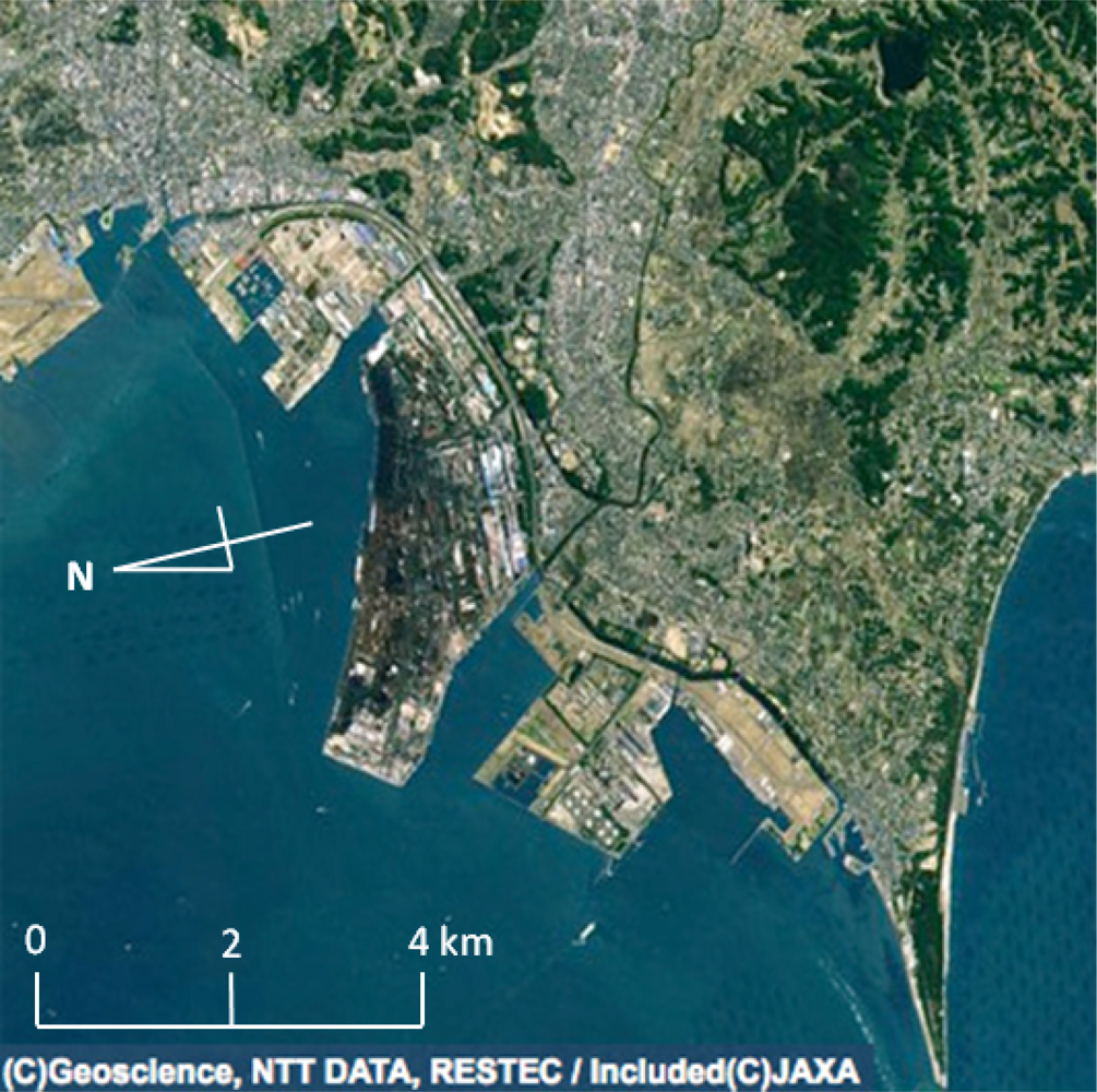
The central area in Figure 2 are classified as yellow in the upper images, but are classified as red in the lower images, increasing likelihood of being recognized as man-made structures. Figure 3 is an enlarged Google Earth image corresponding to the area in Figure 2. The red areas in the lower images in Figure 2 can be identified as industrialized bay areas in Figure 3, and the surface scattering areas represented in blue over land correspond to the rice paddies. After harvest in autumn these paddy fields are left as rough surfaces of bare soil. Some of the dots scattered on the sea surface turned into reddish from greenish after rotation and they are considered to be ships because they show strong Pd scattering and we know that there are no small islands in the area. Thus, the rotation method helps, by emphasizing Pd component, to classify backscattering on the sea not as rocks or tiny islands but as ships with more certainty.

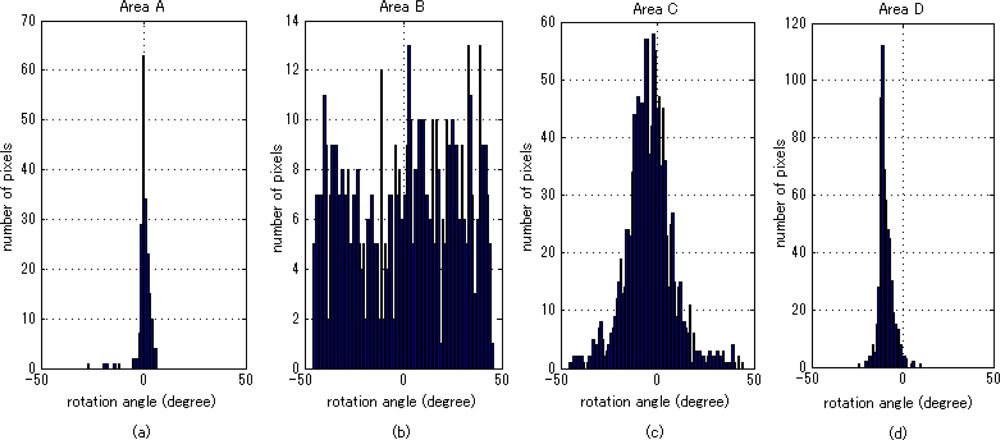
Figure 4 shows rotation angle distribution of selected areas in Figure 2. From left to right, the results from Areas A, B, C and D are shown respectively. Area A is a part of urban area and shows strong double-bounce scattering before applying rotation. Small rotation is observed in Area A. The possible explanation for this is that most urban structures are ideally facing the radar in a way that the double-bounce scattering is mostly observed. Thus, rotation is less necessary here. Area B is a part of mountainous area covered by forests and shows strong volume scattering. In Area B, rotation is randomly distributed across the entire range. Because the phases of cross-polarized components are randomly distributed, angles minimizing them are also randomly distributed. Area C is a part of sea area and mostly shows surface scattering. In Areas A and C, the center of rotation angle distribution is around zero. Finally, Area D is a part of industrial area which shows remarkable change after rotation. Here, the peak of angle shifts is around −10°, which is clearly different from other areas. It coincides with the fact that the structures in Area D are slightly tilted to the right in Figure 3.

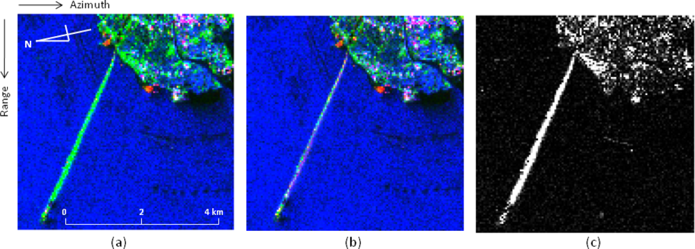
Figure 5 shows Tokyo Bay Aqua-Line (A highway across Tokyo Bay). The green color produced by the highway bridge in the left image turned into reddish in the middle image, highlighting enhanced double-bounce scattering, and Figure 5(c) clearly shows increase in double-bounce scattering between Figure 5(a,b). As a ground truth, we confirmed that the bridge does not have tall towers and large cables as described in the bridge analysis in [20] and there are many highway lamps and traffic and direction signs on the bridge. Thus, double-bounce scattering comes from the dihedral reflection between the surface of the bridge and them, and between the sea surface and the bridge. 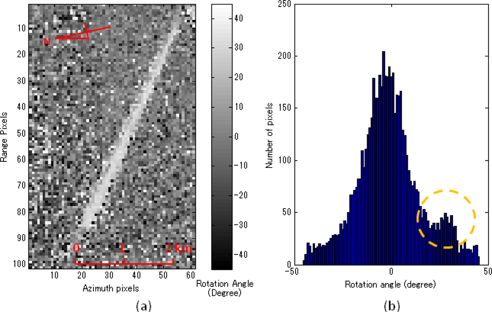Figure 6 shows rotation angle image and rotation angle distribution around the bridge. The peak around 30° in Figure 6(c) corresponds to the direction of the bridge from the radar illumination.

In this study, the four-component scattering power decomposition (4-CSPD) algorithm with rotation of covariance matrix is introduced. We demonstrated that the algorithm is correct by showing that the result of covariance matrix rotation is identical to that of coherency matrix rotation utilizing ALOS-PALSAR quad-polarization data. Although it is well known that the both matrices should produce the same result based on the theory of unitary transformation, experimental proof with rotation of the matrices has not been done before. We clarified that different types of areas react to the rotation algorithm differently. Urban or industrial areas showing strong double-bounce scattering with the original 4-CSPD (without rotation) are little affected by rotation. Forested areas show random distribution in rotation angles because of their randomness in polarization. Sea or smooth ground surface areas are moderately affected by rotation. Urban or industrial areas which have oblique structures to radar illumination show peaks of rotation angle distribution away from zero degree (center) unlike the other areas, and the degree seems to correspond to the angle between the radar illumination and the structures. We also showed that the rotation can improve the classification of man-made objects such as ships and bridges on the sea.