Optimal Exploitation of the Sentinel-2 Spectral Capabilities for Crop Leaf Area Index Mapping


Abstract
:
1. Introduction
2. Material and Methods
2.1. Test Site and Data Acquisition
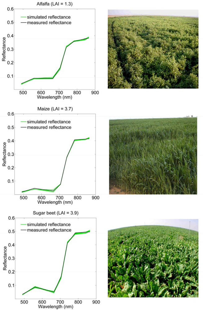
2.2. Relative Transfer (RT) Model and Inversion Procedures
2.3. Band Sensitivity Analysis
3. Results and Discussion
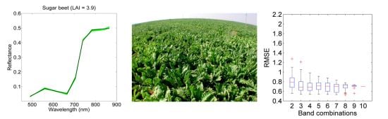
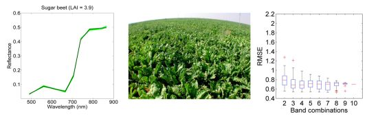
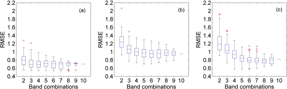
3.1. Optimal Number of Bands
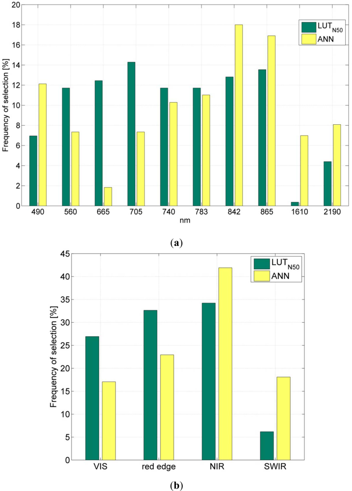
3.2. Optimal Spectral Sampling
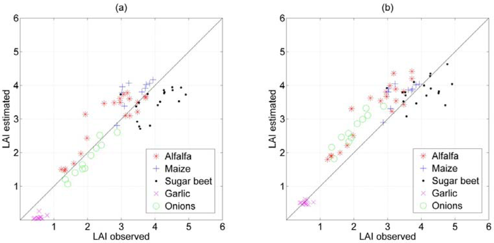
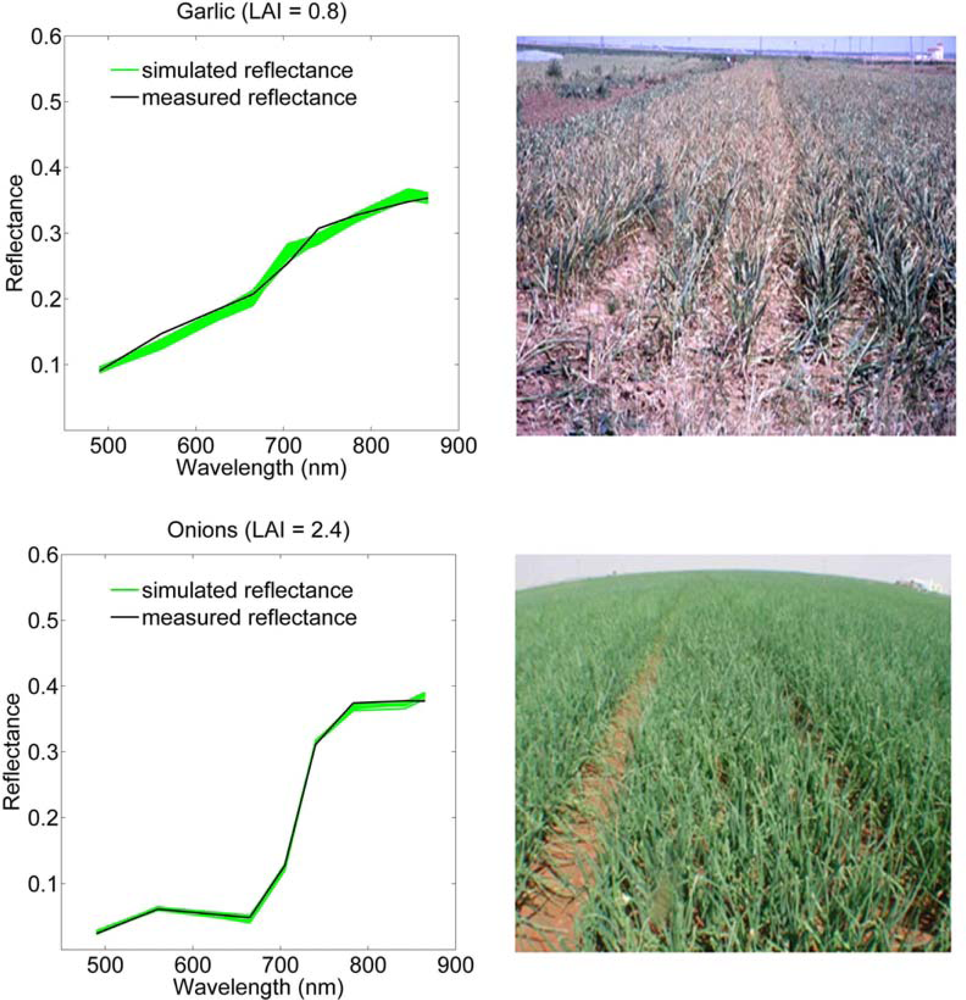
3.3. Crop Specific Differences
3.4. Limitations of the Study
4. Conclusions
Acknowledgments
References
- Baret, F.; Buis, S. Estimating canopy characteristics from remote sensing observations: Review of methods and associated problems. In Advances in Land Remote Sensing: System, Modeling, Inversion and Application; Liang, S., Ed.; Springer: Dordrecht, The Netherlands, 2008; pp. 173–201. [Google Scholar]
- Widlowski, J.L.; Pinty, B.; Gobron, N.; Verstraete, M.M.; Diner, D.J.; Davis, A.B. Canopy structure parameters derived from multi-angular remote sensing data for terrestrial carbon studies. Clim. Change 2004, 67, 403–415. [Google Scholar]
- Wolter, P.T.; Townsend, P.A.; Sturtevant, B.R. Estimation of forest structural parameters using 5 and 10 meter SPOT-5 satellite data. Remote Sens. Environ 2009, 113, 2019–2036. [Google Scholar]
- Potter, C.S.; Klooster, S.; Brooks, V. Interannual variability in terrestrial net primary production: Exploration of trends and controls on regional to global scales. Ecosystems 1999, 2, 36–48. [Google Scholar]
- D’Urso, G.; Richter, K.; Calera, A.; Osann, M.A.; Escadafal, R.; Garatuza-Pajan, J.; Hanich, L.; Perdigao, A.; Tapia, J.B.; Vuolo, F. Earth observation products for operational irrigation management in the context of the pleiades project. Agric. Water Manag 2010, 98, 271–282. [Google Scholar]
- Martimort, P.; Berger, M.; Carnicero, B.; Del Bello, U.; Fernandez, V.; Gascon, F.; Silvestrin, P.; Spoto, F.; Sy, O.; Arino, O.; et al. Sentinel-2: The optical high-resolution mission for GMES operational services. ESA Bulletin 2007, 131, 18–23. [Google Scholar]
- Drusch, M.; Gascon, F.; Berger, M. GMES Sentinel-2 Mission Requirements Document; European Space Agency, 2010; p. 42. http://esamultimedia.esa.int/docs/GMES/Sentinel-2_MRD.pdf (accessed date 02 February 2012).
- Dorigo, W.A.; Zurita-Milla, R.; de Wit, A.J.W.; Brazile, J.; Singh, R.; Schaepman, M.E. A review on reflective remote sensing and data assimilation techniques for enhanced agroecosystem modeling. Int. J. Appl. Earth Obs. Geoinf 2007, 9, 165–193. [Google Scholar]
- Baret, F.; Guyot, G. Potentials and limits of vegetation indices for LAI and apar assessment. Remote Sens. Environ 1991, 35, 161–173. [Google Scholar]
- Tucker, C.J. Red and photographic infrared linear combinations for monitoring vegetation. Remote Sens. Environ 1979, 8, 127–150. [Google Scholar]
- Glenn, E.; Huete, A.; Nagler, P.; Nelson, S. Relationship between remotely-sensed vegetation indices, canopy attributes and plant physiological processes: What vegetation indices can and cannot tell us about the landscape. Sensors 2008, 8, 2136–2160. [Google Scholar]
- Govaerts, Y.M.; Verstraete, M.M.; Pinty, B.; Gobron, N. Designing optimal spectral indices: A feasibility and proof of concept study. Int. J. Remote Sens 1999, 20, 1853–1873. [Google Scholar]
- Haboudane, D.; Miller, J.R.; Pattey, E.; Zarco-Tejada, P.J.; Strachan, I.B. Hyperspectral vegetation indices and novel algorithms for predicting green LAI of crop canopies: Modeling and validation in the context of precision agriculture. Remote Sens. Environ 2004, 90, 337–352. [Google Scholar]
- Hansen, P.M.; Schjoerring, J.K. Reflectance measurement of canopy biomass and nitrogen status in wheat crops using normalized difference vegetation indices and partial least squares regression. Remote Sens. Environ 2003, 86, 542–553. [Google Scholar]
- Atzberger, C.; Guerif, M.; Baret, F.; Werner, W. Comparative analysis of three chemometric techniques for the spectroradiometric assessment of canopy chlorophyll content in winter wheat. Comput. Electron. Agric 2010, 73, 165–173. [Google Scholar]
- Cho, M.A.; Skidmore, A.K.; Atzberger, C. Towards red-edge positions less sensitive to canopy biophysical parameters for leaf chlorophyll estimation using properties optique spectrales des feuilles (prospect) and scattering by arbitrarily inclined leaves (Sailh) simulated data. Int. J. Remote Sens 2008, 29, 2241–2255. [Google Scholar]
- Byambakhuu, I.; Sugita, M.; Matsushima, D. Spectral unmixing model to assess land cover fractions in mongolian steppe regions. Remote Sens. Environ 2010, 114, 2361–2372. [Google Scholar]
- Atkinson, P.M.; Tatnall, A.R.L. Introduction neural networks in remote sensing. Int. J. Remote Sens 1997, 18, 699–709. [Google Scholar]
- Camps Valls, G.; Bruzzone, L.; Rojo Álvarez, J.L.; Melgani, F. Robust support vector regression for biophysical variable estimation from remotely sensed images. IEEE Geosci. Remote Sens. Lett 2006, 3, 339–343. [Google Scholar]
- Baret, F.; Hagolle, O.; Geiger, B.; Bicheron, P.; Miras, B.; Huc, M.; Berthelot, B.; Nino, F.; Weiss, M.; Samain, O.; et al. LAI, FaPAR and fcover cyclopes global products derived from vegetation—Part 1: Principles of the algorithm. Remote Sens. Environ 2007, 110, 275–286. [Google Scholar]
- Jacquemoud, S.; Baret, F.; Andrieu, B.; Danson, F.M.; Jaggard, K. Extraction of vegetation biophysical parameters by inversion of the prospect plus sail models on sugar-beet canopy reflectance data - application to tm and aviris sensors. Remote Sens. Environ 1995, 52, 163–172. [Google Scholar]
- Koetz, B.; Baret, F.; Poilve, H.; Hill, J. Use of coupled canopy structure dynamic and radiative transfer models to estimate biophysical canopy characteristics. Remote Sens. Environ 2005, 95, 115–124. [Google Scholar]
- Goel, N.S. Models of vegetation canopy reflectance and their use in estimation of biophysical parameters from reflectance data. Remote Sens. Rev 1988, 4, 1–212. [Google Scholar]
- Combal, B.; Baret, F.; Weiss, M.; Trubuil, A.; Mace, D.; Pragnere, A.; Myneni, R.; Knyazikhin, Y.; Wang, L. Retrieval of canopy biophysical variables from bidirectional reflectance—Using prior information to solve the ill-posed inverse problem. Remote Sens. Environ 2003, 84, 1–15. [Google Scholar]
- Dorigo, W.; Richter, R.; Baret, F.; Bamler, R.; Wagner, W. Enhanced automated canopy characterization from hyperspectral data by a novel two step radiative transfer model inversion approach. Remote Sens 2009, 1, 1139–1170. [Google Scholar]
- Richter, K.; Atzberger, C.; Vuolo, F.; Weihs, P.; D'Urso, G. Experimental assessment of the Sentinel-2 band setting for rtm-based lai retrieval of sugar beet and maize. Can. J. Remote Sens 2009, 35, 230–247. [Google Scholar]
- Fang, H.L.; Liang, S.L.; Kuusk, A. Retrieving leaf area index using a genetic algorithm with a canopy radiative transfer model. Remote Sens. Environ 2003, 85, 257–270. [Google Scholar]
- Durbha, S.S.; King, R.L.; Younan, N.H. Support vector machines regression for retrieval of leaf area index from multiangle imaging spectroradiometer. Remote Sens. Environ 2007, 107, 348–361. [Google Scholar]
- Zhang, Q.Y.; Xiao, X.M.; Braswell, B.; Linder, E.; Baret, F.; Moore, B. Estimating light absorption by chlorophyll, leaf and canopy in a deciduous broadleaf forest using MODIS data and a radiative transfer model. Remote Sens. Environ 2005, 99, 357–371. [Google Scholar]
- Walthall, C.; Dulaney, W.; Anderson, M.; Norman, J.; Fang, H.L.; Liang, S.L. A comparison of empirical and neural network approaches for estimating corn and soybean leaf area index from Landsat ETM+ imagery. Remote Sens. Environ 2004, 92, 465–474. [Google Scholar]
- Atzberger, C.; Richter, K. Spatially constrained inversion of radiative transfer models for improved lai mapping from future Sentinel-2 imagery. Remote Sens. Environ 2011. accepted. [Google Scholar]
- Liang, S. Recent developments in estimating land surface biogeophysical variables from optical remote sensing. Progr. Phys. Geogr 2007, 31, 501–516. [Google Scholar]
- Delegido, J.; Verrelst, J.; Alonso, L.; Moreno, J. Evaluation of Sentinel-2 red-edge bands for empirical estimation of green lai and chlorophyll content. Sensors 2011, 11, 7063–7081. [Google Scholar]
- Atzberger, C.; Richter, K.; Vuolo, F.; Darvishzadeh, R.; Schlerf, M. Why confining to vegetation indices? Exploiting the potential of improved spectral observations using radiative transfer models. Proc. SPIE 2011, 8174, 81740Q. [Google Scholar]
- Darvishzadeh, R.; Skidmore, A.; Schlerf, M.; Atzberger, C. Inversion of a radiative transfer model for estimating vegetation lai and chlorophyll in a heterogeneous grassland. Remote Sens. Environ 2008, 112, 2592–2604. [Google Scholar]
- Meroni, M.; Colombo, R.; Panigada, C. Inversion of a radiative transfer model with hyperspectral observations for lai mapping in poplar plantations. Remote Sens. Environ 2004, 92, 195–206. [Google Scholar]
- Verger, A.; Baret, F.; Camacho, F. Optimal modalities for radiative transfer-neural network estimation of canopy biophysical characteristics: Evaluation over an agricultural area with chris/proba observations. Remote Sens. Environ 2011, 115, 415–426. [Google Scholar]
- Price, J. An approach for analysis of reflectance spectra. Remote Sens. Environ 1998, 64, 316–330. [Google Scholar]
- Thenkabail, P.S.; Enclona, E.A.; Ashton, M.S.; Van Der Meer, B. Accuracy assessments of hyperspectral waveband performance for vegetation analysis applications. Remote Sens. Environ 2004, 91, 354–376. [Google Scholar]
- Moreno, J.; Alonso, L.; Fernández, G.; Fortea, J.C.; Gandía, S.; Guanter, L. The Spectra Barrax Campaign (Sparc): Overview and First Results from CHRIS Data. Proceedings of 2nd CHRIS/PROBA Workshop, Frascati, Italy, 28–30 April 2004.
- Cocks, T.; Jenssen, R.; Stewart, A.; Wilson, I.; Shields, T. The Hymap Airborne Hyperspectral Sensor: The System, Calibration and Performance. Proceedings of 1rd EARSeL Workshop on Imaging Spectrometry, Zurich, Switzerland, 6–8 October 1998; pp. 37–42.
- Guanter, L.; Richter, R.; Moreno, J. Spectral calibration of hyperspectral imagery using atmospheric absorption features. Appl. Opt 2006, 45, 2360–2370. [Google Scholar]
- Welles, J.M.; Norman, J.M. Instrument for indirect measurement of canopy architecture. Agron. J 1991, 83, 818–825. [Google Scholar]
- Martinez, B.; Baret, F.; Camacho-de Coca, F.; Garcia-Haro, F.J.; Verger, A.; Melia, J. Validation of MSG vegetation products: Part I. Field retrieval of LAI and FVC from hemispherical photographs. Proc. SPIE 2004, 5568, 57–68. [Google Scholar]
- Martinez, B.; Cassiraga, E.; Camacho, F.; Garcia-Haro, J. Geostatistics for mapping leaf area index over a cropland landscape: Efficiency sampling assessment. Remote Sens 2010, 2, 2584–2606. [Google Scholar]
- Leblanc, S.G.; Chen, J.M.; Fernandes, R.; Deering, D.W.; Conley, A. Methodology comparison for canopy structure parameters extraction from digital hemispherical photography in boreal forests. Agric. For. Meteorol 2005, 129, 187–207. [Google Scholar]
- Ryu, Y.; Nilson, T.; Kobayashi, H.; Sonnentag, O.; Law, B.E.; Baldocchi, D.D. On the correct estimation of effective leaf area index: Does it reveal information on clumping effects? Agric. For. Meteorol 2010, 150, 463–472. [Google Scholar]
- Garrigues, S.; Shabanov, N.V.; Swanson, K.; Morisette, J.T.; Baret, F.; Myneni, R.B. Intercomparison and sensitivity analysis of leaf area index retrievals from LAI-2000, accupar, and digital hemispherical photography over croplands. Agric. For. Meteorol 2008, 148, 1193–1209. [Google Scholar]
- Soudani, K.; Francois, C.; le Maire, G.; Le Dantec, V.; Dufrene, E. Comparative analysis of IKONOS, SPOT, and ETM+ data for leaf area index estimation in temperate coniferous and deciduous forest stands. Remote Sens. Environ 2006, 102, 161–175. [Google Scholar] [Green Version]
- Feret, J.-B.; Francois, C.; Asner, G.P.; Gitelson, A.A.; Martin, R.E.; Bidel, L.P.R.; Ustin, S.L.; le Maire, G.; Jacquemoud, S. Prospect-4 and 5: Advances in the leaf optical properties model separating photosynthetic pigments. Remote Sens. Environ 2008, 112, 3030–3043. [Google Scholar]
- Verhoef, W. Light scattering by leaf layers with application to canopy reflectance modeling: The scattering by arbitrarily inclined leaves (sail) model. Remote Sens. Environ 1984, 16, 125–141. [Google Scholar]
- Jacquemoud, S.; Verhoef, W.; Baret, F.; Bacour, C.; Zarco-Tejada, P.J.; Asner, G.P.; Francois, C.; Ustin, S.L. Prospect plus sail models: A review of use for vegetation characterization. Remote Sens. Environ 2009, 113, S56–S66. [Google Scholar]
- Kuusk, A. The hot spot effect in plant canopy reflectance. In Photon and Vegetation Interactions; Myneni, R.B., Ross, J., Eds.; Springer-Verlag: Berlin, Germany, 1991; pp. 140–159. [Google Scholar]
- Jones, H.G.; Vaughan, R.A. Remote Sensing of Vegetation: Principles, Techniques and Applications; Oxford University Press: Oxford, UK, 2010. [Google Scholar]
- Schlerf, M.; Atzberger, C. Inversion of a forest reflectance model to estimate structural canopy variables from hyperspectral remote sensing data. Remote Sens. Environ 2006, 100, 281–294. [Google Scholar]
- Richter, K.; Vuolo, F.; D’Urso, G.; Palladino, M. Evaluation of near-surface soil water status through the inversion of soil-canopy radiative transfer models in the reflective optical domain. Int. J. Remote Sens 2012, in press. [Google Scholar]
- Dorigo, W.A. Improving the robustness of cotton status characterisation by radiative transfer model inversion of multi-angular chris/proba data. IEEE J. Sel. Top. Appl. Earth Obs. Remote Sens 2011, 1–12. [Google Scholar]
- Weiss, M.; Baret, F.; Myneni, R.B.; Pragnere, A.; Knyazikhin, Y. Investigation of a model inversion technique to estimate canopy biophysical variables from spectral and directional reflectance data. Agronomie 2000, 20, 3–22. [Google Scholar]
- Fourty, T.; Baret, F. Vegetation water and dry matter contents estimated from top-of-the-atmosphere reflectance data: A simulation study. Remote Sens. Environ 1997, 61, 34–45. [Google Scholar]
- Gausman, H.W.; Allen, W.A.; Cardenas, R. Reflectance of cotton leaves and their structure. Remote Sens. Environ 1969, 1, 19–22. [Google Scholar]
- Darvishzadeh, R.; Atzberger, C.; Skidmore, A.K.; Abkar, A.A. Leaf area index derivation from hyperspectral vegetation indices and the red edge position. Int. J. Remote Sens 2009, 30, 6199–6218. [Google Scholar]
- Brown, L.; Chen, J.M.; Leblanc, S.G.; Cihlar, J. A shortwave infrared modification to the simple ratio for lai retrieval in boreal forests: An image and model analysis. Remote Sens. Environ 2000, 71, 16–25. [Google Scholar]
- Khanna, S.; Palacios-Orueta, A.; Whiting, M.L.; Ustin, S.L.; Riaño, D.; Litago, J. Development of angle indexes for soil moisture estimation, dry matter detection and land-cover discrimination. Remote Sens. Environ 2007, 109, 154–165. [Google Scholar]
- Richter, K.; Hank, T.B.; Atzberger, C.; Mauser, W. Goodness-of-fit measures: What do they tell about vegetation variable retrieval performance from earth observation data. Proc. SPIE 2011, 8174, 81740R. [Google Scholar]
- Nash, J.E.; Sutcliffe, J.V. River flow forecasting through conceptual models Part I—A discussion of principles. J. Hydrol 1970, 10, 282–290. [Google Scholar]
- Archibald, R.; Fann, G. Feature selection and classification of hyperspectral images with support vector machines. IEEE Geosci. Remote Sens. Lett 2007, 4, 674–677. [Google Scholar]
- Baret, F. Biophysical Vegetation Variables Retrieval from Remote Sensing Observations. Proceedings of Remote Sensing for Agriculture, Ecosystems, and Hydrology XII, Toulouse, France, 20–22 September 2010; Neale, C.M.U., Maltese, A., Eds.; SPIE: Bellingham, WA, USA, 2010; 7824, pp. xvii–xix, front matter. [Google Scholar]
- Lauvernet, C.; Baret, F.; Hascoet, L.; Buis, S.; Le Dimet, F.-X. Multitemporal-patch ensemble inversion of coupled surface-atmosphere radiative transfer models for land surface characterization. Remote Sens. Environ 2008, 112, 851–861. [Google Scholar]
- Bach, H.; Mauser, W. Methods and examples for remote sensing data assimilation in land surface process modeling. IEEE Trans. Geosci. Remote Sens 2003, 41, 1629–1637. [Google Scholar]


| Variable | N class | Mean | Min | Max | SD |
|---|---|---|---|---|---|
| Leaf Model: PROSPECT-5 | |||||
| Cab1 [μg/cm2] | 4 | 45 | 20 | 90 | 30 |
| Cw2 [cm] | 4 | 0.01 | 0.001 | 0.1 | 0.01 |
| Cm1,2 [g/cm2] | 4 | 0.0075 | 0.002 | 0.02 | 0.0075 |
| Car3 [μg/cm2] | 2 | 10 | 0 | 25 | 15 |
| N1,2 | 4 | 1.5 | 1.0 | 2.5 | 1.0 |
| Canopy Model: SAIL | |||||
| LAI1,3 [m2/m2] | 6 | 2 | 0 | 6 | 2 |
| ALA1,3 [°] | 4 | 60 | 30 | 80 | 20 |
| Hot1,3 | 1 | 0.1 | 0.001 | 1 | 0.3 |
| αsoil5 | 4 | 1 | 0.6 | 1.4 | 0.5 |
| Arrangement (No. of Included Spectral Bands) | N (No. of Band Combinations) | RMSEmin | ||
|---|---|---|---|---|
| LUTN50 | LUTN1 | ANN | ||
| 2 | 45 | 0.56 | 0.93 | 0.91 |
| 3 | 120 | 0.54 | 0.77 | 0.73 |
| 4 | 210 | 0.54 | 0.73 | 0.58 |
| 5 | 252 | 0.54 | 0.70 | 0.58 |
| 6 | 210 | 0.54 | 0.70 | 0.58 |
| 7 | 120 | 0.53 | 0.73 | 0.59 |
| 8 | 45 | 0.53 | 0.77 | 0.64 |
| 9 | 10 | 0.56 | 0.78 | 0.67 |
| 10 | 1 | 0.70 | 0.95 | 0.84 |
| Crop Type | N | Range (Observed) | LUTN50: ‘Best Band’ Combination (8 Bands) | ANN: ‘Best Band’ Combination (5 Bands) | ||||||
|---|---|---|---|---|---|---|---|---|---|---|
| R2 | RMSE | NRMSE | NSE | R2 | RMSE | NRMSE | NSE | |||
| alfalfa | 20 | 1.22–3.72 | 0.80 | 0.50 | 0.20 | 0.63 | 0.84 | 0.71 | 0.28 | 0.26 |
| maize | 10 | 2.87–3.94 | 0.44 | 0.50 | 0.47 | −0.75 | 0.39 | 0.47 | 0.44 | −0.56 |
| sugar beet | 18 | 2.98–4.91 | 0.3 | 0.71 | 0.37 | −0.79 | 0.13 | 0.55 | 0.29 | −0.08 |
| garlic | 11 | 0.43–0.80 | 0.11 | 0.49 | 1.23 | −21.35 | 0.01 | 0.12 | 0.30 | −0.34 |
| onions | 11 | 1.34–2.88 | 0.92 | 0.25 | 0.16 | 0.68 | 0.88 | 0.70 | 0.45 | −1.51 |
| all crops | 70 | 0.43–4.91 | 0.86 | 0.53 | 0.12 | 0.83 | 0.85 | 0.58 | 0.13 | 0.80 |
Share and Cite
Richter, K.; Hank, T.B.; Vuolo, F.; Mauser, W.; D’Urso, G. Optimal Exploitation of the Sentinel-2 Spectral Capabilities for Crop Leaf Area Index Mapping. Remote Sens. 2012, 4, 561-582. https://doi.org/10.3390/rs4030561
Richter K, Hank TB, Vuolo F, Mauser W, D’Urso G. Optimal Exploitation of the Sentinel-2 Spectral Capabilities for Crop Leaf Area Index Mapping. Remote Sensing. 2012; 4(3):561-582. https://doi.org/10.3390/rs4030561
Chicago/Turabian StyleRichter, Katja, Tobias B. Hank, Francesco Vuolo, Wolfram Mauser, and Guido D’Urso. 2012. "Optimal Exploitation of the Sentinel-2 Spectral Capabilities for Crop Leaf Area Index Mapping" Remote Sensing 4, no. 3: 561-582. https://doi.org/10.3390/rs4030561