Article

Utilizing a Multi-Source Forest Inventory Technique, MODIS Data and Landsat TM Images in the Production of Forest Cover and Volume Maps for the Terai Physiographic Zone in Nepal

1
Finnish Forest Research Institute, Joensuu Unit, P.O. Box 68, FI-80101 Joensuu, Finland
2
Department of Forest Research and Survey, G.P.O. 3339, Babarmahal, Kathmandu, Nepal
*
Author to whom correspondence should be addressed.
Remote Sens. 2012, 4(12), 3920-3947; https://doi.org/10.3390/rs4123920
Submission received: 15 October 2012 / Revised: 4 December 2012 / Accepted: 5 December 2012 / Published: 10 December 2012

Abstract

:
An approach based on the nearest neighbors techniques is presented for producing thematic maps of forest cover (forest/non-forest) and total stand volume for the Terai region in southern Nepal. To create the forest cover map, we used a combination of Landsat TM satellite data and visual interpretation data, i.e., a sample grid of visual interpretation plots for which we obtained the land use classification according to the FAO standard. These visual interpretation plots together with the field plots for volume mapping originate from an operative forest inventory project, i.e., the Forest Resource Assessment of Nepal (FRA Nepal) project. The field plots were also used in checking the classification accuracy. MODIS satellite data were used as a reference in a local correction approach conducted for the relative calibration of Landsat TM images. This study applied a non-parametric k-nearest neighbor technique (k-NN) to the forest cover and volume mapping. A tree height prediction approach based on a nonlinear, mixed-effects (NLME) modeling procedure is presented in the Appendix. The MODIS image data performed well as reference data for the calibration approach applied to make the Landsat image mosaic. The agreement between the forest cover map and the field observed values of forest cover was substantial in Western Terai (KHAT 0.745) and strong in Eastern Terai (KHAT 0.825). The forest cover and volume maps that were estimated using the k-NN method and the inventory data from the FRA Nepal project are already appropriate and valuable data for research purposes and for the planning of forthcoming forest inventories. Adaptation of the methods and techniques was carried out using Open Source software tools.

1. Introduction

A general aim of forest inventory projects is to form a basis for decision-making and sustainable use of forest resources in the form of objective statistics at the national and regional levels and for administrative units. Conventionally, the statistics are obtained for pre-defined areas for the species-specific measures of the total volume of living and dead trees and merchantable volume characteristics. Questions and issues raised by the United Nations Framework Convention on Climate Change (UNFCCC) through its “Reducing Emissions from Deforestation and Forest Degradation” (REDD) program have increased the need for forest resource inventories and widened the application of their results. Countries already having suitable national forest inventory (NFI) frameworks can harness their NFIs to support also the assessment of green house gas (GHG) emissions. When developing countries, such as Nepal, for instance, are addressing this kind of task, technical and methodological support provided for assessing the forest resources may become even more important than before [1]. Due to the repetition requirements and temporal and geographical consistency conditions, the possibilities for utilizing remote sensing technology together with field inventory data are increasingly gaining the interest of the organizations responsible for the forest inventory activities related to the REDD mechanism (e.g., [2,3]). The operative inventory project “Forest Resource Assessment of Nepal” (FRA Nepal) belongs to the Finnish Government’s development aid toolkit. The FRA Nepal project is an example of an action that aims to develop cost-efficient inventory techniques based on information obtained from both conventional field inventories and remote sensing materials.
Biometrical modeling is also needed for inventory calculations that make use of remote sensing: for example, the calculation system for the FRA Nepal project consists of models for height or volume by tree species, which are necessary for imputing the values missing from the field data. Obtaining data from the tree level to the stand or plot level, or to the regional, level is a process by which inventory calculations and reporting modules are developed. To put all of this together, a forest inventory database is needed.
To combine field sample plot observations, digital map data and satellite image data, for classification or prediction purposes, multi-source forest inventory (MSFI) techniques have been developed [4,5]. Even if the pure inventory results are directly derived from the characteristics measured by the field sample plots, a multi-source approach aiming at the wall-to-wall mapping of forest characteristics requires remote sensing data. The necessary input data, i.e., the ground-truth data, comes from the inventory calculation system and from the Forest Inventory Database. Tools for processing GIS and image data are further utilized, for example, when classifying satellite image pixels and performing overlaying analysis.
A representative and large enough field sample for MSFI is a prerequisite, so that the estimation results are of a satisfactory quality and accurate enough. However, if only a small or very sparse sample of field plots is available, it must be possible to not only utilize plots on the same image, but also on neighboring images. For the FRA Nepal project, at minimum, it would be necessary to have a relative calibration procedure that would make it possible to combine several satellite images with respect to the target inventory areas. In our study case in Terai region, the main factors affecting the availability and the usability of Landsat TM images are cloudiness and seasonal variations. If cloud-free images are available, one alternative for relative calibration is then to adjust the radiometric properties of a subject image to those of a reference image [611]. Seasonal variation effects between images can partly be decreased by aiming to use images from the same time of year [6]. For tackling the problems caused by cloudiness, gap-filling approaches have been presented, where several images are used to cover the gaps in a selected image [12].
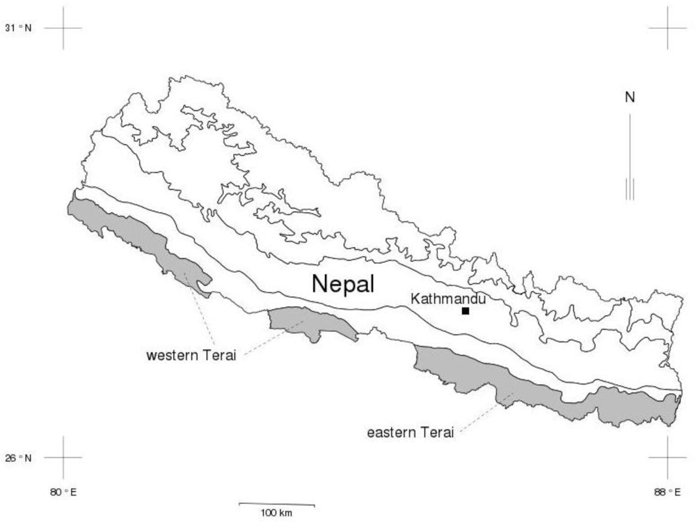
The aim of this study was to produce thematic maps of forest cover (forest/non-forest) and total stand volume for the Terai region in southern Nepal using a non-parametric, k-nearest neighbor technique. The pre-processing of Landsat TM images was conducted by using MODIS satellite data as a reference in a local correction approach. Mixed modeling was utilized for the generalization of sample tree characteristics that was conducted as a part of calculating the stand volumes by sample plots (see Appendix). The approach used to create the forest cover map was based on a combination of Landsat TM satellite data and visual interpretation data, i.e., a sample grid of visual interpretation plots by which we obtained the land use classification according to the FAO standard. For the volume mapping procedure, we utilized Landsat TM data, the forest cover map and the total stand volumes obtained by the field measured sample plots.

2. Materials

2.1. Study Area

The target area of the study, i.e., the Terai region, is located approximately between 26°15′–29°15′N and 80°00′–88°15′E. The Terai region is the southernmost of the five physiographic zones of Nepal and comprises 14% of the country’s land (Figure 1). In contrast to the other four physiographic zones, the terrain in this subtropical lowland plateau is topographically less complex, and its elevation varies from 60 to 330 m above sea level [13]. In this study, the western Terai comprises the two leftmost sub-regions of Terai, whereas the eastern Terai consists only of the rightmost sub-region of Terai (Figure 1).

2.2. Image Materials

Three Landsat TM satellite images from the western part of Terai and four images from the eastern part of Terai were included in two image mosaics, one covering western Terai in the UTM zone of 44 and another covering eastern Terai in the UTM zone of 45 (Table 1).
MODIS surface reflectance products provide an estimate of the surface spectral reflectance as it would be measured at ground level in the absence of atmospheric scattering or absorption. The MODIS Surface Reflectance product “MYD09A1” is a combination of the best possible observations in an eight-day time period at a 500-m resolution at the sinusoidal projection [14].
MYD09A1 material from the h25v06 and h24v06 sinusoidal tiles were utilized as image mosaic reference materials. The eight-day time interval of both MODIS products was from 10 February 2010 to 17 February 2010. The MODIS’s data coverage could be found from a time interval close to the dates for the Landsat images, which provided a quite reasonable starting point for image mosaic building and image interpretation purposes. One Landsat TM image from the north-western side of Terai was taken in 2011, thus representing a difference of just one year from the time-point of the MODIS data.
The MODIS Reprojection Tool [15] was used to transform the MODIS data into a UTM zone44 and zone45 coordinate system with wgs84 datum and 500-m resolution. All other image processing operations were carried out using Open Source tools and the utilities of GDAL, Quantum GIS and GRASS GIS [1618].

2.3. Two-Phase Sampling and Visual Interpretation Data

The setup of the ongoing national forest inventory was designed for the FRA Nepal project and formed the basis for this study. In the FRA Nepal project, a stratified systematic cluster sampling design with a two-phase cluster sampling method was applied [19,20].
In order to locate the sampling units, i.e., the sample plots within square clusters, throughout the whole country, a 4 km by 4 km grid was created. Each cluster consisted of six sample plots in two parallel lines in a North-South direction; the sample plots were 150 m apart and the distance between the North-South lines was 300 m (see Figure 2(a)). The sampling of clusters with the sample plots for the field measurements was conducted in two phases [20]. During the first phase, each cluster of six plots along the 4 km by 4 km grid covering the entire country was visually classified according to land use class (1 = Forest area (n = 1,603), 2 = Other wooded area (n = 131), 3 = Agricultural area with tree cover (n = 796), 4 = Agricultural area without tree cover (n = 4,168), 5 = Built-up area with tree cover (n = 202), 6 = Built-up area without tree cover (n = 119), 7 = Roads (n = 3), 8 = Other area (n = 229), 9 = Water area (n = 282), where n is the number of observations in Terai) and accessibility. Technically, the interpretation was implemented using Google Earth, a virtual globe and satellite imagery viewer [21] consisting of freely available satellite images and additional data layers, including RapidEye imagery, topographical maps and the sampling grid for Nepal. In this study, the visual interpretation data for the Terai physiographic zone comprised altogether 7,533 plotwise observations within 1,281 clusters. During the second phase, the selection of clusters for field measurements was done by strata. The first stratum contained the clusters having at least one plot in the forest area and the second stratum contained the clusters with no forest area plots in the 1st phase sample. During this sampling process, more weight was given to the clusters comprising plots on forest area. Only the four-corner plots of the cluster in a square with a side length of 300 m were used in these analyses (see Figure 2(a)).

2.4. Field Data

The field data for this study were collected from the plots sampled for field measurements between 2010 and 2011 in the FRA Nepal project. The field-measured inventory data were finally obtained from 217 sample plots within 56 clusters on forest land (171 plots) and non-forest land (46 plots).
The type of sample plot employed in the FRA Nepal project is a Concentric Circular Sample Plot (CCSP), which is recommended for inventories of natural forests that are large in size and characterized by many old trees and a wide variety of tree species (see [20,22]). In the FRA Nepal project, the CCSPs consist of four circular plots having radii of 20, 15, 8 and 4 m and diameter-at-breast-height threshold ranges of ≥30.0, 20.0–29.9, 10.0–19.9 and 5.0–9.9 cm, respectively. Since all the FRA Nepal sample plots have been established on a permanent basis, the positions of the trees were obtained via bearing and distance measurements (Figure 2(b)).
Both the diameter at breast height and the tree species were measured for every tallied tree, whereas every fifth tree was treated as a sample tree, for which the total tree height was also measured. General stand characteristics and plot-specific variables, such as the land use class, forest type, aspect, x and y coordinates obtained for the center point using a GPS device, soil depth, main site type, forest type, development status and origin of the forest were also collected. Descriptive statistics for the sample plot data collected from Terai are given in Table 2.
The existing tree-level volume models developed by Sharma and Pukkala [23] for Nepalese tree species are applicable when the species, diameter at breast height and total height, measured or predicted, are known. The logarithmically linearized allometric models developed by Sharma and Pukkala [23] were available for a total of 21 individual tree species and two additional tree species groups. Heights were needed for all tally trees in order to apply these existing stem volume models based on the height of the tree and its diameter at breast height (see Sharma and Pukkala [23]). Therefore, it was necessary to develop a height generalization model with species-specific parameters designed for the inventory data from Terai.
The height prediction approach based on a nonlinear, mixed-effects (NLME) modeling procedure (see, e.g., Pinheiro and Bates [24]) is presented in the Appendix. The heights of the tally trees (see Appendix) were predicted first. Stem volumes were thereafter predicted for all the tallied trees using species-specific volume functions of Sharma and Pukkala [23]. Finally, total stand volumes by sample plots were calculated (Table 2).

3. Methods

3.1. Building a Satellite Image Mosaic

The FAO NAFORMA project has produced a technique for creating image mosaics for the purposes of forest inventory planning [8]. A MODIS (MYD09A1) image, i.e., an atmospherically corrected image with a 500-m pixel size, was used as a reference for atmospherically correcting the Landsat images. The basic principle was to match the mean and the variance of the data in both images by taking into account the difference in the pixel sizes [8]. In the technique developed by Tomppo et al.[8], simple linear mapping was calculated for each band and the correction was calculated separately for each Landsat image when making the mosaics. The averaging was used for the Landsat data to account for the larger resolution in the MODIS data.
The approach developed by Tomppo et al.[8], which they initially used in Tanzania, is close to that of the one developed by Tuominen and Pekkarinen [
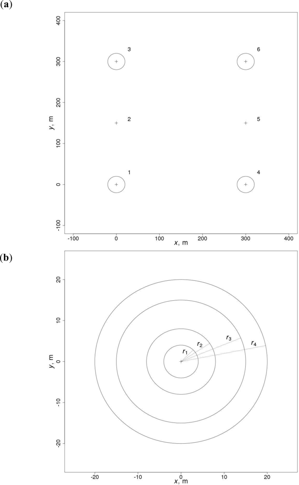
7] for local radiometric correction to assist with the multi-source forest inventory. In their study, the idea was to adjust the BRDF-affected intensities in digitized aerial photography to match the local intensities of the reference imagery, i.e., the Landsat 5 TM satellite data. Thus, the reference imagery needs to be independent of the BRDF. The local calibration was based on adjusting the mean values in a correction unit, for example, a moving circle with a radius of 40 m. Using a moving window, an adaptive correction based on the reference image digital numbers became possible; likewise, the parameters for the method were defined empirically.
In the case of Terai, approaches developed by both Tomppo et al.[8] and Tuominen and Pekkarinen [7] were combined to create a local correction model. The separate Landsat TM images were corrected by applying the correction function below (see Equation (1)) and by using MODIS image data as the underlying reference image. The objectives of the procedure presented here are as follows: (1) to match the mean and the variance of the data in both images by taking into account the differences in pixel sizes [8] and (2) to apply the correction locally [7] by using raster map algebra and a moving window approach to calculate the parameter values for the model.
The correction function (see Tomppo et al.[8]) applied for a pixel (x, y) was as follows:
f ^ i ( x , y ) = a i ( x , y ) × f i ( x , y ) + b i ( x , y )
where i (x, y) is the corrected data for the pixel (x, y) in band i, fi (x, y) is the uncorrected data in band i, and ai (x, y) and bi (x, y) are the parameters computed for the given pixel (x, y) in band i.
To calculate the parameters for the correction function (Equation (1)), averaging was first used to transform the Landsat image data to match the resolution of the MODIS reference image. The common pixel size of the images after averaging is later denoted by c. This study used the c-value of 500 m. The raster maps “avgLi”, “sdLi”, avgMj” and “sdMj”—which represent the mean and standard deviation values of the Landsat TM data and the MODIS data in the compatible spectral wavelength bands i and j, respectively—were thereafter calculated using a moving window approach with a window size of w × w pixels. Here, a 21 × 21 window neighborhood was utilized (w = 21), representing approximately a 10 km neighborhood for each pixel with the size of c. The raster maps with a pixel size of c were computed for both image datasets: target images (Landsat TM) and reference images (MODIS).
Parameters ai and bi in the correction function (Equation (1)) were calculated for each pixel (x, y) as follows:
a i ( x , y ) = sd Mj ( x , y ) / sd Li ( x , y ) and b i ( x , y ) = avg Mj ( x , y ) avg Li ( x , y ) × a i ( x , y )
where i denotes a Landsat TM band and j denotes a MODIS band that is compatible with i. This study used the MODIS bands 3, 4, 1, 2, 6 and 7 as compatible bands for the Landsat TM bands 1, 2, 3, 4, 5 and 7.
Finally, the correction model (Equation (1)) was applied in the original Landsat TM image data to produce locally corrected Landsat data in a MODIS reflectance value scale and at the original 30-m resolution. The coefficients ai and bi (see Equation (2)) of the correction function (Equation (1)) were local, being based on statistics from the neighborhood of each pixel (x, y). As a result, the Landsat TM pixel values were rescaled according to the local distribution parameters (mean and standard deviation) of the pixel values in the reference image bands.
In the correction approach of this study, each Landsat TM image had to first be processed separately, after which a mosaic of the corrected Landsat TM images was created. This mosaic was used as input for the forest/non-forest classification and the wall-to-wall map generation of a forest variable (stand volume, m3·ha−1).
The resolution (c) of the raster maps representing the mean and standard deviation and the size of the moving window (w) are user-defined parameters. Here, we used a resolution corresponding to that of the reference MODIS image, i.e., averaging was used only for Landsat images, as mentioned above. The size of the moving window (w) determines the flexibility of local correction. However, the window size (w) should be large enough to enable valid computations of the mean and standard deviation. In this case, it was not possible to conduct an exhaustive search for the resolution and neighborhood size (w), and therefore, we evaluated the result by checking the visual appearance of the resulting image mosaic. A good-quality reference image without any extreme pixel values is needed for a successful result.

3.2. Nearest Neighbors Techniques

A non-parametric, multi-source forest inventory method based on the k-nearest neighbor (k-NN) estimation (see Tomppo [4], Tomppo et al.[5]), an approach recently reviewed by McRoberts [25], was applied in the production of forest cover and volume maps in the Terai region. In this study, the population units (the target set of pixels) were the pixels in the satellite image. The satellite image bands were used as the ancillary variables (feature variables) with observations for all units of the population. The forest variables with observations only available for a sample (the reference set of pixels) were denoted as response variables. In practice, the reference set is built by querying the satellite image in the locations of sample plots, whereas the aim of the nearest neighbors approach is to impute the response variable values to the target set elements.
The classification was based on a pixel-by-pixel analysis, where the nearest neighbors for a target pixel among all the reference pixels (the pixels covering the center point of a sample plot) were determined using weighted Euclidean distance in spectral feature space (see Tokola [26]; for this in matrix form, see, e.g., McRoberts [25]):
d ij = h = 1 n b [ p h ( b ih b jh ) ] 2 ,
where nb is the number of bands, i is the target set element for which a prediction is sought and j is a reference set element, bih and bjh are spectral band values for the pixels i and j on band h, respectively, and ph is the empirical parameter for band h.
For the target pixel i, the k-nearest neighbors (i.e., a set of k reference pixels to which the Euclidean distance in spectral feature space from the target pixel i is smallest, K(i)={ j1(i),…, jk(i)}) were sought. In the case of categorical variables, the mode value of a response variable from among the k-nearest neighbors was the predicted class for a target pixel. In the case of continuous response variables, on the contrary, the weight wij of each neighbor jK(i) was determined to be inversely proportional to its distance to target pixel i:
w ij = d ij t / j K ( i ) d ij 1 ,
where t is a user-defined parameter (t ≥ 0).
In this study, a small positive number was given for zero distances and a value t = 2 was used in Equation (4). It follows that for target pixel i, j K ( i ) w ij = 1. A k-nearest neighbor prediction (ŷi) target pixel i was calculated as follows:
y ^ i = j K ( i ) w ij y j ,
where yj is the observed value of the response variable in reference pixel jK(i).
In forest cover mapping, the set of spectral features contained values of the image mosaic bands from 1 to 6, corresponding to the Landsat TM image bands from 1 to 5 and 7, and we used the Euclidean distance as the measure of distance (the band weight (ph) was set to 1 for all bands). The mode value of a response variable, i.e., the FAO land use class, among the k-nearest neighbors was the predicted class for the given target pixel. We selected pixels from the Landsat TM mosaic from Terai as the set of target pixels using the physiographic zone raster map as a mask in the GRASS GIS package. The reference set consisted of the pixels covered by the center points of the 1st phase plots, where the observed value (FAO land use class) was known based on the visual interpretation. In order to clarify forest classification, the plots belonging to the land use categories “Agricultural area with tree cover” or “Built-up area with tree cover” were dropped out from the reference set, whereas the category “Roads”, having a very small number of observations, was combined with the category “Built-up land without tree cover”.
The post-processing phase of the classification included three steps. First, we applied a spatial 3 × 3 mode filter to reduce the salt-and-pepper effect in the pixel-by-pixel classification. Second, we constructed a forest/non-forest raster map (denoted as a forest cover raster map later) by reclassifying non-forest categories into a single class. Third, we converted the resulting forest cover raster map into a vector format and excluded forest segments with an area of less than 0.5 ha.

3.3. Validation of Results

For the category variable, i.e., forest cover, the value for k was selected by examining the classification accuracy of the forest cover predictions obtained using different values of k. For classification accuracy, indicators based on the confusion matrices were used [27] and included: (1) producer’s accuracy (FPA, forest), (2) user’s accuracy (FUA, forest), (3) overall accuracy (OA) and (4) the Kappa statistic (KHAT); the KHAT was computed because the OA results are too optimistic if the proportion of a single class is high (see Hyvönen and Anttila [28]).
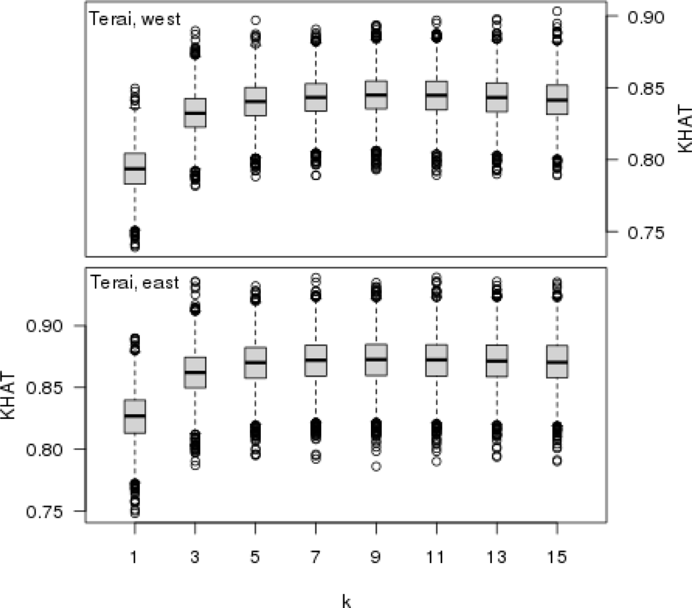
The Monte Carlo technique, including the random sampling of test samples, was applied when selecting k, i.e., the number of neighbors. For each k ∈ {1, 3, 5,...,15}, 5,000 test samples were randomly selected from the entire reference element set. Each sample contained 1,000 elements (1st phase sample plots of visual inspection), which were classified as test material, whereas all the remaining elements not included in the sample comprised the reference. The aforementioned classification accuracy indicators were calculated for each test sample. As a result, an empirical distribution of each test indicator with a varying value of k was produced. This approach was applied in the two parts of Terai separately. At the end, the forest cover delineations derived from the visual interpretation and the forest cover map were also checked by their classification accuracy using the field observed values for the field sample plots.
A leave-one-out analysis was conducted, and common cross-validation criteria, i.e., RMSE and bias, were calculated for the continuous variable, i.e., the total stand volume, in the reference set (e.g., Tokola [26]; Katila and Tomppo [29]). In this study, the RMSEs and biases were determined as follows:
RMSE = i = 1 n ( y i y ^ i ) 2 / n
bias = i = 1 n ( y i y ^ i ) / n ,
where yi is the observed value, ŷi the predicted value of the given characteristic, and n is the number of observations. The relative, i.e., percent, RMSEs (RMSE%) and biases (bias%) were calculated by dividing the absolute RMSEs and biases by the means of the respective values from the observations () and multiplying the resulting quotients by 100.
Cross-validation and feature selection were carried out using a genetic algorithm-based approach (e.g., Haapanen and Tuominen [30]) that has been compiled in with the “genalg” package of R software [31]. The value for k was simultaneously determined in the feature selection and weight search. Several runs were made in order to find the best combination of features and parameter value for k for the volume estimation. The parameter values of population size, number of iterations, elitism and mutation chance that we used for the algorithm were 500, 1,000, 40% and 0.05, respectively, and the goal was to minimize the sum of RMSE and bias obtained for the stand volume. The features that we tested for the model included band values (b1,…,b6) in the Landsat TM mosaic (referring to TM wavelength bands 1,..,5 and 7) together with the ratios of the band values and the value of the Normalized Difference Vegetation Index (NDVI).
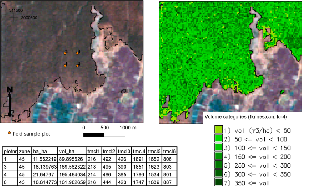
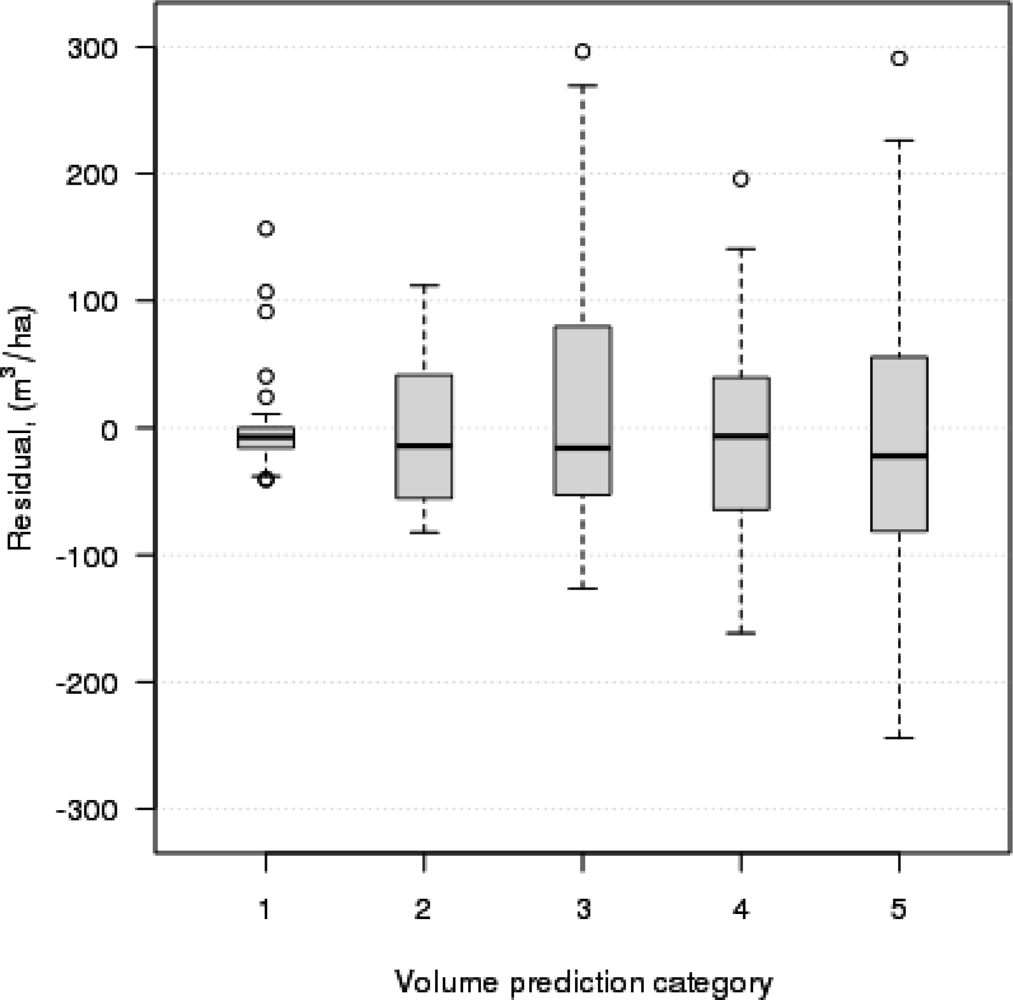
When creating thematic wall-to-wall maps for growing stock volume, we selected a set of target pixels using the forest cover map as a mask in the GRASS GIS package. The reference set consisted of the pixels covered by the center points of the field plots (Table 2). For composing the thematic map of volume, we classified the volume predictions for the pixels into classes of 50 m3·ha−1.

4. Results

4.1. Forest Cover Mapping

An example of an original Landsat TM image subset and the resulting image mosaic is shown in Figure 3(a–c). After inspecting the overall appearance of the image mosaic, it proved usable as input for the forest cover and volume mapping based on k-nearest neighbor techniques.
Kappa statistics (Figure 4) show that in forest cover mapping, using values of k greater than 5 does not improve the quality of the estimation result. For this reason, we set the value of k at 5 in forest cover mapping for both parts of Terai.
Other accuracy measures (Table 3) also support the decision made regarding the value of k and indicate that the accuracy is quite good in both parts of Terai; both the FUA and FPA are more than 85%, even in the case of k = 1.
Table 4 shows the confusion matrices of the forest cover delineations based on visual interpretation and the forest cover map against the one based on the observed values for the field sample plots (n = 217). The accuracy of the delineation of forest cover by visual interpretation is very good in both parts of Terai. In eastern Terai, the forest cover mapping based on the k-NN techniques appears to have the same accuracy level as the visual interpretation, but in western Terai, the user’s accuracy in the class “Non-forest” is slightly lower compared to other categories.
The confusion matrices between the forest cover map classification and the visual interpretation were also created (Table 5). In this examination, based on the set of field plot points only, the Kappa statistic shows a better agreement between the forest cover map and visual interpretation in eastern Terai compared to the western Terai, where the agreement can still be characterized as substantial [32].
A forest cover map for the entire Terai physiographic zone made by combining the results from the western and eastern parts of Terai is shown in Figure 5.

4.2. Thematic Map of a Forest Variable: Volume

The following features (spectral band values or ratios) were included in the model for the estimation of total stand volume: b1, b2, b4/b3 and b5/b3. The band weights (i.e., the parameters ph in Equation (3)) for the four variables in the weighted spectral Euclidean distance were as follows: 0.8537294, 0.9748646, 0.5139022 and 0.3661812, respectively. It was noted that several runs produced quite similar results. We used the values of 4 and 2 for parameters k and t, respectively, of which the former was obtained from the genetic algorithm. The RMSE and bias values obtained for the stand volume were 85.4 m3·ha−1 (62.0%) and −0.541 m3·ha−1 (slight overestimation effect), respectively. The boxplot [31] of residuals for the volume prediction categories of 50 m3·ha−1 show the presence of some extreme observations, whereas the median of residuals is close to zero in all categories (Figure 6).
Plotting the means for the ordered groups of observations against the means for the predictions for the same ordered groups (see McRoberts [33]) reveals that volume predictions suffer from averaging: the large volumes were underestimated and the small volumes were overestimated (Figure 7).

5. Discussion

In the case of the Terai region, it was not possible to apply the nearest neighbor’s techniques for each Landsat image separately, because the number of plots was inadequate. This meant that we needed to apply relative calibration for the Landsat images, despite the fact that there could be quite a long amount of time between the dates for the available good-quality images. For this purpose, we applied a pre-processing approach based on using a reference image covering the whole region. For aiming at a seamless result, the potential overlapping area of the neighboring target images (Landsat TM images in our case) needs to be utilized when the raster maps representing means and standard deviations are computed. By detecting pixels having extreme values (outlier pixels) in the images and excluding them from this stage, one can improve the result of this local approach. Depending on image materials, this method also allows one to apply a pixel size c different than the original pixel size in the reference image.
A robust regression approach would offer another empirically oriented approach for a relative calibration of image materials. Regressing the images for the selected reference image would make it possible to concurrently use neighboring images. In the case of the geographically wide Terai region, the robust regression approach was less applicable. However, in a multi-temporal case, a regression approach for relative radiometric calibration could possibly be applied when detecting changes in landscape, such as cuttings (e.g., [11,34,35]).
The agreement between the k-NN forest cover classification and the visual interpretation in Terai was strong, since the resulting value of KHAT was greater than 0.80 (see, e.g., Congalton [27] and Green [32]). The OA values were also high, which can at least be partly explained by the high proportion of the non-forest category. It is worth noting that we did not examine the effect of the post-processing phase (steps 1 to 3) when calculating the accuracy measures in the test samples for the selected value of k. Also, the classification accuracy of the forest cover map evaluated against field observed values showed that the agreement between these forest cover delineations is substantial (western Terai) or strong (eastern Terai).
The visual land use class interpretation process was conducted using Google Earth satellite imagery viewer [21], where the background imagery originated from the period between 2003 and 2010, together with additional RapidEye imagery from the year 2010. Due to shaded areas, haze and cloudiness, the visual interpretation work proved difficult in the case of some RapidEye images, and then, the interpretation was supported using satellite imagery available in Google Earth. Therefore, the time difference between these image materials could make a source of uncertainty to the interpretation process itself. In this study, an unwanted mixing of the forest class and the land use classes with some tree cover was tackled by dropping out the plots in classes “Agricultural area with tree cover” and “Built-up area with tree cover” from the reference set. For classification accuracy checking, a correct matching of the locations between field plots and the visual interpretation plots on the image is also crucial. Unfortunately, information to check this location accuracy was not available.
Besides RMSE and bias, robust measures for the quality of the k-NN-based estimation in terms of feature selection and cross-validation could be useful, especially in cases where the number of plots is small, which corresponds to this study (n = 217). For instance, in the k-nearest neighbor analysis for stand volume, the most extreme observations may also have affected the model parameter search, because the number of field plots was quite small. Therefore, the diagnostic approach suggested by McRoberts [33] for detecting outliers and influential observations could be very important for our work in the future.
The k-nearest neighbor technique, applied to the mapping of forest cover and stand volume in the Terai region of Nepal, is a straightforward procedure that has been efficiently utilized in Finland (see, e.g., Tomppo et al.[5] and Tomppo [4]). Moreover, this technique was also applied earlier by Tokola et al.[36] for classifying land use and for estimating timber volume and biomass in Nepal.
This was, however, one of the first forest mapping studies completely conducted using Open Source software tools and free packages. In this respect, it was natural that substantial efforts were needed to incorporate appropriate data processing techniques and suitable procedures and, especially, that the techniques and procedures were compatible for processing the remote sensing and inventory data.
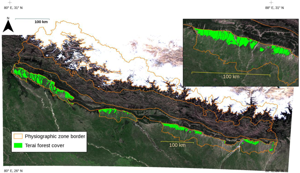
The forest cover map now available for Terai (Figure 5) is one source of information that can be utilized when estimating above-ground forest volumes and biomasses based on the LiDAR data as part of the ongoing survey conducted by the FRA Nepal project in the central parts of Terai. In the future, similar forest cover maps will also be needed for other physiographic zones beyond Terai, where the LiDAR-oriented estimations of forest attributes will be conducted. Later, experience will show if the forest cover maps prove useful in other fields of forestry. Potential applications in Nepalese conditions include inventory planning and monitoring practices. The forest cover and volume maps (Figure 8) estimated using the k-NN method and inventory data from the FRA Nepal project are already appropriate and valuable data for research purposes and for planning forthcoming forest inventories when testing optimal inventory designs (see [37]).
Spatially explicit biomass maps could also form a basis for the forthcoming greenhouse gas inventory, i.e., the REDD-related estimation of gross primary production and soil carbon change. The k-NN-based forest biomass mapping technique, which corresponds to that of stand volume mapping, has already been demonstrated by Tuominen et al.[38] in Finnish conditions. One shared feature between the approach by Tuominen et al.[38] and the one in this study has to do with the data-efficient, mixed-effects modeling-based generalization of sample tree characteristics. This study, however, used an NLME model for generalizing the sample tree heights (see Appendix), whereas the model utilized by Tuominen et al.[38] made use of an LME model provided by Eerikäinen [39].
Adapting the methods and techniques and applying the Open Source software tools presented here requires capacity building in Nepal: development work and education measures have already been launched by the ICI project, which is an inter-institutional development cooperation project between Nepalese, Vietnamese and Finnish governmental institutes and that was initiated with the support of the Ministry for Foreign Affairs (MFA) of Finland. The development activities of the project have been designed and implemented with a special focus on human capacity development within the governmental forest research organizations participating in the project. Special emphasis has therefore been given to hands-on training periods and workshops and to disseminating information on forest inventory-related techniques and procedures. Of these objectives, the latter covers the goal of the present study: to increase and share knowledge about the existing techniques and procedures and to make it easier to adapt them to the conditions in, for instance, Nepal.
Local expertise is always required for the most pivotal part of the forest inventory, that is to say, the work conducted in the field and, at the moment, by the FRA Nepal project in Nepal. Through scientific work and collaboration, however, it is possible to achieve more diverse and detailed results in terms of conventional statistics and advanced electronic maps of the forest attributes of interest. This study is also one example of how to improve the use of field inventory data and exploit them together with additional remote sensing data in order to satisfy the new reporting requirements set for large-scale forest inventories.

6. Conclusions

In this study, we introduced an approach for a MODIS-based relative calibration of Landsat TM images to enable the use of a mosaic of several Landsat TM images in a k-nearest neighbor (k-NN) estimation. The presented approach for relative calibration combined aspects presented earlier by Tuominen and Pekkarinen [7] and Tomppo et al.[8]. The method relies only on image data (see [7]) and is easy to implement. Optionally, the reference image could have been converted to a reflectance scale, but for the k-NN estimation method that was not necessary. A prerequisite for the success of the local correction approach for the relative calibration of images is that the target images and the good-quality reference image material need to be temporally and seasonally close to each other. However, more studies are needed on selecting the parameters for the approach when using image resolution scales other than the ones used in the Terai case, which utilized Landsat TM and MODIS.
The k-nearest neighbor technique was very applicable to the forest cover mapping in Terai using visual interpretation plots as a reference material. There was a strong agreement (KHAT > 0.80) between the forest cover delineations based on visual interpretation and field observations. The agreement between the forest cover delineation in the forest cover map and the one derived from the field observed values was substantial in Western Terai (KHAT 0.745) and strong in Eastern Terai (KHAT 0.825).
One feature related to the development of the multi-source technique and, especially, to its application to different geographical conditions in Nepal in the future has to do with using digital elevation models (DEMs). In the case of Terai, i.e., within the lowlands of Nepal, no radiometric corrections were conducted using DEMs (e.g., Tomppo et al.[5]; Tokola et al.[36]), neither was the DEM-based moving geographical vertical reference area used in the k-NN method (see Katila and Tomppo [29]). It is therefore recommended that the significance of DEM be tested in other physiographic vegetation zones north of Terai, where the topography is very mountainous compared to the southernmost region of Nepal.

Acknowledgments

This study was conducted at the Finnish Forest Research Institute’s (Metla) Regional Unit in Joensuu, Finland and the Department of Forest Research and Survey (DFRS) in Babarmahal, Kathmandu, Nepal. It was partly funded by the Ministry for Foreign Affairs of Finland through the inter-institutional development cooperation project entitled “Improving Research Capacity of Forest Resource Information Technology in Vietnam and Nepal” (contract number: HELM431-14, intervention code: 79811501). We are grateful to these institutions for their resources and funding. Support given by the Forest Resource Assessment of Nepal project is also gratefully acknowledged. Many thanks are also due to Juho Pitkänen for his help in developing the calculation procedures for this study.

References

  1. Acharya, K.P.; Dangi, R.B.; Tripathi, D.M.; Bushley, B.R.; Bhandary, R.R.; Bhattarai, B. (Eds.) Ready for REDD? Taking Stock of Experience, Opportunities and Challenges in Nepal; Nepal Foresters' Association: Kathmandu, Nepal, 2009.
  2. Pearson, T.; Walker, S.; Brown, S. Sourcebook for Land Use, Land-Use Change and Forestry Projects; Winrock International and the BioCarbon Fund of the World Bank: Washington, DC, USA, 2005; Available online: http://www.winrock.org/ecosystems/files/winrock-biocarbon_fund_sourcebook-compressed.pdf (accessed on 30 May 2012).
  3. GOFC-GOLD. A Sourcebook of Methods and Procedures for Monitoring and Reporting Anthropogenic Greenhouse Gas Emissions and Removals Caused by Deforestation, Gains and Losses of Carbon Stocks in Forests Remaining Forests, and Forestation, GOFC-GOLD Report version COP17-1; GOFC-GOLD Project Office, Natural Resources Canada: Edmonton, AB, Canada, 2011; Available online: http://www.gofcgold.wur.nl/redd/ (accessed on 20 September 2012).
  4. Tomppo, E. The Finnish Multi-Source National Forest Inventory—Small Area Estimation and Map Production. In Forest Inventory. Methodology and Applications; Managing Forest Ecosystems, Kangas, A., Maltamo, M., Eds.; Springer: Dordrecht, The Netherlands, 2006; Volume 10, pp. 195–224. [Google Scholar]
  5. Tomppo, E.; Haakana, M.; Katila, M.; Peräsaari, J. Multi-Source National Forest Inventory Methods and Applications; Managing Forest Ecosystems, Springer Science+Business Media: New York, NY, USA, 2008; Volume 18. [Google Scholar]
  6. Coppin, P.; Jonckheere, I.; Nackaerts, K.; Muys, B.; Lambin, E. Digital change detection methods in ecosystem monitoring: A review. Int. J. Remote Sens. 2004, 25, 1565–1596. [Google Scholar]
  7. Tuominen, S.; Pekkarinen, A. Local radiometric correction of digital aerial photographs for multi source forest inventory. Remote Sens. Environ. 2004, 89, 72–82. [Google Scholar]
  8. Tomppo, E.; Katila, M.; Mäkisara, K.; Peräsaari, J.; Malimbwi, R.; Chamuya, N.; Otieno, J.; Dalsgaard, S.; Leppänen, M. A Report to the Food and Agriculture Organization of the United Nations (FAO) in Support of Sampling Study for National Forestry Resources Monitoring and Assessment (NAFORMA) in Tanzania; FAO: Rome, Italy, 10 March 2010; Available online: http://www.mp-discussion.org/NAFORMA.pdf (accessed on 24 August 2012).
  9. Bodart, C.; Eva, H.; Beuchle, R.; Raši, R.; Simonetti, D.; Stibig, H.-J.; Brink, A.; Lindquist, E.; Achard, F. Pre-processing of a sample of multi-scene and multi-date Landsat imagery used to monitor forest cover changes over the tropics. ISPRS J. Photogramm. 2011, 66, 555–563. [Google Scholar]
  10. Tomppo, E.; Czaplewski, R.L.; Mäkisara, K. FRA 2000 The Role of Remote Sensing in Global Forest Assessment. A Remote Sensing Background Paper for Kotka IV Expert Consultation 01.07–05.07.2002, Kotka, Finland; Working Paper 61; Forest Resources Assessment Programme (FRA) of FAO: Rome, Italy, 2002; Available online: ftp://ftp.fao.org/docrep/fao/006/ad650e/ad650e00.pdf (accessed on 20 November 2012).
  11. Tokola, T.; Löfman, S.; Erkkilä, A. Calibration of multitemporal landsat data for forest cover change detection. Remote Sens. Environ. 1999, 68, 1–11. [Google Scholar]
  12. Open Foris Wiki. Available online: http://km.fao.org/OFwiki/index.php/Main_Page (accessed on 26 June 2012).
  13. Lillesø, J.-P.B.; Shrestha, T.B.; Dhakal, L.P.; Nayaju, R.P.; Shrestha, R. The Map of Potential Vegetation of Nepal: A Forestry/Agroecological/Biodiversity Classification System; Development and Environment Series 2–2005 and CFC-TIS Document Series No. 110; Forest & Landscape: Aalborg, Denmark, 2005. [Google Scholar]
  14. MODIS Products Table. Available online: https://lpdaac.usgs.gov/products/modis_products_table (accessed on 18 June 2012).
  15. MODIS Reprojection Tool. Available online: https://lpdaac.usgs.gov/tools/modis_reprojection_tool (accessed on 26 June 2012).
  16. GDAL: Geospatial Data Abstraction Library. Available online: http://www.gdal.org/index.html (accessed on 18 June 2012).
  17. Quantum GIS. Available online: http://www.qgis.org/ (accessed on 18 June 2012).
  18. Neteler, M.; Mitasova, H. Open Source GIS: A GRASS GIS Approach, 3rd ed.; Springer Science+Business Media: New York, NY, USA, 2008. [Google Scholar]
  19. Kleinn, C. Forest Resources Inventories in Nepal: Status Quo, Needs, Recommendations; FRIS Project Paper No. 1; Forest Resource Information System Project (FRISP), HMGN/FINNIDA, Finnish Forest and Park Service: Kathmandu, Nepal, 1994. [Google Scholar]
  20. Forest Resource Assessment of Nepal. Draft Field Manual 2010; Version of October 16, 2010; Forest Resource Assessment of Nepal Project: Kathmandu, Nepal, 2010. [Google Scholar]
  21. Google Earth. Available online: http://www.google.com/earth/index.html (accessed on 26 June 2012).
  22. van Laar, A.; Akça, A. Forest Mensuration; Cuvillier Verlag: Göttingen, Germany, 1997. [Google Scholar]
  23. Sharma, E.R.; Pukkala, T. Volume Equations and Biomass Prediction of Forest Trees of Nepal; Publication 47; Forest Survey and Statistics Division, Ministry of Forests and Soil Conservation: Kathmandu, Nepal, 1990. [Google Scholar]
  24. Pinheiro, J.C.; Bates, D.M. Mixed-Effects Models in S and S-PLUS; Corrected third printing; Springer-Verlag: New York, NY, USA, 2002. [Google Scholar]
  25. McRoberts, R.E. Estimating forest attribute parameters for small areas using nearest neighbors techniques. Forest Ecol. Manag. 2012, 272, 3–12. [Google Scholar]
  26. Tokola, T. The Influence of Field Sample Data Location on Growing Stock Volume Estimation in Landsat TM-based Forest Inventory in Eastern Finland. Remote Sens. Environ. 2000, 74, 422–431. [Google Scholar]
  27. Congalton, R.G.; Green, K. Assessing the Accuracy of Remotely Sensed Data: Principles and Practices, 2nd ed.; CRC Press: Boca Raton, FL, USA, 2009. [Google Scholar]
  28. Hyvönen, P.; Anttila, P. Change detection in boreal forests using bi-temporal aerial photographs. Silva Fenn. 2006, 40, 303–314. [Google Scholar]
  29. Katila, M.; Tomppo, E. Selecting estimation parameters for the Finnish multisource National Forest Inventory. Remote Sens. Environ. 2001, 76, 16–32. [Google Scholar]
  30. Haapanen, R.; Tuominen, S. Data combination and feature selection for multi-source forest inventory. Photogramm. Eng. Remote Sensing 2008, 74, 869–880. [Google Scholar]
  31. R Development Core Team. R: A Language and Environment for Statistical Computing; R Foundation for Statistical Computing: Vienna, Austria, 2011; Available online: http://www.R-project.org/ (accessed on 2 December 2011).
  32. Landis, J.R.; Koch, G.G. The measurement of observer agreement for categorical data. Biometrics 1977, 33, 159–174. [Google Scholar]
  33. McRoberts, R.E. Diagnostic tools for nearest neighbors techniques when used with satellite imagery. Remote Sens. Environ. 2009, 113, 489–499. [Google Scholar]
  34. Varjo, J. Change detection and controlling forest information using multi-temporal Landsat TM imagery. Acta For. Fenn. 1997, 258, 1–64. [Google Scholar]
  35. Olsson, H. Regression functions for multitemporal relative calibration of Thematic Mapper data over boreal forest. Remote Sens. Environ. 1993, 46, 89–102. [Google Scholar]
  36. Tokola, T.; Sarkeala, J.; van der Linden, M. Use of topographic correction in Landsat TM-based forest interpretation in Nepal. Int. J. Remote Sens. 2001, 22, 551–563. [Google Scholar]
  37. Katila, M.; Tomppo, E. Sampling Simulation on Multi-Source Output Forest Maps—An Application for Small Areas. Proceedings of 7th International Symposium on Spatial Accuracy Assessment in Natural Resources and Environmental Sciences, Lisbon, Portugal, 5–7 July 2006; pp. 614–623.
  38. Tuominen, S.; Eerikäinen, K.; Schibalski, A.; Haakana, M.; Lehtonen, A. Mapping biomass variables with a multi-source forest inventory technique. Silva Fenn. 2010, 44, 109–119. [Google Scholar]
  39. Eerikäinen, K. A multivariate linear mixed-effects model for the generalization of sample tree heights and crown ratios in the Finnish National Forest Inventory. Forest Sci. 2009, 55, 480–493. [Google Scholar]
Figure 1. Map of Nepal with borders of the physiographic zones. The study area, i.e., Terai, is denoted by the grey-fill color.
Remotesensing 04 03920f1
Figure 2. Layout of the inventory cluster (a) and Concentric Circular Sample Plot (CCSP) (b) used in the FRA Nepal project. In the case of Terai, one cluster comprises four CCSPs (1, 3, 4 and 6) in a square with 300 m sides, i.e., plots number 2 and 5 of the basic cluster, which are used in the visual interpretation (first stage sample) and are excluded from the field inventory (second stage sample). In (b), the symbols r1,..., r4 are for the radii of the four circular plots (4, 8, 15 and 20 m, respectively) within the CCSP.
Remotesensing 04 03920f2
Figure 3. (a) Subsets of two original Landsat TM images from a region in Eastern Terai (Feb-4- 2010 for the image on the left and Jan-28- 2010 for the image on the right), a composite of TM bands 3, 2 and 1 (rgb). (b) A subset of the corrected Landsat TM image mosaic, a composite of TM bands 3, 2 and 1 (rgb). (c) A subset of the corrected Landsat TM image mosaic, a composite of TM bands 5, 3 and 2 (rgb). (Coordinate reference system: WGS 84/ UTM zone 45N).
Remotesensing 04 03920f3aRemotesensing 04 03920f3b
Figure 4. Distributions of KHAT statistic values at different k values in the western (upper figure) and eastern (lower figure) parts of Terai. In the boxplot, the grey region is the area between the 1st and 3rd quartiles (including 50% of the observations), the thick line is the median and the outer lines extend to the data point, which is no more than 1.5 times the area between the 1st and 3rd quartiles away from the box. The most extreme individual observations are also plotted [31].
Remotesensing 04 03920f4
Figure 5. A forest cover map (forest: bright green color) for the Terai physiograhic zone produced by the k-NN technique and overlaid on a composite of MODIS image bands 1, 4 and 3 (rgb).
Remotesensing 04 03920f5
Figure 6. Volume residuals in volume prediction categories of 50 m3·ha−1.
Remotesensing 04 03920f6
Figure 7. Mean observation versus mean prediction for volume (m3·ha−1). The observations have been sorted and grouped into groups of 20 observations at the minimum based on the observed volume (m3·ha−1).
Remotesensing 04 03920f7
Figure 8. At left: forest cover map (vector boundaries) and a field sample plot cluster, (plotnr = sample plot number; zone = UTM zone number; ba_ha = basal area, m2·ha−1; vol_ha = volume, m3·ha−1; tmcl1–tmcl6 = pixel values in the Landsat TM mosaic bands 1–6). At right: A thematic map of the volume. An example from eastern Terai (background: a composite of Landsat TM mosaic bands 5, 3 and 2 (rgb)). (Coordinate reference system: WGS 84/UTM zone 45N).
Remotesensing 04 03920f8
Table 1. Information about the Landsat TM satellite imagery used in this study. Path and row information is given in the WRS-2 system.
AreaDatePathRow
Western Terai2011-03-0714440
2010-02-2514341
2010-02-1814241

Eastern Terai2010-02-1114141
2010-02-0414041
2010-02-0414042
2010-01-2813942
Table 2. Descriptive statistics for the CCSP data, (n = 217): Dg is the basal area weighted mean diameter at breast height (cm), Hg is the basal area weighted mean height (m), N is the number of living trees (ha−1), G is the stand basal area of living trees (m2·ha−1) and V is the stand volume of living trees (m3·ha−1).
VariableMinimumMedianMeanStandard DeviationMaximum
Dg0.0035.6436.9525.70145.11
Hg0.0017.4416.139.2340.00
N0288.5473.6546.32735.5
G0.0016.0915.0010.4543.31
V0.00130.94137.53112.66499.59
Table 3. Statistics (mean and standard deviation (sd)) by the four indicators of classification accuracy (ICA): (1) the user’s accuracy of forest class (FUA), (2) the producer’s accuracy of forest class (FPA), (3) overall accuracy (OA) and (4) Kappa statistic (KHAT) based on the test samples for each value of k.
AreaICAValue of k
13579111315
Western TeraiFUAmean0.8660.8860.8890.8910.8910.8910.8890.888
sd0.0170.0160.0150.0150.0160.0160.0160.016
FPAmean0.8700.9010.9080.9100.9110.9120.9120.911
sd0.0170.0150.0140.0130.0130.0130.0130.013
OAmean0.9050.9230.9260.9280.9280.9280.9270.927
sd0.0070.0070.0070.0070.0070.0070.0070.007
KHATmean0.7930.8320.8400.8430.8450.8450.8430.841
sd0.0160.0150.0140.0140.0140.0150.0150.015

Eastern TeraiFUAmean0.8570.8970.9050.9080.9080.9080.9070.906
sd0.0260.0240.0230.0230.0230.0230.0230.024
FPAmean0.8520.8710.8760.8770.8780.8770.8770.877
sd0.0260.0240.0240.0240.0240.0240.0240.024
OAmean0.9530.9630.9660.9660.9660.9660.9660.966
sd0.0050.0050.0050.0050.0050.0050.0050.005
KHATmean0.8260.8620.8700.8720.8720.8720.8710.870
sd0.0200.0190.0190.0190.0190.0190.0190.019
Table 4. Confusion matrices between the forest cover delineations derived from the visual interpretation (Visual), the forest cover map and the field observations (Obs.). (UA = User’s accuracy, PA = producer’s accuracy, OA = overall accuracy, KHAT = Kappa statistic).
AreaObs.Visual Interpretation
Forest Cover Map
ForestNon-ForestTotalPA, %ForestNon-ForestTotalPA, %
Western TeraiForest103510895.4100810892.6
Non-Forest4283287.55273284.4


Total1073314010535140
UA, %96.384.895.277.1
OA, %93.690.7
KHAT0.8200.745

Eastern TeraiForest6126396.86126396.8
Non-Forest2121485.72121485.7


Total631477631477
UA, %96.885.796.885.7
OA, %94.894.8
KHAT0.8250.825
Table 5. Confusion matrices between the forest cover map and the forest cover delineation derived from the visual interpretation (Visual). (UA = User’s accuracy, PA = producer’s accuracy, OA = overall accuracy, KHAT = Kappa statistic).
AreaVisualForest Cover Map
ForestNon-ForestTotalPA, %
Western TeraiForest971010790.7
Non-Forest8253375.8

Total10535140
UA, %92.471.4
OA, %87.1
KHAT0.650

Eastern TeraiForest6126396.8
Non-Forest2121485.7

Total631477
UA, %96.885.7
OA, %94.8
KHAT0.825

Appendix: Height Prediction Model

A1.1. Modeling Data

The sample tree data available for modeling the relationship between height and diameter comprised 1,048 trees measured on 182 field sample plots within 56 clusters. The total number of species was 93, including an “unknown” group. Descriptive statistics for the tree-level and sample plot-level characteristics used in the modeling are given in Table A1.
Table A1. Descriptive statistics for the tree-level and plot-level characteristics of the height modeling data: h is the total tree height (m); zdominated and zdominant are dummy variables for the dominated and dominant tree, respectively; G is the stand basal area at the plot-level (m2·ha−1); zKS/SK, zSB and zTMH are plot-level dummy variables for the forest types of Khair Sissoo Forest, Shrub, and Terai Mixed Hardwood Forest, respectively; zSG1zSG4 are tree-level dummy variables for species groups 1–4, respectively; and d is the tree diameter at breast height (cm).
VariableMinimumMedianMeanStandard DeviationMaximum
h2.0015.9516.887.67141.10
zdominated000.050.2251
zdominant010.820.3851
G0.5119.9320.587.90843.31
zKS/SK000.020.1261
zSB000.000.0531
zTMH010.600.4911
zSG1000.430.4951
zSG2000.130.3331
zSG3000.250.4321
zSG4000.200.4001
d5.027.432.3021.516187.9

A1.2. Model Specification

The sample tree heights were generalised to cover the tally trees using a mixed modeling technique proposed, for instance, by Lappi [A1] and Eerikäinen [39]. Instead of linear model forms, which were used by Lappi [A1] and Eerikäinen [39], this study utilized a nonlinear, mixed-effects modeling (NLME) procedure (see, e.g., Pinheiro & Bates [24]). Eerikäinen [39] estimated species-specific effects using dummy variables, which were treated not only as fixed but also as random variables, and determined the species effects for Scots pine, Norway spruce and a group of broadleaved trees. In Terai case, however, an automated pooling procedure for grouping species into crown layer classes was constructed. In the pooling procedure, a candidate model localised by clusters and sample plots, respectively, was used to determine whether the majority of the species-wise observations belonged to the group of heights that were equal to or greater than the model prediction or to the group of observations that were less than the model prediction. After separating the height data by species into two crown layers, the same modeling and sorting procedure was conducted for both sets of data, resulting in the fact that the observations were finally aggregated into four groups of consecutive crown layers by species.
The random components of the models were related to the intercept term and the coefficient of the tree size variable, i.e., the diameter at breast height, respectively, of which the latter term was also associated with the components for random species effects (see also Eerikäinen [39]). An NLME model for a tree height (hijk, m) having a random intercept and slope terms with respect to the cluster (u(1)) and sample plot (u(2)) effects as well as the tree species effects for the four crown layer groups can now be described under conditions of normality (N) as follows:
h ijk = 1.3 + ( ( β 1 + u 1 , i ( 1 ) + u 1 , i j ( 2 ) ) + β 2 × z dominated ijk + β 3 × z dominant ijk + β 4 × ln ( G ij + 1 ) + β 5 × z KS / SK ij + β 6 × z SB ij + β 7 × z TMH ij ) × exp ( ( ( β 8 + u 8 , i ( 1 ) + u 8 , i j ( 2 ) ) + ( β 8.1 + u 8.1 , i ( 1 ) + u 8.1 , i j ( 2 ) ) × z SG 1 ijk + ( β 8.3 + u 8.3 , i ( 1 ) + u 8.3 , i j ( 2 ) ) × z SG 3 ijk + ( β 8.4 + u 8.4 , i ( 1 ) + u 8.4 , ij ( 2 ) ) × z SG 4 ijk ) × ( d ijk + λ d ) β 9 ) + e ijk , for which [ u 1 , i ( 1 ) u 8.4 , i ( 1 ) ] N ( 0 , Ω u ( 1 ) ) : Ω u ( 1 ) = [ σ u 1 ( 1 ) 2 σ u 1 ( 1 ) u 8.4 ( 1 ) σ u 8.4 ( 1 ) u 1 ( 1 ) σ u 8.4 ( 1 ) 2 ] [ u 1 , i j ( 2 ) u 8.4 , i j ( 2 ) ] N ( 0 , Ω u ( 2 ) ) : Ω u ( 2 ) = [ σ u 1 ( 2 ) 2 σ u 1 ( 2 ) u 8.4 ( 2 ) σ u 8.4 ( 2 ) u 1 ( 2 ) σ u 8.4 ( 2 ) 2 ] , e ijk N ( 0 , σ e 2 ) ,
where β1, β2,..., β8.4, β9 and λd are fixed model parameters; i, j and k refer to the cluster, plot and tree, respectively; zdominatedijk and zdominantijk are dummy variables for the dominated and dominant tree, respectively; Gij is the stand basal area at the plot j of cluster i (m2·ha−1); zKS/SKij, zSBij and zTMHij are dummy variables for three forest types, a Khair Sissoo Forest, a Shrub Forest and a Terai Mixed Hardwood Forest, respectively; dijk is the diameter at breast height (cm); zSG1ijk,zSG3ijk and zSG4ijk are dummy variables for the species groups 1, 3 and 4, respectively (note: when zSG1ijk, zSG3ijk and zSG4ijk are set to zero, the predictions are obtained for species group 2 (SG2)); and eijk is the random error term of the model.
The parameter λd in Equation (A1) was added to the independent variable “dijk” in order to decrease the residual variation among small-sized trees. The selection of fixed values for λd and for the form parameter β9 was based on the analysis of residuals as well as the Akaike Information Criterion (AIC) values (see [24]) and Root Mean Square Errors (RMSEs, see Equation (6)) obtained using different values for the two parameters (see also Eerikäinen et al. [A2]). A combination of values of 10 and 0.65 for the respective parameters λd and β9 was found to provide the best model fit in the PSP data from Terai.
The variance functions are useful for accounting for the within-group heterogeneous variances when, for instance, the error variance increases as the tree size increases (see [24,A3]). Thus, they are also useful for improving the convergence properties of the algorithms used for the estimation of parameters of LME and NLME models. The variance functions include the variance model’s power type (see [24,A4,A5]):
var ( e ijk ) = σ e 2 × | v ijk | ( 2 × δ m )
which corresponds to the variance function
g ( v ijk , δ m ) = | v ijk | δ m ,
where vijk is a weighting variable, e.g., the diameter at breast height or its transformation, and δm is an unrestricted, group-dependent parameter that needs to be estimated and which assumes values according to the stratification variable m respective to the four species effect groups (i.e., SG1–SG4). The appropriate weighting variable (vijk) of the variance function was found to be (dijk+5).

A1.3. Parameter Estimation and Model Validation

The parameters of the NLME model for tree height in Terai were estimated using the R package, a free software environment for statistical computing and graphics [31]. Modeling was technically implemented using the “nlme()” function from the library entitled “nlme”, which provides Maximum Likelihood (ML) estimates for parameters.
In the case of modeling data, localised height/diameter curves are directly obtained by extracting the estimates of the random effects for the model using a generic function “ranef()” of the library “nlme()”. However, when the NLME models, such as Equation (A1), are applied outside their modeling data, the localisation can be based on the predictor proposed by Vonesh and Chinchilli [A6], a procedure also applied and demonstrated by Crecente-Campo et al. [A7] in the derivation of predicted values of the random effects.
The criteria for selecting the independent variables for the height generalization model were the significance and logical signs of the estimated coefficients. The significance test for fixed model parameters (t-test) was used to test whether or not the true value of a parameter was zero: all the fixed parameters were treated as significant at the conservative preset level of 0.05. In addition, scatter plots in which the residuals were shown as functions of the height estimates and values of the independent variables were inspected. The candidate nonlinear mixed-effects (NLME) models were validated using the modeling data with the ML parameter estimates, employing as criteria the AIC values. Additionally, estimates of the RMSE and bias (see Equations (6) and (7)) were determined for the candidate models when quantifying the residual variation and assessing the impacts of transformations and alternative parameterisations on the prediction accuracy of the models.
The automated pooling procedure for grouping species into four crown layer classes resulted in the numbers of species being 19, 16, 24 and 34 with respect to the crown layer classes 1, 2, 3 and 4. The total number of individual height sample trees (n = 1048) for the crown layer classes 1–4 were 446, 133, 259 and 210, respectively. The estimates obtained for the fixed parameters of the NLME height model (Equation (A1)) are given in Table A2. The estimates for the fixed parameters of the NLME model clearly show that the parameters are significant and that their signs are logical (see Table A2).
When inspecting the estimates given in Table A3 for random parameters for the cluster and plot effects and the associated species effects, respectively, it is possible to conclude that they were substantially correlated, which is in line with earlier findings by Eerikäinen [39].
Table A2. Parameter estimates for the fixed independent variables of the NLME model for tree height (Equation (A1)).
ParameterEstimateStandard Errort-valuep-value
β120.100563.476975.78<0.001
β2−10.934931.83761−5.95<0.001
β35.392721.077085.01<0.001
β48.319910.957198.69<0.001
β5−8.469842.99058−2.830.005
β614.155765.563162.540.011
β7−3.137940.99325−3.160.002
β811.797720.3759031.39<0.001
β8.1−1.023560.21786−4.70<0.001
β8.31.290690.241345.35<0.001
β8.42.280250.251129.08<0.001
Table A3. Estimated Variances (diagonal), covariances (lower triangle) and correlations (upper triangle) for the random parameters of Equation (A1) at the cluster, plot and tree levels, respectively, and estimates for the power parameters of the variance function respective to the four species groups, i.e., SG1–SG4 (Equation (A3)).
Cluster Level
u 1 ( 1 ) u 8 ( 1 ) u 8.1 ( 1 ) u 8.3 ( 1 ) u 8.4 ( 1 )

u 1 ( 1 )50.2490450.8360.604−0.1750.529
u 8 ( 1 )7.7909491.7283850.076−0.6630.548
u 8.1 ( 1 )0.8564610.0199870.0400140.5890.056
u 8.3 ( 1 )−0.770911−0.5416710.0732190.386193−0.037
u 8.4 ( 1 )2.0149780.3871250.006019−0.0123550.288736

Plot Level
u 1 ( 2 ) u 8 ( 2 ) u 8.1 ( 2 ) u 8.3 ( 2 ) u 8.4 ( 2 )

u 1 ( 2 )27.8941140.4060.9530.6380.762
u 8 ( 2 )0.4342410.0410110.6590.946−0.268
u 8.1 ( 2 )4.8703310.1291350.9363080.8390.536
u 8.3 ( 2 )0.9807050.0557570.2362830.0847080.012
u 8.4 ( 2 )1.141066−0.0153880.1470530.0009900.080389

Tree Level
e

e0.194484

Estimates for the Power Parameters
δSG1δSG2δSG3δSG4

0.5459920.4924960.4996640.503056
The bias and RMSE values obtained for the localised model in the modeling data (n = 1,048) were 0.05 m (0.3%) and 2.74 m (16.3%), respectively. When calculated by the crown layer classes, the RMSE values were 3.20 m (15.5%), 2.24 m (14.0%), 2.47 m (16.3%) and 2.26 m (19.8%), respectively, whereas the bias values were 0.26 m (1.2%), −0.05 m (−0.3%), −0.08 m (−0.5%) and −0.16 m (−1.4%), respectively. It is possible to conclude that the magnitude of variation in the RMSE and bias values obtained from the crown layer classes for height predictions remains quite consistent.

References

  1. Lappi, J. Calibration of height and volume equations with random parameters. Forest Sci. 1991, 37, 781–801. [Google Scholar]
  2. Eerikäinen, K.; Mabvurira, D.; Nshubemuki, L.; Saramäki, J. A calibrateable site index model for Pinus kesiya plantations in southeastern Africa. Can. J. Forest Res. 2002, 32, 1916–1928. [Google Scholar]
  3. Lappi, J. A longitudinal analysis of height/diameter curves. Forest Sci. 1997, 43, 555–570. [Google Scholar]
  4. Hall, D.B.; Clutter, M. Multivariate multilevel nonlinear mixed effects models for timber yield predictions. Biometrics 2004, 60, 16–24. [Google Scholar]
  5. Wutzler, T.; Wirth, C.; Schumacher, J. Generic biomass functions for Common beech (Fagus sylvatica) in Central Europe: predictions and components of uncertainty. Can. J. Forest Res. 2008, 38, 1661–1675. [Google Scholar]
  6. Vonesh, E.F.; Chinchilli, V.G. Linear and Nonlinear Models for the Analysis of Repeated Measurements; Chapman and Hall: London, UK, 1997. [Google Scholar]
  7. Crecente-Campo, F.; Tomé, M.; Soares, P.; Diéguez-Aranda, U. A generalized nonlinear mixed-effects height–diameter model for Eucalyptus globulus L. in northwestern Spain. Forest Ecol. Manag. 2010, 259, 943–952. [Google Scholar]

