Article

Calibration of a Species-Specific Spectral Vegetation Index for Leaf Area Index (LAI) Monitoring: Example with MODIS Reflectance Time-Series on Eucalyptus Plantations

1
Eco&Sols, 2 Place Viala - bât 12, 34060 Montpellier cedex 01, France
2
SupAgro, UMR Eco&Sols, 2 Place Viala - bât 12, 34060 Montpellier cedex 01, France
3
Departamento de Ciências Atmosféricas, IAG, Universidade de São Paulo, Cidade Universitária-SP, 05508-090, Brazil
4
Department of Forestry and Environmental Sciences, North Carolina State University, Raleigh, NC 27695, USA
5
Remote Sensing Department, National Institute for Space Research (INPE), São José dos Campos-SP, 12227-010, Brazil
*
Author to whom correspondence should be addressed.
Remote Sens. 2012, 4(12), 3766-3780; https://doi.org/10.3390/rs4123766
Submission received: 10 October 2012 / Revised: 20 November 2012 / Accepted: 21 November 2012 / Published: 27 November 2012

Abstract

:
The leaf area index (LAI) is a key characteristic of forest ecosystems. Estimations of LAI from satellite images generally rely on spectral vegetation indices (SVIs) or radiative transfer model (RTM) inversions. We have developed a new and precise method suitable for practical application, consisting of building a species-specific SVI that is best-suited to both sensor and vegetation characteristics. Such an SVI requires calibration on a large number of representative vegetation conditions. We developed a two-step approach: (1) estimation of LAI on a subset of satellite data through RTM inversion; and (2) the calibration of a vegetation index on these estimated LAI. We applied this methodology to Eucalyptus plantations which have highly variable LAI in time and space. Previous results showed that an RTM inversion of Moderate Resolution Imaging Spectroradiometer (MODIS) near-infrared and red reflectance allowed good retrieval performance (R2 = 0.80, RMSE = 0.41), but was computationally difficult. Here, the RTM results were used to calibrate a dedicated vegetation index (called “EucVI”) which gave similar LAI retrieval results but in a simpler way. The R2 of the regression between measured and EucVI-simulated LAI values on a validation dataset was 0.68, and the RMSE was 0.49. The additional use of stand age and day of year in the SVI equation slightly increased the performance of the index (R2 = 0.77 and RMSE = 0.41). This simple index opens the way to an easily applicable retrieval of Eucalyptus LAI from MODIS data, which could be used in an operational way.

1. Introduction

The Leaf Area Index (LAI), defined as the surface of leaves per square meter of soil (m2·m−2), is a key characteristic of forest ecosystems. It is involved in many ecological processes such as light interception, photosynthesis and transpiration. Its quantification on different time and space scales is therefore crucial for a variety of subjects involving carbon, water and/or surface energy fluxes. Field estimations of LAI are costly and tedious, especially for forest ecosystems. The use of remotely-sensed images taken from sensors onboard aircraft or satellites offers the opportunity to estimate this variable on different spatial scales and dates.
The reflectance of a canopy scene results from the interaction of incident light with the different objects constituting the scene, and varies as a function of their arrangement and properties. In the case of forests, light interacts in a complex way with leaves, branches, trunks, soil, etc., which each have specific properties and are organized together in a given three-dimensional arrangement. The geometry of measurement and illumination, and atmospheric effects bring additional complexity to the reflectance signal that a sensor measures. The corollary is that the reflectance of a forest contains information about some of the characteristics of the forest. In particular, the reflectances in the near-infrared (NIR) region and in the red part of the visible wavelengths are sensitive to LAI, e.g., [1].
Different approaches exist to retrieve the LAI from measured reflectance. Compared to more complex methods like radiative transfer model (RTM) inversion, the use of empirical spectral vegetation indices (SVIs) remains an attractive method due to its simplicity of application, its robustness, and the fact that only few bands present in multispectral images taken from earth observation satellites are usually needed. The RVI (the ratio between the reflectances of NIR and red bands, also named SR) [2] and the widely used NDVI index (NDVI = (NIR – Red)/(NIR + Red)) [1] are very simple SVIs, often shown to correlate with LAI but to saturate for high LAI values, e.g., [3]. More complex SVIs were then developed, for example by taking into account soil reflectance, like the “soil adjusted vegetation index” (SAVI) family of indices [4]. SVIs using other spectral bands or other sources of information have been proposed to correlate with LAI, like the enhanced vegetation index (EVI) which uses the blue band [5,6] or the Reduced Simple Ratio (RSR) which uses the short-wave infrared (SWIR) band [7]. To generalize the definition and use of SVIs for LAI assessment, we can state that SVI methodologies link the reflectance to the LAI with an empirical function consisting in:
  • The use of the reflectance of some specific spectral bands (e.g., NIR, red wavebands),
  • The combination of these reflectance bands in a given mathematical formula, with the possibility of weighting these reflectances, which gives the SVI value,
  • The use of a linear or nonlinear model between SVI and LAI to retrieve LAI from SVI. This relationship may or may not use additional external information.
However, it has often been demonstrated that: (1) some SVIs may perform better than others depending on vegetation types, e.g., [8]; (2) some SVIs have to be adjusted locally to take into account differences in soil reflectance, e.g., [4]; (3) the relationship between SVI and LAI is often imprecise, or varies with space, time, and/or plant species, e.g., [9,10]; (4) the geometry of acquisition, atmospheric effects and sensor specificities may influence the vegetation indices, e.g., [11,12]. As a result, SVIs need to be calibrated locally.
In this study, we developed an approach that consists in building a species-specific SVI, i.e., an index constructed by calibrating all of the three points (a), (b) and (c) presented above—and not only (c) as is generally done—for a given vegetation species. A general SVI designed to correlate with LAI may also be influenced by other biophysical or biochemical properties of the vegetation [13]. In contrast, a species-specific SVI would minimize these effects while maximizing the correlation with LAI for a given species, by choosing a more adequate combination of bands and/or relationship between SVI and LAI. The main issue of producing a reliable species-specific SVI is that a very large number of field measurements are necessary to calibrate (a), (b) and (c) properly, covering as many configurations as possible (both of canopy characteristics and of image acquisition characteristics) and including repetitions. We aimed to alleviate this constraint by capitalizing on previous results obtained with the inversion of the PROSAIL forest radiative transfer model [14].
RTM simulate forest reflectance from canopy characteristics (LAI, leaf angle distribution, leaf chlorophyll content, soil reflectance, etc.), or alternatively can be inverted to estimate canopy characteristics from measured reflectance values and corresponding image acquisition geometry [15]. Eucalyptus canopy LAI was inverted from time series of MODIS reflectance data, with the other canopy characteristics (RTM biophysical input parameters) estimated as a function of stand age [14]. This method allowed good LAI retrieval results, and showed better efficiency than a method based on a soil adjusted SVI, the GESAVI [16]. It was, however, computationally intensive and difficult to apply operationally by non-specialists. In this study, we present a method that combines the accuracy of the RTM inversion method with the simplicity of application of a species-specific SVI: it relies on the calibration of the SVI using a “semi-empirical” dataset, derived from MODIS-measured reflectance and RTM-inverted LAI. The calibration dataset is thus (indirectly) based on a manageable number of field measurements (those required to validate the LAI estimations of RTM inversion), and nevertheless contains a very large number of LAI-reflectance combinations, corresponding to realistic and representative canopy and viewing/illumination conditions. In short, this methodology estimates an “inverted LAI” from the measured reflectance, i.e., mimics RTM inversion through a simple vegetation index.
This paper describes the calibration of a species-specific SVI using a semi-empirical dataset obtained from RTM inversion (note that the RTM inversion procedure is not presented in detail as it is fully described in [14]). The SVI presented here is called “EucVI”, and was designed for the estimation of stand LAI on fast-growing Brazilian Eucalyptus plantations, using MODIS time-series data. We also show how additional information derived from the reflectance time-series (i.e., in this case, stand age) can be incorporated in the SVI to improve its performance for LAI estimation.

2. Material and Methods

2.1. Study Site and LAI Measurements

Sixteen Eucalyptus stands belonging to the International Paper of Brazil Company, and two additional stands managed by the Duratex Company, were selected for our study in São Paulo State, south-eastern Brazil. The first 16 stands were planted with company-improved clones of E. grandis (W. Hill ex Maiden) *E. urophylla (S.T. Blake) hybrids and managed on six or seven-year rotations. The chosen stands were of different ages (aged 1 to 5 years) and productivity levels (30 to 53 m3·ha−1·yr−1 of merchantable wood), but were genetically similar (commercial clone H13 and two stands of the closely-related clone H18) and exhibited very homogeneous canopies. They were larger than 30 ha and of compact shape. The two Duratex stands were planted with E. grandis seedlings of a common controlled origin, and were 6 years old at the time of measurement. They presented contrasted productivity levels, as one stand (IT1) was planted on soil that was more clayey and fertile than that of the other (IT2) [17]. These stands were part of the EucFlux Project experimental site close to Itatinga. The climate in these zones is very similar, displaying a mean annual rainfall of ∼1,200 mm between 2000 and 2008 (ranging from 1,044 mm in 2003 to 1,345 mm in 2002). More than 80% of precipitation occurs during the wet season between October and April. Mean monthly air temperatures range from about 17 °C to 25 °C with an annual mean of 20 °C during the nine year period.
Three permanent inventory plots (400 m2 each) were chosen in nine stands among the 18 presented above (Table 1). The diameter at breast height (DBH, at 1.3 m above ground level) of each tree of the inventory plot was measured. These measurements were conducted (1) in order to ensure that trees for destructive measurements (chosen outside the permanent inventory plot) were sampled across the range of tree sizes, and (2) to enable upscaling of tree leaf area and other characteristics to the plot level using allometric relationships with DBH. Destructive samplings were carried out at two dates in 2008, on 7 stands during the wet season, close to the seasonal peak of LAI, and on nine stands at the end of the dry season, when LAI was low. Four additional measurements were made at IT1 and IT2 stands in the 2007 dry season and 2009 wet seasons (see Table 1). LAI was estimated following the methodology described in [18] and [14]. Note that destructive sampling is generally considered as a very robust method for LAI estimations on these regular Eucalyptus plantations [19,20], but is also time-consuming.

2.2. Satellite Images: Stand-Scale MODIS Reflectance Time Series

We used the MODIS/Terra MOD13Q1 products (Vegetation Indices 16-Day L3 Global 250 m, Collection 5), which also contain 16-day red and near-infrared reflectances and sun and view angles. The extraction of one MODIS reflectance time-series per stand required the selection of pixels representative of the stand reflectance. The method used to select representative pixels is fully described in [14] and summarized hereafter. Although each studied stand was large enough to encompass at least two MODIS pixels, direct averaging of their reflectance was not appropriate because MOD13Q1 is a composite image, meaning that neighboring pixels may have distinct acquisition dates and sun and view geometry. In addition, the position of the MODIS pixel is subject to uncertainties [21]. The option we followed was therefore to select a single pixel to represent each stand. The selection involved checking how well the reflectance of the different candidate MODIS pixels compared with the whole-stand reflectance obtained from benchmark high-resolution images (details given in [14]). Note that for the largest stands, the use of the central pixel may be a valid and simpler option since stands are very homogeneous. The red and NIR reflectances of dates where the NDVI was found to be correct after filtering out bad data were used for the subsequent steps.

2.3. Calibration of a Species-Specific Spectral Vegetation Index

LAI of Eucalyptus stands can be obtained through inversion of a radiative transfer model. The method, described in le Maire et al.[14], used the PROSAIL model, which simulates forest reflectance using the optical properties of leaves with PROSPECT4 [22], soils with SOILSPECT [23] and canopy with 4SAIL2 [24]. The PROSAIL model had to be constrained for most of its parameters to be able to invert LAI. This means that all parameters had to be forced within the model, except for the LAI which was the adjusted variable. The inverted LAI was the LAI that allowed the best fit of red and NIR reflectances. The other parameters were forced either to a constant value or were set as a function of stand age or location (based on previously-described measurements).
An SVI is a combination of reflectances in different spectral bands. Its calculation is very easy, and is based only on the measured reflectance, requiring no information on satellite and sun geometries or surface properties. In the present study, we focus on vegetation indices that are known to be correlated with the LAI, and using only the red and NIR bands. These include the ratio vegetation index RVI (also called the simple ratio SR) [2], normalized difference vegetation index NDVI [1], soil adjusted SAVI [4], transformed soil adjusted TSAVI [25], modified soil adjusted MSAVI, weighted difference WDVI [26], optimized soil adjusted OSAVI [27], generalized soil adjusted GESAVI [16], and enhanced EVI [28]. All these indices can be written in the synthetic form:
V I = aNIR + bRED + c dNIR + eRED + f
where NIR and RED are the reflectances in near infrared and red, respectively, and [a, b, c, d, e, f] are parameters. Values of [a, b, c, d, e, f] are given in Table 2. The first GESAVI vector refers to the original study by Gilabert et al.[16], while the second one was calibrated for soil reflectance on our database by le Maire et al.[14] (Table 2). Linear, e.g., [8,29] or nonlinear, e.g., [3,29,30] equations can then be used to infer LAI from SVIs.
The parameters of Equation (1), and the parameters of the empirical model used to estimate LAI from SVIs can be calibrated using field measurements of LAI to find the parameter vector which gives the best correlation with LAI, but large datasets are necessary, covering different ages, soil conditions, view geometry, etc. [35]. It is also possible to calibrate indices using a simulated database of reflectance as a function of input stand and acquisition geometry characteristics, which has the advantage of taking into account a large range of conditions [35,36]. However, the creation of the simulated database on which the index is calibrated can be difficult, because the distribution of variables should represent: (i) the range that is observed in reality; and (ii) the correlations between parameters that are observed in reality. To overcome these possible issues, we used the database of the 18 measured stand reflectance time series together with the PROSAIL-inverted LAI time series. The database thus comprised 2620 pairs of measured MODIS reflectance and corresponding inverted LAI. It encompassed many real measurement configurations and stand properties, age, soil conditions, thus fulfilling conditions (i) and (ii) mentioned above. The calibration of the parameters of Equation 1 was carried out on this RTM inversion database with a Powell algorithm [37], with the parameters corresponding to the NDVI taken as the initial parameter state, and the root mean square difference (RMSE) between the SVI and LAI as the minimized variable. One of the parameters must be set at 1 to avoid the existence of an infinity of best-fit parameter vectors: we chose to set a = 1 and to calibrate the remaining 5 parameters. In other words, if we consider the PROSAIL inversion procedure as a function f whose inputs are the MODIS Red and NIR reflectances, and whose output is the inverted LAI, the parametric function described in Equation 1 is calibrated to approximate f. The obtained SVI was called “EucVI” since it is specific to Eucalyptus plantations. Since the EucVI is calibrated on LAI, its value is directly in units of LAI (m2·m−2), i.e., the linear model used to relate LAI to EucVI was simply LAI = EucVI, requiring no additional parameters. Although most published relationships between vegetation indices and LAI are non-linear, using non-linear relationships required more adjusted parameters and did not improve the results in the present case: they are therefore not presented here.

2.4. Including a Third Variable in the Spectral Vegetation Index

In the RTM inversion methodology, age and season are indirectly taken into account through the forcing parameters (specific leaf area, leaf inclination distribution and crown cover are modeled as a function of age and season). It is therefore logical that age and season can be used to correct the SVI. This was done through a simple residual analysis of the calibrated EucVI versus LAI scatterplot. The residuals were first plotted as a function of age, and a third order polynomial was fitted. This polynomial was used to correct the general trend of the residuals with age. Note that age was estimated from the reflectance time-series itself following the methodology described in [38], and was therefore not considered to be exogenous data required from another dataset. The new residuals were then plotted as a function of day of year (DoY), and another third order polynomial fit was used. The final index obtained after the two successive corrections of the EucVI was called “EucVIcorr”.

2.5. Statistical Analysis

The NIR and Red reflectances used for the initial calculation of EucVI and EucVIcorr were not smoothed, and therefore neither were the resulting indices. EucVI and EucVIcorr, which are estimates of LAI time-series, were therefore smoothed in a second step, for three main reasons: (i) smooth variations are consistent with the gradual production and shedding of leaves; (ii) smoothing enables the interpolation of the results at daily time-steps; and therefore (iii) smoothing allows the comparison of the results with destructive LAI measurements made at a given date. Applying a spline function to the time-series avoided artificial variations of estimated LAI due to residual atmospheric effects and noise in the reflectance data. Once smoothed, the SVIs were compared to destructive field measurements of LAI made on a subset of nine stands, and r-square (R2) and RMSE were calculated. Values of R2 and RMSE obtained with the RTM inversion, GESAVI, EucVI and EucVIcorr methods were compared.

3. Results

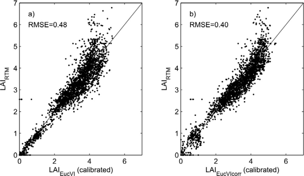
3.1. New Spectral Vegetation Index Calibration

The calibration of Equation 1 using the synthetic PROSAIL database gave the parameters [1, −1.881, 0.001, 0.094, 1.407, 0.018] for EucVI (Table 2). It was possible with this new SVI to approximate the LAI that was obtained by RTM inversion. The difference between the LAI estimated with EucVI and the LAI values obtained from PROSAIL inversion was rather low (RMSE of 0.48; Figure 1(a)). The residual difference illustrates the difficulty of matching the performance of RTM inversion with a single vegetation index, even when calibrated on the same dataset. Many variables not taken into account by the SVI influence the results in the inversion process, like the satellite view angles, the sun angle, etc. Note that Figure 1 does not provide any information on the efficiency of the model to estimate the true Eucalyptus LAI, but indicates how well an SVI can replace a complex RTM inversion procedure. The comparison of LAI estimates and field measurements is presented later (Section 3.2).
The use of age and DoY to correct the EucVI, only slightly improved the results that were already good with EucVI: the RMSE decreased to 0.40 (Figure 1(b)). EucVI and EucVIcorr, are easy to obtain at large scales from the reflectance time series themselves and from the signal acquisition date. The final equation of EucVIcorr is:
EucVI corr = EucVI ( 0.0207 AGE 3 0.1786 AGE 2 + 0.3215 AGE ) ( 1.2 × 10 7 DOY 3 + 5.6 × 10 5 DOY 2 0.0054 DOY ) + 0.0298
with AGE in years and DoY in days. The correction for age and DoY is comprised between −0.45 and +0.6 LAI units, which is rather low and leaves a relatively large scatter in Figure 1(b). The more variables are added to the index, the more the index approaches the original RTM inversion method. However, since the aim of this study was to stay as simple as possible for practical use, the gain of accuracy resulting from these corrections does not seem justified, given that the method using EucVI already gave results close to the RTM inversion methodology (RMSE = 0.48). Note also that the age correction should not be used for ages greater than 6 years which did not occur in our calibration dataset, since rotation length of these Brazilian Eucalyptus plantations is about 6 years. In the following, we however present both results for comparison purposes.

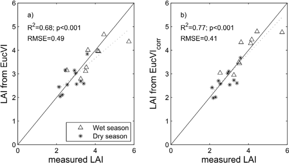
3.2. Comparison with LAI from Destructive Measurements

Figure 2 compares the LAI measured in the field and the LAI estimated from MODIS Red and NIR reflectances, using EucVI and EucVIcorr. The EucVI, which takes the form of Equation (1) parameterized as shown in Table 2, gave a RMSE of 0.49, which is about 15% of the average measured LAI. The EucVIcorr (Equation (2)) index achieved results that approached the performance of the RTM inversion (R2 of 0.77 and RMSE of 0.41, Figure 2(b)). These values can be compared to the R2 of 0.8 and RMSE of 0.41 described in Figure 5 of [14] on the same dataset for the RTM inversion. Note that the destructive LAI measurements and the LAI estimates from EucVI and EucVIcorr are totally independent. Even the regression between the LAI and the SVI (see the point labeled c in introduction) was not calibrated on these field data.
One of the data points is outside the general tendency (Stand SF171 with LAI of 5.7). This high LAI value point, which was well inverted with RTM, is difficult to retrieve with both EucVI and EucVIcorr. This shows one of the advantages of using RTM inversion: it tends to be more precise than EucVIs for high LAI values. This is also visible on Figure 1, where EucVI and LAI from RTM inversion show heteroscedasticity, meaning that the SVI cannot correctly reproduce the LAI inverted with the RTM for high LAI values.
The correlations remained significant when dry and wet season measurements were considered separately, which means that the correlation was not only due to LAI seasonal variations which increase the LAI range, but also to interannual or inter-stand variations for a given season.
Finally, the time-series of LAI retrieved with EucVIcorr are very similar to those obtained with RTM inversion (Figure 3): they show realistic seasonal variations and range of values, as well as good coherence with destructive measurements.

4. Discussion

This study shows that a species-specific SVI can be calibrated from an RTM inversion dataset to take into account most of the variability in canopy biophysical and biochemical properties, their true ranges, distributions and covariance, and the influence of sun and satellite angles. This means that the SVI calibrated with the methodology described in this study is constructed to be as strongly correlated to LAI as possible and therefore to be less sensitive to other canopy variables (SLA, leaf angles, etc.) and to acquisition geometry. Like other generic SVI, our calibrated SVI still has the disadvantage of being specific to its calibration conditions (vegetation, sensor, etc.), but it is easy to test the effect of changes in an RTM parameter (e.g., leaf inclination, chlorophyll content, etc.) on the index, and to calibrate a different index if necessary. Another advantage is that the dataset can represent a broader range of parameters and acquisition geometries than what could be obtained with only LAI field measurements due to the amount of field work involved. For instance, an SVI or an SVI-LAI relationship calibrated at a precise period of the year with field measurements, with a given sun-view configuration or vegetation development stage, cannot be transposed to another period of the year with other properties [39].
The EucVI index parameters show the importance of the Red band as it appears both in the numerator and denominator, with larger coefficients than those of the NIR band. The EucVI coefficients cannot be directly compared to the coefficients of other SVI, since the EucVI is given in the same units as LAI (EucVI = LAI), whereas the SVI-LAI relationship has to be calibrated for other SVI. This is an advantage of the methodology developed in this study, since the field measurements remain totally independent of the index calibration.
A species-specific vegetation index can also be improved by incorporating other variables like stand age or season, as was simply demonstrated in this example on Eucalyptus plantations. The main advantage of the method is that once the index has been calibrated, it can be applied to an entire dataset (classified image, time-series of images, etc.), with considerably more simplicity and efficiency than the RTM inversion technique described in [14]. In the example presented in this study, the performance of the EucVIcorr index was almost equivalent to that of the RTM inversion with which it was calibrated. The SVI presented here used only two wavebands, but other bands could have been added, like the blue band which is taken into account in the EVI index. However, for the particular case of MODIS data used in this study, only Red and NIR bands are provided at 250 m resolution. The other spectral bands are given at 500 m or 1 km resolution, which was insufficient for our study as the large pixels containing the measured stands were not pure Eucalyptus.
The method relies to a large extent on the accuracy of the LAI obtained by RTM inversion, i.e., relies both on the accuracy of the model when simulating the scene in the direct mode [40] and on the accuracy of the RTM inversion method. After this step comes the calibration of the SVI itself. The overall methodology is therefore not simple to implement, but its final result is a species-specific vegetation index that can be used easily and transferred to a community of non-specialist users, while techniques such as model inversion, look up tables, or neural networks will probably mainly remain confidential. In the present case, the EucVIcorr index could be used by plantation managers in a simple integration with GIS-software for near real-time monitoring of stand LAI. However, one must bear in mind that the precision will not be quite as good as that of RTM inversion (in our case a RMSE of 0.49 compared to 0.41 obtained in [14]).
As vegetation maps will become more and more precise in the future, the use of different SVIs depending on the vegetation type or species will be possible for LAI mapping at a regional level. Use of species-specific vegetation indices will improve the estimation of LAI by focusing on the LAI range of interest, avoiding as much as possible other canopy characteristics that may blur the results, and optionally taking into account other variables such as crop age or measurement season. In this study, we insist on the fact that species-specific SVIs should not only rely on different linear or nonlinear models between SVI and LAI, but also on the construction of the SVI itself. In the Brazilian context, EucVI could be used on the more than 4.8 million hectares of Eucalyptus[41]. This index would probably be different from the equivalent SVIs for pasture, sugarcane, orange orchards, corn fields or natural forest, which are the main vegetation types in southeastern Brazil.
The LAI is a very important variable involved in a variety of ecosystem processes. For forest plantations, its estimation over entire rotations (i.e., about 6 to 7 years) is an important step for understanding ecosystem functioning through process-based models. Such models explicitly take into account soil properties and meteorology to simulate gross photosynthesis, autotrophic respiration, allocation, litterfall, etc. They are used routinely by some companies [42]. The LAI is one of the key variables simulated by such models. LAI values retrieved by remote sensing can be compared with model-simulated LAI for model validation reasons, or can be used as a forcing variable in the model. For example, forcing carbon allocation to leaf growth so that simulated LAI matched remotely-sensed “target LAI” improved growth simulations made by the G’Day process-based model [43].

5. Conclusion

We have developed a Eucalyptus-specific spectral vegetation index called EucVI, designed for the easy retrieval of leaf area index (LAI) time series from MODIS reflectance data. The use of a synthetic database, created with a radiative transfer model (RTM) inversion procedure, to calibrate the spectral vegetation indices (SVIs) proved to be an efficient method. It aimed at increasing the number of data points for the calibration process, while still considering “real” cases, i.e., real stands with all the correlations between their biophysical and biochemical properties. The final vegetation index gives good results in most of the LAI range known for Eucalyptus stands in southeastern Brazil. The root mean square error (RMSE) calculated on an independent LAI dataset was 0.49, which is about 15% of the average measured LAI. However, high LAI values are still difficult to retrieve with such an index. The use of age and day of year as easily available additional information in the EucVIcorr index formulation slightly improved the LAI retrieval results (RMSE of 0.41). The indices were tested on a dataset showing a large range of age and soil conditions. However validation on a larger dataset would be useful to confirm their accuracy. This method offers a simple and operational alternative to application of complex and computationally intensive RTM inversion techniques, and could be used to design other species-specific SVIs.

Acknowledgments

This study was funded by the European Integrated Project Ultra Low CO2 Steelmaking (ULCOS—contract no. 515960), by CNPq 306561/2007, and by the EucFlux project. We thank International Paper of Brasil and in particular José Mario Ferreira, Augusto Miguel Nascimento Lima and Sebastião Oliveira, for providing data and technical help for field campaigns and the French Ministry of Foreign Affairs for their financial support. We are also very grateful to Osvaldo Cabral (EMBRAPA), Marcos Ligo (EMBRAPA), Elcio Reis (IPBr), Cristiane Camargo Zani (ESALQ), Giampiero Bini Cano (Instituto Botanico), Renato Meulman Leite da Silva (ESALQ), and Reinaldo Camargo (ESALQ) for their help during field work.

References

  1. Rouse, J.W.; Haas, R.H.; Schell, J.A.; Deering, D.W. Monitoring vegetation systems in the great plains with ERTS. In Third ERTS Symposium, SP-351; Griswold, N., Ed.; NASA: Washington, WA, USA, 1973; Volume 1, pp. 309–317. [Google Scholar]
  2. Jordan, C.F. Derivation of leaf area index from quality of light on the forest floor. Ecology 1969, 50, 663–666. [Google Scholar]
  3. Baret, F.; Clevers, J.G.P.W.; Steven, M.D. The robustness of canopy gap fraction estimates from red and near-infrared reflectances: A comparison of approaches. Remote Sens. Environ 1995, 54, 141–151. [Google Scholar]
  4. Huete, A.R. A Soil-Adjusted Vegetation Index (SAVI). Remote Sens. Environ 1988, 25, 295–309. [Google Scholar]
  5. Justice, C.O.; Vermote, E.; Townshend, J.R.G.; Defries, R.; Roy, D.P.; Hall, D.K.; Salomonson, V.V.; Privette, J.L.; Riggs, G.; Strahler, A.; et al. The Moderate Resolution Imaging Spectroradiometer (MODIS): Land remote sensing for global change research. IEEE Trans. Geosci. Remote Sens 1998, 36, 1228–1249. [Google Scholar]
  6. Huete, A.R.; Liu, H.Q.; Batchily, K.; van Leeuwen, W. A comparison of vegetation indices over a global set of TM images for EOS-MODIS. Remote Sens. Environ 1997, 59, 440–451. [Google Scholar]
  7. Brown, L.; Chen, J.M.; Leblanc, S.G.; Cihlar, J. A shortwave infrared modification to the simple ratio for LAI retrieval in boreal forests: An image and model analysis. Remote Sens. Environ 2000, 71, 16–25. [Google Scholar]
  8. Fassnacht, K.S.; Gower, S.T.; MacKenzie, M.D.; Nordheim, E.V.; Lillesand, T.M. Estimating the leaf area index of North Central Wisconsin forests using the landsat thematic mapper. Remote Sens. Environ 1997, 61, 229–245. [Google Scholar]
  9. Qi, J.; Kerr, Y.H.; Moran, M.S.; Weltz, M.; Huete, A.R.; Sorooshian, S.; Bryant, R. Leaf area index estimates using remotely sensed data and BRDF models in a semiarid region. Remote Sens. Environ 2000, 73, 18–30. [Google Scholar]
  10. Propastin, P.A. Spatial non-stationarity and scale-dependency of prediction accuracy in the remote estimation of LAI over a tropical rainforest in Sulawesi, Indonesia. Remote Sens. Environ 2009, 113, 2234–2242. [Google Scholar]
  11. Yoshioka, H.; Miura, T.; Obata, K. Derivation of relationships between spectral vegetation indices from multiple sensors based on vegetation isolines. Remote Sens 2012, 4, 583–597. [Google Scholar]
  12. Soudani, K.; Francois, C.; le Maire, G.; Le Dantec, V.; Dufrene, E. Comparative analysis of IKONOS, SPOT, and ETM+ data for leaf area index estimation in temperate coniferous and deciduous forest stands. Remote Sens. Environ 2006, 102, 161–175. [Google Scholar] [Green Version]
  13. Jackson, R.D.; Huete, A.R. Interpreting vegetation indices. Prev. Vet. Med 1991, 11, 185–200. [Google Scholar]
  14. le Maire, G.; Marsden, C.; Verhoef, W.; Ponzoni, F.J.; Lo Seen, D.; Bégué, A.; Stape, J.-L.; Nouvellon, Y. Leaf area index estimation with MODIS reflectance time series and model inversion during full rotations of Eucalyptus plantations. Remote Sens. Environ 2011, 115, 586–599. [Google Scholar]
  15. Verrelst, J.; Romijn, E.; Kooistra, L. Mapping vegetation density in a heterogeneous river floodplain ecosystem using pointable CHRIS/PROBA data. Remote Sens 2012, 4, 2866–2889. [Google Scholar]
  16. Gilabert, M.A.; Gonzalez-Piqueras, J.; Garcia-Haro, F.J.; Melia, J. A generalized soil-adjusted vegetation index. Remote Sens. Environ 2002, 82, 303–310. [Google Scholar]
  17. Campoe, O.C.; Stape, J.L.; Nouvellon, Y.; Laclau, J.-P.; Bauerle, W.; Binkley, D.; le Maire, G. Stem production, light absorption and light use efficiency between dominant and non-dominant trees of Eucalyptus grandis across a productivity gradient in Brazil. For. Ecol. Manage 2012, 288, 14–20. [Google Scholar]
  18. Nouvellon, Y.; Laclau, J.-P.; Epron, D.; Kinana, A.; Mabiala, A.; Roupsard, O.; Bonnefond, J.-M.; le Maire, G.; Marsden, C.; Bontemps, J.-D.; et al. Within-stand and seasonal variations of specific leaf area in a clonal Eucalyptus plantation in the Republic of Congo. For. Ecol. Manage 2010, 259, 1796–1807. [Google Scholar]
  19. Gower, S.T.; Kucharik, C.J.; Norman, J.M. Direct and indirect estimation of leaf area index, fAPAR, and net primary production of terrestrial ecosystems. Remote Sens. Environ 1999, 70, 29–51. [Google Scholar]
  20. MacFarlane, C.; Arndt, S.K.; Livesley, S.J.; Edgar, A.C.; White, D.A.; Adams, M.A.; Eamus, D. Estimation of leaf area index in eucalypt forest with vertical foliage, using cover and fullframe fisheye photography. For. Ecol. Manage 2007, 242, 756–763. [Google Scholar]
  21. Wolfe, R. MODIS Geolocation. In Earth Science Satellite Remote Sensing; Springer: Berlin/Heidelberg, Germany, 2006; Volume 1, pp. 50–73. [Google Scholar]
  22. Feret, J.-B.; François, C.; Asner, G.P.; Gitelson, A.A.; Martin, R.E.; Bidel, L.P.R.; Ustin, S.L.; le Maire, G.; Jacquemoud, S. PROSPECT-4 and 5: Advances in the leaf optical properties model separating photosynthetic pigments. Remote Sens. Environ 2008, 112, 3030–3043. [Google Scholar]
  23. Jacquemoud, S.; Baret, F.; Hanocq, J.F. Modeling spectral and bidirectional soil reflectance. Remote Sens. Environ 1992, 41, 123–132. [Google Scholar]
  24. Verhoef, W.; Bach, H. Coupled soil-leaf-canopy and atmosphere radiative transfer modeling to simulate hyperspectral multi-angular surface reflectance and TOA radiance data. Remote Sens. Environ 2007, 109, 166–182. [Google Scholar]
  25. Baret, F.; Guyot, G. Potentials and limits of vegetation indices for LAI and APAR assesment. Remote Sens. Environ 1991, 35, 161–173. [Google Scholar]
  26. Clevers, J.G.P.W.; Verhoef, W. LAI estimation by means of the WDVI: A sensitivity analysis with a combined PROSPECT-SAIL model. Remote Sens. Rev 1993, 7, 43–64. [Google Scholar]
  27. Rondeaux, G.; Steven, M.; Baret, F. Optimization of soil-adjusted vegetation indices. Remote Sens. Environ 1996, 55, 95–107. [Google Scholar]
  28. Jiang, Z.; Huete, A.R.; Didan, K.; Miura, T. Development of a two-band enhanced vegetation index without a blue band. Remote Sens. Environ 2008, 112, 3833–3845. [Google Scholar]
  29. Peterson, D.L.; Spanner, M.A.; Running, S.W.; Teuber, K.B. Relationship of thematic mapper simulator data to leaf area index of temperate coniferous forests. Remote Sens. Environ 1987, 22, 323–341. [Google Scholar]
  30. Turner, D.P.; Cohen, W.B.; Kennedy, R.E.; Fassnacht, K.S.; Briggs, J.M. Relationships between leaf area index and Landsat TM spectral vegetation indices across three temperate zone sites. Remote Sens. Environ 1999, 70, 52–68. [Google Scholar]
  31. Tucker, C.J. Red and photographic infrared linear combinations for monitoring vegetation. Remote Sens. Environ 1979, 8, 127–150. [Google Scholar]
  32. Crippen, R.E. Calculating the vegetation index faster. Remote Sens. Environ 1990, 34, 71–73. [Google Scholar]
  33. Clevers, J.G.P.W. Application of a weighted infrared-red vegetation index for estimating leaf area index by correcting for soil moisture. Remote Sens. Environ 1989, 29, 25–37. [Google Scholar]
  34. Richardson, A.J.; Wiegand, C.L. Distinguishing vegetation from soil background information. Photogramm. Eng. Remote Sensing 1977, 43, 1541–1552. [Google Scholar]
  35. le Maire, G.; François, C.; Soudani, K.; Berveiller, D.; Pontailler, J.-Y.; Bréda, N.; Genet, H.; Davi, H.; Dufrêne, E. Calibration and validation of hyperspectral indices for the estimation of broadleaved forest leaf chlorophyll content, leaf mass per area, leaf area index and leaf canopy biomass. Remote Sens. Environ 2008, 112, 3846–3864. [Google Scholar]
  36. le Maire, G.; Francois, C.; Dufrene, E. Towards universal broad leaf chlorophyll indices using PROSPECT simulated database and hyperspectral reflectance measurements. Remote Sens. Environ 2004, 89, 1–28. [Google Scholar]
  37. Press, W.; Teukolsky, S.; Vetterling, W.; Flannery, B. Numerical Recipes in Fortran 77, 2nd ed.; Cambridge University Press: New York, NY, USA, 1996. [Google Scholar]
  38. le Maire, G.; Marsden, C.; Nouvellon, Y.; Grinand, C.; Hakamada, R.; Stape, J.-L.; Laclau, J.-P. MODIS NDVI time-series allow the monitoring of Eucalyptus plantation biomass. Remote Sens. Environ 2011, 115, 2613–2625. [Google Scholar]
  39. Wang, Q.; Adiku, S.; Tenhunen, J.; Granier, A. On the relationship of NDVI with leaf area index in a deciduous forest site. Remote Sens. Environ 2005, 94, 244–255. [Google Scholar]
  40. Atzberger, C.; Darvishzadeh, R.; Schlerf, M.; le Maire, G. Suitability and adaptation of PROSAIL radiative transfer model for hyperspectral grassland studies. Remote Sens. Lett 2013, 4, 55–64. [Google Scholar]
  41. Brazilian Association of Forest Plantation Producers. Chapter 1 Planted forests in Brazil. Statistical Yearbook. 2012. Available online: http://www.abraflor.org.br/estatisticas/ABRAF12/ABRAF12-EN.pdf (accessed on 20 September 2012).
  42. Almeida, A.C.; Landsberg, J.J.; Sands, P.J.; Ambrogi, M.S.; Fonseca, S.; Barddal, S.M.; Bertolucci, F.L. Needs and opportunities for using a process-based productivity model as a practical tool in Eucalyptus plantations. For. Ecol. Manage 2004, 193, 167–177. [Google Scholar]
  43. le Maire, G.; Marsden, C.; Laclau, J.-P.; Stape, J.-L.; Corbeels, M.; Nouvellon, Y. Spatial and Temporal Variability of the Carbon Budget of Tropical Eucalyptus Plantations Assessed Using Ecosystem Modelling and Remote Sensing. Proceedings of Landmod 2010: International Conference on Integrative Landscape Modelling, Montpellier, France, 3–5 February 2010; pp. 1–8.
Figure 1. (a) Results of the calibration of EucVI: Parameters of Equation 1 were estimated by minimizing the RMSE between LAI estimated from EucVI (LAIEucVI) and LAI estimated by RTM inversion (LAIRTM). (b) Results of the calibration of EucVIcorr which takes into account age and DoY (Equation (2)). The data consist of 2620 LAI estimates obtained by RTM inversion, using Red and NIR MODIS reflectances of 18 different stands of different ages and soil conditions, from their planting date up to year 2009.
Remotesensing 04 03766f1
Figure 2. Comparison of measured (by destructive sampling) LAI and LAI estimated from (a) EucVI and (b) EucVIcorr. These results can also be compared with those of PROSAIL inversion and of the GESAVI index in [14].
Remotesensing 04 03766f2
Figure 3. LAI time-series on the nine stands of Table 1, since the beginning of the rotation. The black line represents the results of the RTM inversion [14], the red line those of the EucVIcorr index, and black stars indicate LAI values obtained from destructive measurements.
Remotesensing 04 03766f3
Table 1. Description of the nine Eucalyptus stands where leaf area index (LAI) was measured (using a “destructive” methodology). The LAI measurements were used for validation purposes. DOY: day of year; D.S: dry season; W.S.: wet season.
Stand NameArea (ha)Plantation DateAge on 1 April 2009 (yr)Date of LAI Measurements (DOY)LAI (m2·m−2)
D.S. 2007W.S. 2008D.S. 2008W.S. 2009D.S. 2007W.S. 2008D.S. 2008W.S. 2009
SF183U108.2703/04/20072942603.52.3
SF178U93.1229/03/20063.01932624.42.9
NS24U108.5304/04/200632553.6
SF17148.705/05/20053.91932605.73.0
SF43E65.5206/05/20044.91912634.23.4
MG14U37.1326/03/20045.022542.2
SF8940.3111/06/20035.81952603.52.3
IT14006/03/20036.0833293282213.24.13.03.5
IT216006/03/20036.0833293282212.63.62.13.2
Table 2. Examples of classical 2-band (RED and NIR) spectral vegetation indices, and SVI calibrated for Eucalyptus (GESAVI cal and EucVI). Values of parameters [a, b, c, d, e, f] refer to the parameters of Equation 1. Other letters correspond to the variables described below the table.
SVIReferenceabcdef
DVI[31]1−10001
NDVI[1]1−10110
IPVI[32]100110
RVI[2]100010
WDVI(1)[33]1−A0001
PVI(1)[34]1−A−B00 1 + A 2
SAVI(2)[4](1 + L)−(1 + L)011L
TSAVI(1,3)[25]A−A2−A × BA1−A × B + X(1 + A2)
OSAVI(4)[27]1−1011Y
EVI2(5)[28]G−G016 – 7.5/C1
GESAVI(1,6)[16]1−A−B01Z
GESAVI(7)[14]1−1.505−0.034010.0383
EucVI(8)This study1−1.8810.0010.0941.4070.018
(1)A is the slope of the soil line in (RED, NIR) space, B is the intercept;
(2)L is a parameter varying between 0 and 1 depending on the vegetation amount, Standard value L = 0.5;
(3)X is a parameter which can vary, standard value X = 0.08;
(4)Y is a soil adjustment coefficient, standard value Y = 0.16;
(5)C is a parameter such that Red = C × Blue, G is adjusted, standard value C = 2.08 and G = 2.5;
(6)Z is a parameter, standard value Z = 0.35;
(7)The parameters A, B and Z of GESAVI were estimated for Eucalyptus plantations on MODIS reflectance;
(8)Parameter a was fixed to 1.

