A Comparison between Local and Global Spaceborne Chlorophyll Indices in the St. Lawrence Estuary


 , ,
, ,
Abstract
:1. Introduction
2. Materials and Methods
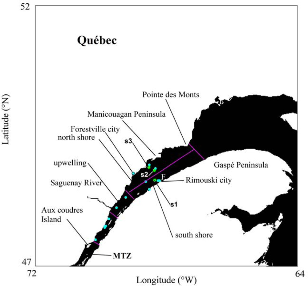
2.1. Field Surveys
2.2. Lab Analysis of Optical Variables
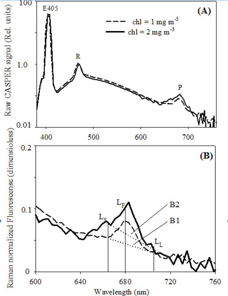
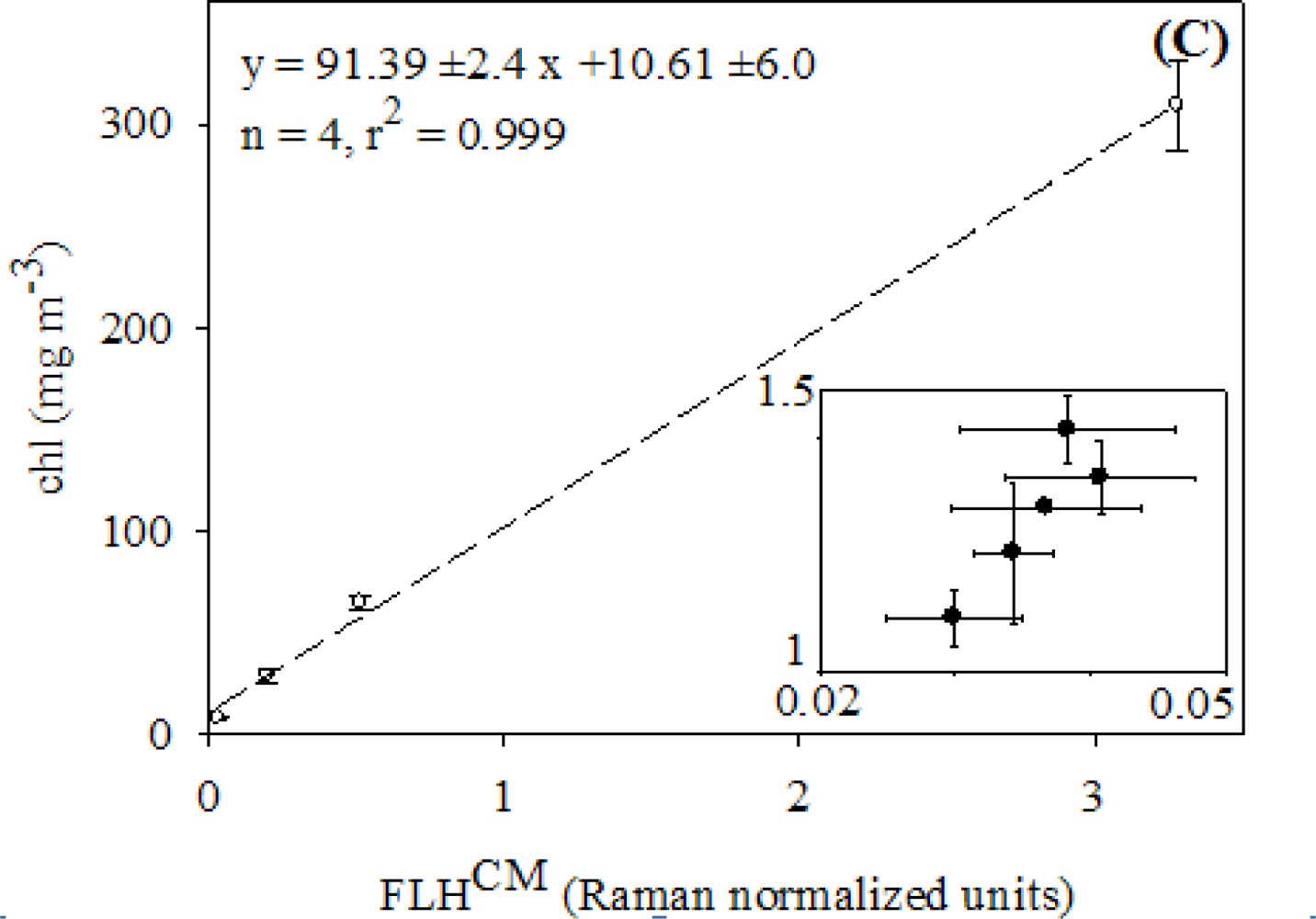
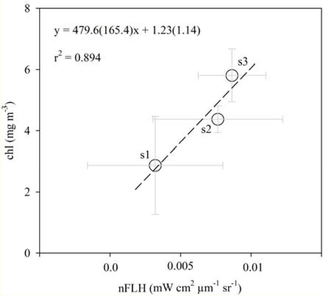
2.3. Relationships between FLH and Chlorophyll
2.4. Satellite Ocean Color Measurements
2.4.1. Datasets
2.4.2. Analysis of Imagery
2.4.3. Statistical Analysis
3. Results
3.1. Relationships between chl and FLH as Derived from Field and Lab Samples
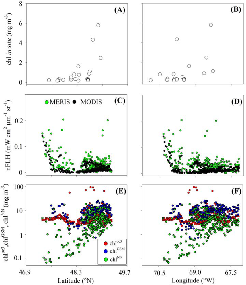
3.2. Chlorophyll Proxies Based on Satellite-Derived FLH and Lw
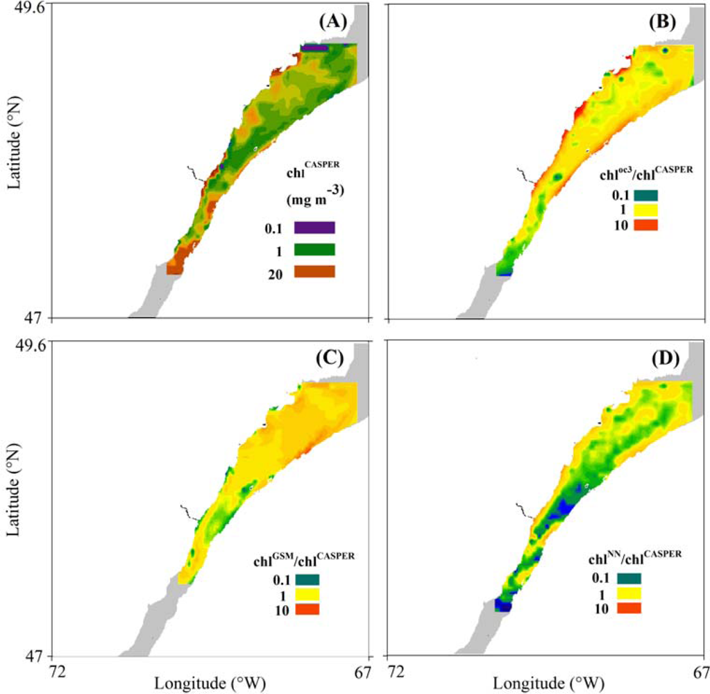
3.3. Spatial Coherence between Fluorescence and Lw-Based Indices of chl
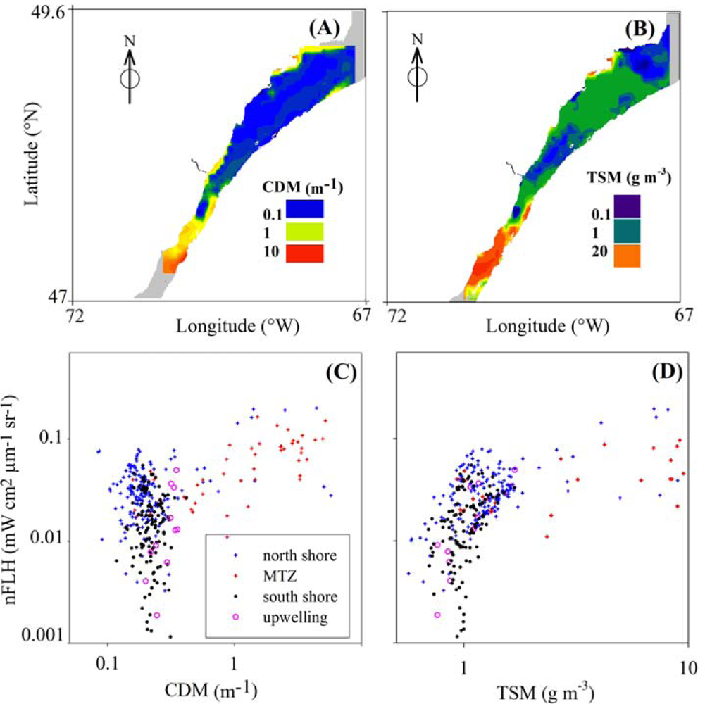
3.4. Effects of CDOM and Detritus on FLH
4. Discussion
4.1. Relationships between chl and CASPER Fluorescence
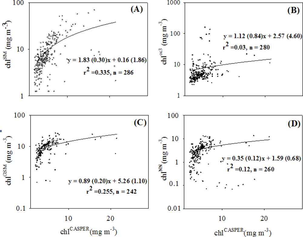
4.2. Coherence between chlCASPER and other Chlorophyll Indices
4.3. Spatial Distribution of Spaceborne Chl Indices
5. Conclusions
Acknowledgments
References
- Legendre, L. The significance of microalgal blooms for fisheries and for the export of particulate organic carbon in oceans. J. Plankton Res 1990, 12, 681–699. [Google Scholar]
- Fauchot, J.; Saucier, F.J.; Levasseur, M; Roy, S; Zakardjian, B. Wind-driven river plume dynamics and toxic Alexandrium tamarense blooms in the St. Lawrence estuary (Canada): A modeling study. Harmful Algae 2008, 7, 214–227. [Google Scholar]
- Montes-Hugo, M.; Carder, K.; Foy, R.; Cannizzaro, J.; Brown, E.; Pegau, S. Estimating phytoplankton biomass in coastal waters of Alaska using airborne remote sensing. Remote Sens. Environ 2005, 98, 481–493. [Google Scholar]
- McKee, D.; Cunningham, A.; Dudek, A. Optical water type discrimination and tuning remote sensing band-ratio algortihms: Application to retrieval of chlorophyll and Kd(490) in the Irish and Celtic Seas. Estuar. Coast. Shelf Sci 2007, 73, 827–834. [Google Scholar]
- Carder, K.; Chen, F.R.; Lee, Z.P.; Hawes, S.K.; Kamykowski, D. Semianalytic Moderate-Resolution Imaging Spectrometer Algorithms for Chlorophyll A and Absorption with bio-optical domains based on nitrate-depletion temperatures. J. Geoph. Res.-Oceans 1999, 104, 5403–5421. [Google Scholar]
- Letelier, R.M.; Abbott, M.R. An analysis of chlorophyll fluorescence algorithms for the Moderate Resolution Imaging Spectrometer (MODIS). Remote Sens. Environ 1996, 58, 215–223. [Google Scholar]
- Montes-Hugo, M.A.; Mohammadpour, G. Biogeo-optical modeling of SPM in the St Lawrence Estuary. Can. J. Remote Sens 2012, 38, 1–13. [Google Scholar]
- Gower, J.F.R. Study of Fluorescence-Based Chlorophyll a Concentration Algorithms for Case 1 and Case 2 Waters; European Space Agency (ESA), European Space Research and Technology Centre (ESTEC): Noordwijk, The Netherlands, 1999; Contract 12295/97/NL/RE. [Google Scholar]
- Gilerson, A.; Zhou, J.; Hlaing, S.; Iannou, I.; Schalles, J.; Gross, B.; Moshary, F.; Ahmed, S. Fluorescense component in the reflectance spectra from coastal waters. Dependence on water composition. Opt. Exp 2007, 15, 15702–15721. [Google Scholar]
- Abbott, M.R.; Letelier, R.M. Algorithm Theoretical Basis Document. Chlorophyll Fluorescence (MODIS Product Number 20); NASA: Pasadena, MD, USA, 1999; p. 42. [Google Scholar]
- Nieke, B.; Reuter, R.; Heuermann, R.; Wang, H.; Babin, M.; Therriault, J.C. Light absorption and fluorescence properties of chromophoric dissolved organic matter (CDOM) in the St. Lawrence Estuary (Case 2 waters). Cont. Shelf Res 1997, 17, 235–252. [Google Scholar]
- D’Anglejan, B.F.; Smith, E.C. Distribution, transport and composition of suspended matter in the St. Lawrence Estuary. Can. J. Earth Sci 1973, 10, 1380–1396. [Google Scholar]
- Fuentes-Yaco, C.; Vezina, A.F.; Larouche, P; Vigneau, C; Gosselin, M; Levasseur, M. Phytoplankton pigment in the Gulf of St. Lawrence, Canada, as determined by the Coastal Zone Color Scanner. Part 1. Spatio-temporal variability. Cont. Shelf Res 1997, 17, 1421–1439. [Google Scholar]
- Mucci, A.; Starr, M.; Gilbert, D.; Sundby, B. Acidification of the lower St Lawrence Estuary bottom waters. Atmosphere-Ocean 2011, 49, 206–218. [Google Scholar]
- Trees, C.C.; Bidigare, R.R.; Karl, D.M.; Van Heukelem, L. Fluorometric Chlorophyll a: Sampling, Laboratory, Methods and Data Analysis Protocols. In Ocean Optics Protocols for Satellite Ocean Color Sensor Validation; Chapter 14, Revision 2; NASA Report; Goddard Space Flight Space Center: Greenbelt, MD, USA, 2000. [Google Scholar]
- Colao, F.; Demetrio, E.; Drozdowska, V.; Fiorani, L.; Lazi, V.; Okladnikov, I.; Palucci, A. Seawater Dual Fluorescence Analysis during the Arctic Summer 2006 Polish Oceanographic Campaign. Proceedings of 3rd EARSel Workshop Remote Sensing of the Coastal Zone, Bolzano, Italy, 7–9 June 2007.
- Falkowski, P.G.; Kiefer, D.A. Chlorophyll a fluorescence in phytoplankton: relationship to photosynthesis and biomass. J. Plankton Res 1985, 7, 715–731. [Google Scholar]
- Neville, R.A.; Gower, J.F.R. Passive remote sensing of phytoplankton via chlorophyll fluorescence. J. Geophys. Res 1977, 82, 3487–3493. [Google Scholar]
- Borstad, G.A.; Edel, H.R.; Gower, J.F.R.; Hollinger, A.B. Analysis of Test and Flight Data from the Fluorescence Line Imager. In Can. Spec. Publ. Fish. Aquat. Sci.; Canada Dept. of Fisheries and Oceans: Ottawa, ON, Canada, 1985; Volume 83, p. 48. [Google Scholar]
- Gower, J.F.R; Brown, L.; Borstad, G.A. Observation of chlorophyll fluorescence in west coast waters of Canada using the MODIS satellite sensor. Can. J. Remote Sens 2004, 30, 17–25. [Google Scholar]
- Ocean Color Web. Available online: http://oceancolor.gsfc.nasa.gov/ (accessed on 1 January 2012).
- GlobColour. Available online: http://hermes.acri.fr/ (accessed on 1 January 2012).
- O’Reilly, J.E.; Maritorena, S.; Mitchell, B.G.; Siegel, D.A.; Carder, K.L.; Garver, S.A.; Karhu, M.; Garver, S.A.; MCClain, S.A. Ocean color algorithms for SeaWiFS. J. Geoph. Res 1998, 103, 24937–24953. [Google Scholar]
- Maritorena, S.; Siegel, D.A. Consistent merging of satellite ocean color data sets using a bio-optical model. Remote Sens. Environ 2005, 94, 429–440. [Google Scholar]
- Doerffer, R.; Schiller, H. The MERIS Case 2 algorithm. Int. J. Remote Sens 2007, 28, 517–535. [Google Scholar]
- Doerffer, R.; Schiller, H. MAPP Data Products Definition and Algorithm Specification. Algorithm Theoretical Basis Document (ATBD). Regionalized Case II Water Products and Algorithms; ATBD 1, Report; GKSS Research Center: Hamburg, Germany, 2000; p. 87. [Google Scholar]
- Behrenfeld, M.; Westberry, T.K.; Boss, E.S.; O’Malley, R.T.; Siegel, D.A.; Wiggert, J.D.; Franz, B.A.; McClain, C.R.; Feldman, G.C.; Doney, S.C.; Moore, J.K.; Dall’Olmo, G.; Milligan, A.G.; Lima, I; Mahowald, N. Satellite-detected fluorescence reveals global physiology of ocean phytoplankton. Biogeosciences 2009, 6, 779–794. [Google Scholar]
- Gordon, H.R.; Clark, D.K. Clear water radiances for atmospheric correction of coastal zone color scanner imagery. Appl. Opt 1981, 20, 4175–4180. [Google Scholar]
- GlobProject. Available online: http://www.brockmann-consult.de (accessed on 1 January 2012).
- Windows Image Manager Software. Available online: http://wimsoft.com/ (accessed on 1 January 2012).
- Sokal, R.R.; Rohlf, F.J. Biometry; W.H. Freeman: New York, NY, USA, 1995; p. 498. [Google Scholar]
- Pearson, R.K. Mining Imperfect Data. Dealing with Contamination and Incomplete Records; Society for Industrial and Applied Mathematics: Philadelphia, PA, USA, 2005; p. 305. [Google Scholar]
- Gilerson, A.; Zhou, J.; Hlaing, S.; Iannou, I.; Gross, B.; Moshary, F.; Ahmed, S. Fluorescence component in the reflectance spectra from coastal waters. II. Performance of retrieval algorithms. Opt. Exp 2007, 16, 2446–2460. [Google Scholar]
- Ahn, Y-H; Shanmugam, P. Derivation and analysis of the fluorescence algorithms to estimate phytoplankton pigment concentration in optically complex coastal waters. J. Opt. A-Pure Appl. Opt 2007, 9, 352–362. [Google Scholar]
- Welschmeyer, N.A. Fluorometric analysis of chlorophyll a in the presence of chlorophyll b and phaeopigments. Limnol. Oceanogr 1994, 39, 1985–1992. [Google Scholar]
- Mas, S. Le Rôle du Phytoplancton de petite Taille (<20 μm) dans les Variations des Propriétés Optiques des Eaux du Saint-Laurent. Université du Québec a Rimouski, Rimouski, QC, Canada, 2008; p. 286. [Google Scholar]
- Cloern, J.E.; Grenz, C.; Vidergar-Lucas, L. An empirical model of the phytoplankton chlorophyll: Carbon ratio-the conversion factor between productivity and growth rate. Limnol. Oceanogr 1995, 40, 1313–1321. [Google Scholar]
- Poryvkina, L.; Babichenko, S.; Leeben, A. Analysis of Phytoplankton Pigments by Excitation Spectra of Fluorescence. Proceedings of EARsel-SIG Workshop, Lidar Remote Sensing of Land and Sea, Dresden, Germany, 16–17 June 2000.
- Roy, S.; Chanut, J.P.; Gosselin, M.; Sime-Ngando, T. Characterization of phytoplankton communities in the lower St Lawrence Estuary using HPLC-detected pigments and cell microscopy. Mar. Ecol. Progr. Ser 1996, 142, 55–73. [Google Scholar]
- Levasseur, M.; Therriault, J.C.; Legendre, L. Hiercharchid controls of phytoplankton succession by physical factors. Mar. Ecolo. Progr.Ser 1984, 19, 211–222. [Google Scholar]
- Lucotte, M. Organic carbon isotope ratios and implications for the maximum turbidity zone of the St Lawrence Estuary. Est. Coast. Shelf Sci 1989, 29, 293–304. [Google Scholar]
- Fortier, L.; Leggett, W.C. A drift study of larval fish survival. Mar. Ecol. Progr. Ser 1985, 25, 245–257. [Google Scholar]
- Therriault, J.-C.; Levasseur, M. Control of phytoplankton production in the lower St. Lawrence Estuary: Light and freshwater run-off. Le Nat. Canad 1985, 112, 77–96. [Google Scholar]
- Vermote, E.F.; El Saleous, N.Z.; Justice, C.O. Atmospheric correction of MODIS data in the visible to middle infrared: first results. Remote Sens. Environ 2002, 83, 97–111. [Google Scholar]
- Roy, S.; Blouin, F.; Jacques, A.; Therriault, J.C. Absorption properties of phytoplankton in the lower Estuary and Gulf of St Lawrence. Can. J. Fish. Aquat. Sci 2008, 65, 1721–1737. [Google Scholar]
- Montes-Hugo, M.; Mohammadpour, G. Uncertainties on satellite-derived SPM estimates due to bottom–reflected light: A case study in the Saint Lawrence Estuary. Int. J. App. Earth Obs. Geoinf. 2012. submitted.. [Google Scholar]


| Abbreviation | Definition | Units |
|---|---|---|
| Lw | water leaving radiance | mW·cm−2·μm−1·sr−1 |
| nLw | Normalized Lw or Lw assuming sun at zenith and no atmosphere | mW·cm−2·μm−1·sr−1 |
| Rrs | Remote sensing reflectance | sr−1 |
| FLH | Fluorescence line height | mW·cm−2·μm−1·sr−1 |
| FLHCM | Raman-normalized FLH as derived from CASPER | mW·cm−2·μm−1·sr−1 |
| nFLH | Normalized FLH or FLH computed using nLw | mW·cm−2·μm−1·sr−1 |
| aph | Light absorption coefficient of phytoplankton | m−1 |
| ΦF | Quantum yield of fluorescence | dimensionless |
| chlSM | Chlorophyll concentration as derived from ship and MODIS measurements | mg·m−3 |
| chlCASPER | Chlorophyll concentration as derived from MERIS data and CASPER-derived FLH relationship | mg·m−3 |
| chloc3 | Chlorophyll concentration computed using the oc3 model | mg·m−3 |
| chlGSM | Chlorophyll concentration computed using the Garver-Siegel-Maritorena model | mg·m−3 |
| chlNN | Chlorophyll concentration computed using the neural network model | mg·m−3 |
| CDOM | Chromophoric dissolved organic matter | m−1 |
| CDM | CDOM absorption coefficient at 443 nm | m−1 |
| TSM | total suspended matter concentration | g·m−3 |
| MTZ | Maximum turbidity zone |
| k1 | k2 | r2 | N | |
|---|---|---|---|---|
| chlSM | 109.3 | 51.81 | 0.35 | 286 |
| 55.5 | 30.46 | |||
| chloc3 | 33.51 | 14.57 | 0.03 | 280 |
| 28.80 | 17.50 | |||
| chlGSM | 27.85* | 8.58* | 0.37 | 242 |
| 3.63 | 1.82 | |||
| chlNN | 9.99* | 9.15* | 0.18 | 260 |
| 2.36 | 3.52 |
Share and Cite
Montes-Hugo, M.A.; Fiorani, L.; Marullo, S.; Roy, S.; Gagné, J.-P.; Borelli, R.; Demers, S.; Palucci, A. A Comparison between Local and Global Spaceborne Chlorophyll Indices in the St. Lawrence Estuary. Remote Sens. 2012, 4, 3666-3688. https://doi.org/10.3390/rs4123666
Montes-Hugo MA, Fiorani L, Marullo S, Roy S, Gagné J-P, Borelli R, Demers S, Palucci A. A Comparison between Local and Global Spaceborne Chlorophyll Indices in the St. Lawrence Estuary. Remote Sensing. 2012; 4(12):3666-3688. https://doi.org/10.3390/rs4123666
Chicago/Turabian StyleMontes-Hugo, Martin A., Luca Fiorani, Salvatore Marullo, Suzanne Roy, Jean-Pierre Gagné, Rodolfo Borelli, Serge Demers, and Antonio Palucci. 2012. "A Comparison between Local and Global Spaceborne Chlorophyll Indices in the St. Lawrence Estuary" Remote Sensing 4, no. 12: 3666-3688. https://doi.org/10.3390/rs4123666