A Web Platform Development to Perform Thematic Accuracy Assessment of Sugarcane Mapping in South-Central Brazil

Abstract
:1. Introduction
2. Materials and Methods
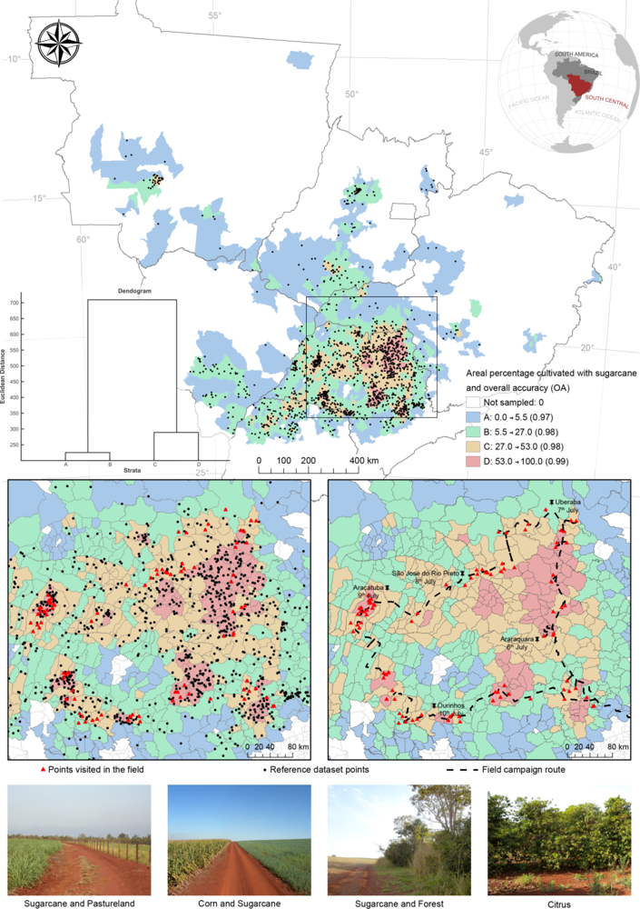
2.1. Statistical Design
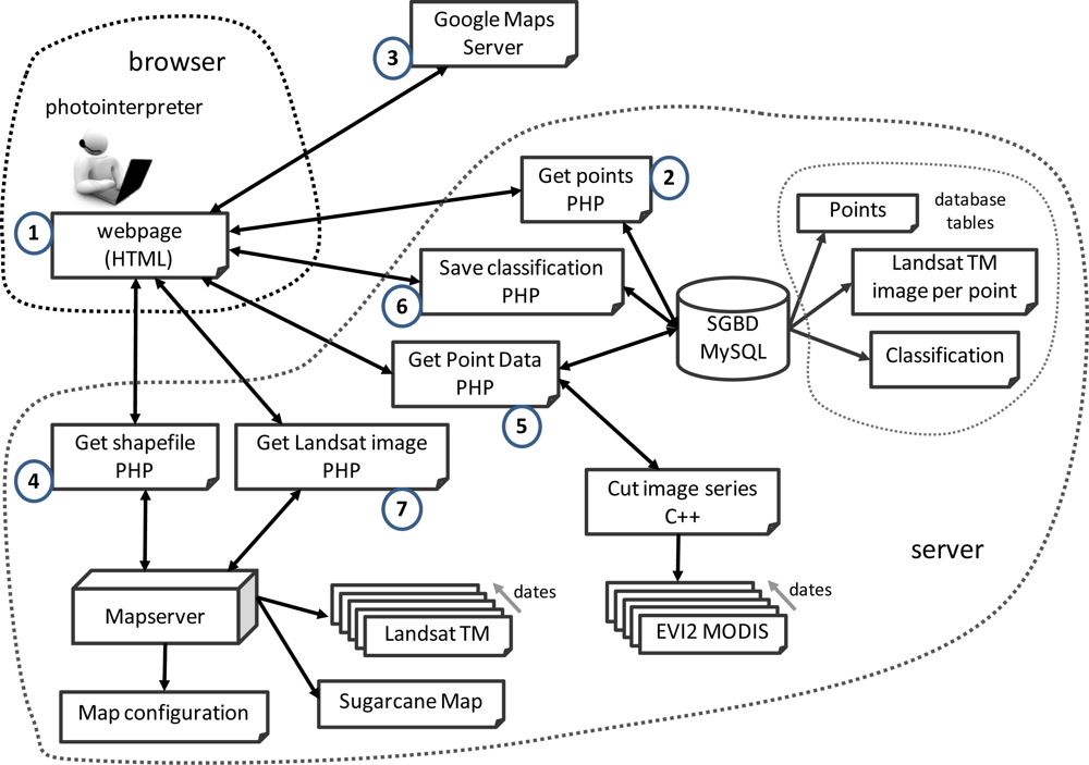
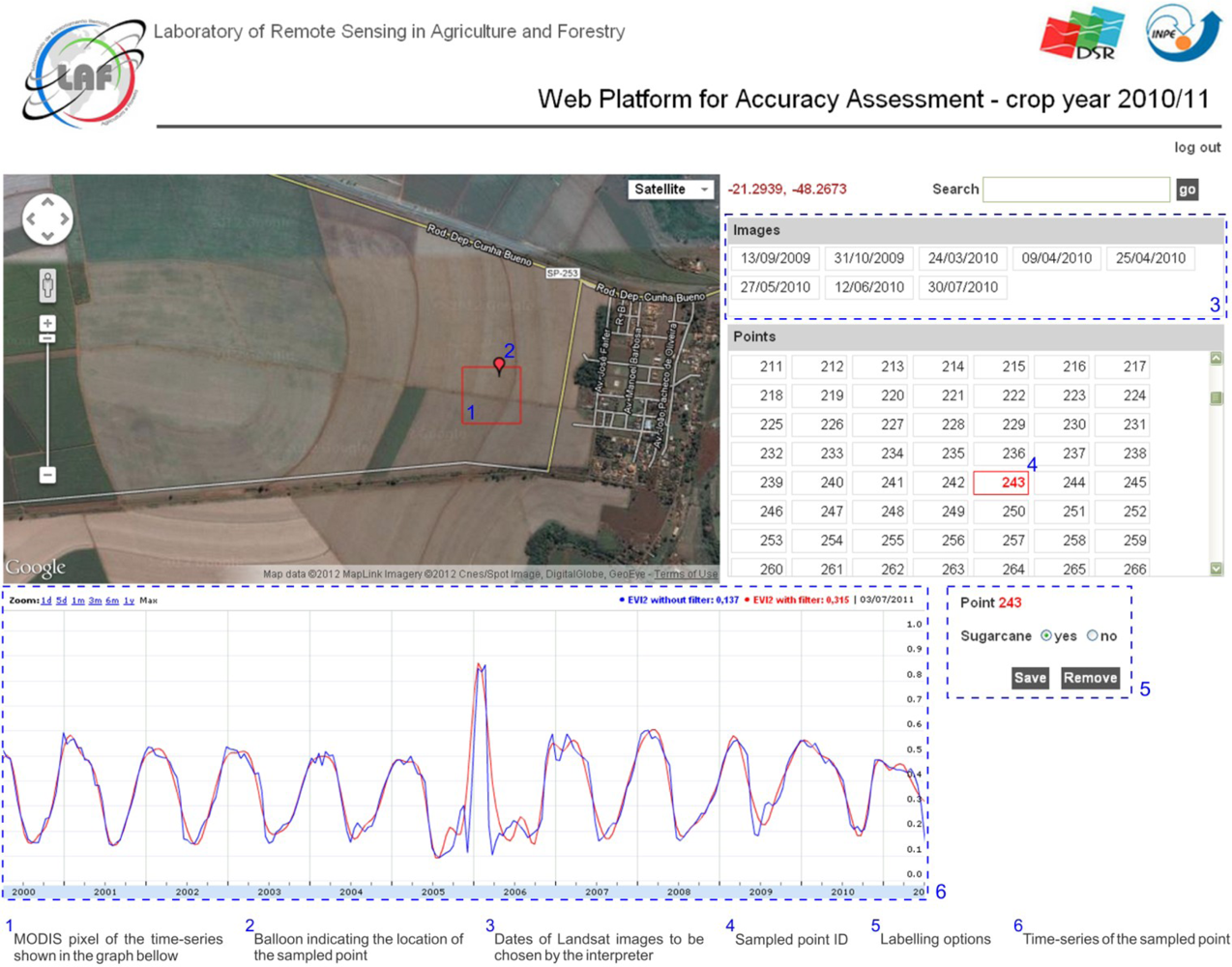
2.2. Web Platform and Reference Database
3. Results and Discussion
4. Summary and Final Considerations
Acknowledgments
References
- FAO (Food and Agriculture Organization of the United Nation). FAOSTAT: FAO Statistical Database. Available online: http://faostat.fao.org (accessed on 9 April 2012).
- IBGE (Instituto Brasileiro de Geografia e Estatística). Sistema IBGE de Recuperação Automática (SIDRA). Available online: http://www.sidra.ibge.gov.br (accessed on 20 January 2012).
- Goldemberg, J. Ethanol for a sustainable energy future. Science 2007, 315, 808–810. [Google Scholar]
- Leite, R.C.C.; Leal, M.R.L.V.; Cortez, L.A.B.; Griffin, W.M.; Scandiffio, M.I.G. Can Brazil replace 5% of the 2025 gasoline world demand with ethanol? Energy 2009, 34, 655–661. [Google Scholar]
- Macedo, I.C.; Seabra, J.E.A.; Silva, J.E.A.R. Green house gases emissions in the production and use of ethanol from sugarcane in Brazil: The 2005/2006 averages and a prediction for 2020. Biomass Bioener 2008, 32, 582–595. [Google Scholar]
- Kim, H.; Kim, S.; Dale, B.E. Biofuels, land use change, and greenhouse gas emissions: Some unexplored variables. Environ. Sci. Technol 2009, 43, 961–967. [Google Scholar]
- Figueiredo, E.B.; La Scala, N., Jr. Greenhouse gas balance due to the conversion of sugarcane areas from burned to green harvest in Brazil. Agr. Ecosyst. Environ 2011, 141, 77–85. [Google Scholar]
- Rudorff, B.F.T.; Aguiar, D.A.; Silva, W.F.; Sugawara, L.M.; Adami, M.; Moreira, M.A. Studies on the rapid expansion of sugarcane for ethanol production in São Paulo State (Brazil) using Landsat data. Remote Sens 2010, 2, 1057–1076. [Google Scholar]
- Aguiar, D.A.; Rudorff, B.F.T.; Silva, W.F.; Adami, M.; Mello, M.P. Remote sensing images in support of environmental protocol: Monitoring the sugarcane harvest in São Paulo State, Brazil. Remote Sens 2011, 3, 2682–2703. [Google Scholar]
- Adami, M.; Rudorff, B.F.T.; Freitas, R.M.; Aguiar, D.A.; Sugawara, L.M.; Mello, M.P. Remote sensing time series to evaluate direct land use change of recent expanded sugarcane crop in Brazil. Sustainability 2012, 4, 574–585. [Google Scholar]
- Nassar, A.M.; Rudorff, B.F.T.; Antoniazzi, L.B.; Aguiar, D.A.; Bacchi, M.R.P.; Adami, M. Prospects of the Sugarcane Expansion in Brazil: Impacts on Direct and Indirect Land Use Changes. In Sugarcane Ethanol: Contributions to Climate Change Mitigation and the Environment, 1st ed.; Zuurbier, P., van De Vooren, J., Eds.; Wageningen Academic Publishers: Wageningen, Gelderland, The Netherlands, 2008; pp. 63–92. [Google Scholar]
- Sugawara, L.M. Variação Interanual da Produtividade Agrícola da Cana-De-Açucar por meio de um Modelo Agronômico. Ph.D. Dissertation, INPE, São Josédos Campos, SP, Brazil,. 2010. [Google Scholar]
- Stehman, S.V. Selecting and interpreting measures of thematic classification accuracy. Remote Sens. Environ 1997, 62, 77–89. [Google Scholar]
- Smits, P.C.; Dellepiane, S.G.; Schowengerdt, R.A. Quality assessment of image classification algorithms for land-cover mapping: A review and a proposal for a cost-based approach. Int. J. Remote Sens 1999, 20, 1461–1486. [Google Scholar]
- Powell, R.L.; Matzke, N.; Souza, C., Jr.; Clark, M.; Numata, I.; Hess, L.L.; Roberts, D.A. Sources of error in accuracy assessment of thematic land-cover maps in the Brazilian Amazon. Remote Sens. Environ 2004, 90, 221–234. [Google Scholar]
- McRoberts, R.E. Satellite image-based maps: Scientific inference or pretty pictures? Remote Sens. Environ 2011, 115, 715–724. [Google Scholar]
- Foody, G.M. Status of land cover classification accuracy assessment. Remote Sens. Environ 2002, 80, 185–201. [Google Scholar]
- Stehman, S.V. Sampling designs for accuracy assessment of land cover. Int. J. Remote Sens 2009, 30, 5243–5272. [Google Scholar]
- Foody, G.M. Sample size determination for image classification accuracy assessment and comparison. Int. J. Remote Sens 2009, 30, 5273–5291. [Google Scholar]
- Congalton, R.G.; Green, K. Assessing the Accuracy of Remotely Sensed Data: Principles and Practices, 2nd ed.; Taylor & Francis Group: New York, NY, USA, 2009. [Google Scholar]
- Stehman, S.V.; Czaplewski, R.L. Design and analysis for thematic map accuracy assessment: Fundamental principles. Remote Sens. Environ 1998, 64, 331–344. [Google Scholar]
- Xiaolong, D.; Khorram, S. The effects of image misregistration on the accuracy of remotely sensed change detection. IEEE Trans. Geosi. Remote Sens 1998, 36, 1566–1577. [Google Scholar]
- Dicks, S.; Lo, T. Evaluation of thematic map accuracy in a land-use and land-cover mapping program. Photogramm. Eng. Remote Sensing 1990, 56, 1247–1252. [Google Scholar]
- Zhu, Z.; Yang, L.; Stehman, S.V.; Czaplewski, R.L. Accuracy assessment for the US Geological Survey Regional Land-Cover Mapping Program: New York and New Jersey Region. Photogramm. Eng. Remote Sensing 2000, 56, 1247–1438. [Google Scholar]
- CANASAT. Sugarcane Crop Mapping in Brazil by Earth Observing Satellite Images. Available online: http://www.dsr.inpe.br/laf/canasat/en/crop.html (accessed on 9 April 2012).
- Stehman, S.V. Use of auxiliary data to improve the precision of estimators of thematic map accuracy. Remote Sens. Environ 1996, 58, 169–176. [Google Scholar]
- Dorais, A.; Cardille, J. Strategies for incorporating high-resolution google earth databases to guide and validate classifications: Understanding deforestation in Borneo. Remote Sens 2011, 3, 1157–1176. [Google Scholar]
- Cohen, W.B.; Yang, Z.; Kennedy, R. Detecting trends in forest disturbance and recovery using yearly Landsat time series: 2. TimeSync—Tools for calibration and validation. Remote Sens. Environ 2010, 114, 2911–2924. [Google Scholar]
- Tucker, C.J.; Grant, D.M.; Dykstra, J.D. NASA’s global orthorectified Landsat data set. Photogramm. Eng. Remote Sensing 2004, 70, 313–322. [Google Scholar]
- Freitas, R.M.; Arai, E.; Adami, M.; Ferreira, A.S.; Sato, F.Y.; Shimabukuro, Y.E.; Rosa, R.R.; Anderson, L.O.; Rudorff, B.F.T. Virtual laboratory of remote sensing time series: Visualization of MODIS EVI2 data set over South America. J. Comp. Int. Sci 2011, 2, 57–68. [Google Scholar]
- Ward, J.H., Jr. Hierarchical grouping to optimize an objective function. J. Amer. Statis. Assn 1963, 58, 236–244. [Google Scholar]
- Cochran, W.G. Sampling Techniques; John Wiley: New York, NY, USA, 1977; p. 428. [Google Scholar]
- Stehman, S.V. Impact of sample size allocation when using stratified random sampling to estimate accuracy and area of land-cover change. Remote Sens. Lett 2012, 3, 111–120. [Google Scholar]
- Stehman, S.V.; Selkowitz, D.J. A spatially stratified, multi-stage cluster sampling design for assessing accuracy of the Alaska (USA) National Land Cover Database (NLCD). Int. J. Remote Sens 2010, 31, 1877–1896. [Google Scholar]
- Chen, P.Y.; Luzio, M.D.; Arnold, J.G. Spatial agreement between two land-cover data sets stratified by agricultural eco-regions. Int. J. Remote Sens 2006, 27, 3223–3238. [Google Scholar]
- Congalton, R.G. A review of assessing the accuracy of classifications of remotely sensed data. Remote Sens. Environ 1991, 37, 35–46. [Google Scholar]
- Stehman, S.V.; Foody, G.M. Accuracy Assessment. In The Sage Handbook of Remote Sensing; Warner, T.A., Nellis, M.D., Foody, G.M., Eds.; SAGE: London, UK, 2009; pp. 297–309. [Google Scholar]
- Czaplewski, R.L.; Patterson, P.L. Classification accuracy for stratification with remotely sensed data. Forest Sci 2003, 49, 402–408. [Google Scholar]
- Card, D. Using known map category marginal frequencies to improve estimates of thematic map accuracy. Photogramm. Eng. Remote Sensing 1982, 48, 431–439. [Google Scholar]
- Jiang, Z.; Huete, A.R.; Didan, K.; Miura, T. Development of a two-band enhanced vegetation index without a blue band. Remote Sens. Environ 2008, 112, 3833–3845. [Google Scholar]
- Manzatto, C.V.; Assad, E.D.; Bacca, J.F.M.; Zaroni, M.J.; Pereira, S.E.M. Zoneamento Agroecológico da Cana-de-açúcar: Expandir a Produção, Preservar a Vida, Garantir o Futuro; Empresa Brasileira de Pesquisa Agropecuária, Centro Nacional de Pesquisa de Solos, Ministério da Agricultura, Pecuária e Abastecimento: Rio de Janeiro, RJ, Brazil, 2009; p. 55. [Google Scholar]
- Lucon, O.; Goldemberg, J. São Paulo—The “other” Brazil: Different pathways on climate change for state and federal governments. J. Environ. Dev 2010, 19, 335–357. [Google Scholar]
- Xavier, A.C.; Rudorff, B.F.T.; Shimabukuro, Y.E.; Berka, L.M.S.; Moreira, M.A. Multi-temporal analysis of MODIS data to classify sugarcane crop. Int. J. Remote Sens 2006, 27, 755–768. [Google Scholar]
- Paes, L.A.D. Personal Communication. 2012.


| Class | Reference Data | Row Total | ||
|---|---|---|---|---|
| Sugarcane | No-Sugarcane | |||
| Map | Sugarcane | n11 | n12 | Tms = n11 + n12 |
| No-sugarcane | n21 | n22 | Tmn = n21 + n22 | |
| Column Total | Trs = n11 + n21 | Trn = n12 + n22 | nh =n11 + n12 + n21 + n22 | |
| OAh | (n11+n22)/nh | |||
| UA | UAsh = n11/Tms | UAnh = n22/Tmn | ||
| PA | PAsh = n11/Trs | PAnh = n22/Trn | ||
| Stratum Limits (in%) | A (0; 5.5] | B (5.5; 27] | C (27; 53] | D (53; 100] |
|---|---|---|---|---|
| φh | 1.812% | 13.623% | 38.048% | 64.794% |
| sd(φh) | 0.007989 | 0.018522 | 0.034417 | 0.055521 |
| Mh | 286 | 343 | 199 | 74 |
| Nh | 12,495,627 | 28,040,236 | 24,634,031 | 25,620,349 |
| Wh | 0.1376 | 0.3088 | 0.2713 | 0.2822 |
| nh | 104 | 396 | 504 | 500 |
| n11 | 49 | 191 | 246 | 249 |
| n12 | 3 | 7 | 6 | 1 |
| n21 | 0 | 2 | 6 | 6 |
| n22 | 52 | 196 | 246 | 244 |
| Stratum | Statistic | OA | PAs | PAn | UAs | UAn |
|---|---|---|---|---|---|---|
| A | Estimated | 0.97 | 1.00 | 0.95 | 0.94 | 1.00 |
| sd | 0.0084 | 0.0000 | 0.0309 | 0.0326 | 0.0000 | |
| B | Estimated | 0.98 | 0.99 | 0.97 | 0.96 | 0.99 |
| sd | 0.0075 | 0.0073 | 0.0128 | 0.0132 | 0.0071 | |
| C | Estimated | 0.98 | 0.98 | 0.98 | 0.98 | 0.98 |
| sd | 0.0150 | 0.0096 | 0.0096 | 0.0096 | 0.0096 | |
| D | Estimated | 0.99 | 0.98 | 1.00 | 1.00 | 0.98 |
| sd | 0.0053 | 0.0095 | 0.0041 | 0.0040 | 0.0097 | |
| Overall | Estimated | 0.98 | 0.98 | 0.97 | 0.97 | 0.98 |
| sd | 0.0039 | 0.0027 | 0.0048 | 0.0049 | 0.0027 | |
| Class | Reference Data | Row Total | ||
|---|---|---|---|---|
| Sugarcane | No-Sugarcane | |||
| Map | Sugarcane | 732.11 | 19.89 | 752.00 |
| No-sugarcane | 12.30 | 739.70 | 752.00 | |
| Column Total | 744.41 | 759.59 | 1,504.00 | |
| OA | 98% | |||
| UA | 97% | 98% | ||
| PA | 98% | 97% | ||
| Area error | 0.504% | 42,077 ha | ||
Share and Cite
Adami, M.; Mello, M.P.; Aguiar, D.A.; Rudorff, B.F.T.; Souza, A.F.d. A Web Platform Development to Perform Thematic Accuracy Assessment of Sugarcane Mapping in South-Central Brazil. Remote Sens. 2012, 4, 3201-3214. https://doi.org/10.3390/rs4103201
Adami M, Mello MP, Aguiar DA, Rudorff BFT, Souza AFd. A Web Platform Development to Perform Thematic Accuracy Assessment of Sugarcane Mapping in South-Central Brazil. Remote Sensing. 2012; 4(10):3201-3214. https://doi.org/10.3390/rs4103201
Chicago/Turabian StyleAdami, Marcos, Marcio Pupin Mello, Daniel Alves Aguiar, Bernardo Friedrich Theodor Rudorff, and Arley Ferreira de Souza. 2012. "A Web Platform Development to Perform Thematic Accuracy Assessment of Sugarcane Mapping in South-Central Brazil" Remote Sensing 4, no. 10: 3201-3214. https://doi.org/10.3390/rs4103201